CASE STUDIES

 

A quantitative analysis of supply response in the Namibian mutton industry

 

 

D.N. van Wyk^{I, *}; N.F. Treurnicht^II

^IDepartment of Industrial Engineering Stellenbosch University, South Africa. danie.vanwyk@olfitra.com.na
^IIDepartment of Industrial Engineering Stellenbosch University, South Africa. nicotr@sun.ac.za

 

 

---

ABSTRACT

Agricultural activities in Namibia contribute 5.5% of Namibia's GDP, while 70% of the population relies on agriculture for employment and day-to-day living. The purpose of this study is to investigate the relationships between the various price and non-price factors contributing to the supply dynamics within the mutton industry in Namibia. The autoregressive distributed lag approach to co-integration was used to determine the long- run and short-run supply response elasticities between economic and climatology factors on time-series data. Supply shifters showed significant short-run and long-run elasticities with regard to the mutton produced. Results also revealed that the system takes nearly two months to recover to the long-run supply equilibrium, should any disturbances occur within the supply system.

---

OPSOMMING

Landbou-aktiwiteite in Namibie dra 5.5% by tot die nasionale Bruto Binnelandse Produk, in 'n land waar meer as 70% van die bevolking afhanklik is van landbou om 'n bestaan te kan maak. Die doel van hierdie studie is om die verwantskappe te ondersoek tussen verskeie prys- en nie-prys-faktore wat bydra tot die aanboddinamika van die skaapvleisbedryf. 'n Outoregressie verspreide sloering benadering tot ko-integrasie is gebruik om die langtermyn en korttermyn elastisitiete tussen ekonomie- en klimaatfaktore vir skaapvleisaanbod te bepaal. Resultate het gewys dat aanbodfaktore betekenisvolle kort- en langtermyn elastisiteite toon. Resultate het ook getoon dat die sisteem twee maande neem om te herstel na die langtermyn aanbodekwilibruim, sou daar enige drastiese veranderings gebeur in die stelsel.

---

 

 

1. INTRODUCTION

Agriculture in Namibia is one of the most important sectors, contributing 5.5% of the national gross domestic product (GDP). Nearly 70% of the country's population is directly or indirectly dependent on agriculture to sustain a living. Due to the harsh climate and landscape, agriculture is dominated by free-ranging livestock production that produces high quality meat for both national and international markets. Livestock farming consists of cattle, sheep, goats, and pigs, and contributes 2.7% to the national GDP [1]. In 2003 the small stock marketing scheme (the Scheme) was introduced by the Namibian government, as part of an initiative to promote industrial development and job-creation by introducing value-addition to available raw-materials in the mining and agricultural sector [2]. The goal of the Scheme is a pro-rata increase in the local slaughtering of small stock to almost full use of available slaughtering capacity within the country. Since the introduction of the Scheme, various marketing strategies have been applied and tested in order to reach the final goal of 100% local slaughtering and tanning [3].

The livestock sub-sector consists of two farming systems: commercial and communal. Commercial farms occupy 52% of the total farming land in Namibia, while communal areas occupy the balance of the total farming area [4]. Sheep production is a biological, and hence a dynamic, process. This causes cyclical variation in the number of sheep produced. The fact that population numbers fluctuate from cycle to cycle proves that many economic, biological, and physical factors affect these cycles [5].

Namibia produces excess mutton and is therefore a net exporter¹ [6]. Most of the mutton yield is exported primarily to South Africa, with some limited marketing to Botswana. With a sheep population of 2.6 million, Namibia markets, on average, 1.2 million sheep per annum through the various marketing channels within the value chain (refer to Figure 1).

 

 

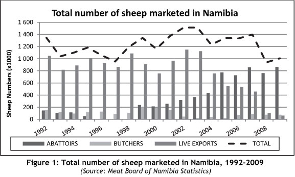
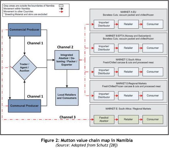
The value chain of Namibia's mutton production is shown diagrammatically in Figure 2. From this value chain map it is clear that there are various value chains, markets, and linkages between the various role players in the Namibian mutton industry. The on-farm production - as well as the marketing through various marketing channels to local and other various export markets - is depicted in Figure 2. The production figures of these channels are displayed in Figure 1.

 

 

As a result of the contribution of livestock production to the country's economy, research and planning in this sector are of paramount importance for a healthy, sustainable industry. This study will focus on the supply side of mutton production in Namibia with the aid of a supply response model that will be used to test the hypotheses of certain economic phenomena. Two hypotheses are tested in this study. The first is that climate factors play a major role in determining the supply response in the mutton industry. The second is that price-related factors also play a major role in determining the supply of mutton in the industry.

 

2. OVERVIEW OF SUPPLY RESPONSE STUDIES ON LIVESTOCK PRODUCTION

According to Huq & Arshad [7], supply response is a tool that is used to evaluate the effectiveness of price policies and to assist the producer in the allocation of resources. Supply response studies are also useful for evaluating production policies and incentives. The first studies on supply response were done in order to understand the price mechanism. Von Bach & Van Zyl [8] researched the supply response of beef in sixteen homogeneous and veterinarian areas in Namibia, using multiple regression techniques on biological and economic time series data. The approach to their study was based on the fundamentals of the work done by Nerlove [9]. However, Ogundeji, Jooste & Oyewumi [10] raised questions about Von Bach's results, due to possible multi-collinearity among the independent variables. Seleka [11] researched the short-run supply of small ruminants (including sheep and goats) in Botswana, using pooled data for six agricultural regions. Results obtained from this research showed that a 1% increase in sheep inventory results in a 1.23% rise in the number of sheep markets, where rainfall has no significant impact on sheep sales. The research also found that producer prices have no impact on small ruminant sales. However, for goat production, a 1% increase in rainfall leads to a 0.53% rise in goat marketing in the following year.

The most recent research was conducted by Ogundeji et al. [10] on the modelling of beef supply response in South Africa. With the aid of an error correction model (ECM), the supply response of beef production in South Africa was investigated. The independent variables in their supply model were rainfall; the real producers' price of beef, lamb, pork, chicken, and yellow maize; imports; and cattle populations that represented the climatic, economic, trade, and demographic factors. The production variables were modelled respectively to cattle marketed for slaughtering (dependent variable). Results showed that beef producers in South Africa respond to these production variables in the long-run. In the short-run, the results showed that the beef marketed is only responsive to climatic factors and the importing of beef. Results also showed that the supply model short-run adjustment speed of cattle marketed to the long-run equilibrium position is 63% of the proportion of disequilibrium. This means that 63% of disequilibrium from the long-run in cattle marketed is corrected within each year in the supply system.

 

3. SUPPLY RESPONSE APPROACHES

To measure agricultural output (supply responses to price and other non-price factors), two broad approaches can be followed: programming and econometrics [12].

3.1 Programming

Programming models, usually linear programming, involve the creation of a linear production model that represents the typical production system of a specific product or various products. An objective function is usually specified that is related to profit maximisation. Other objectives such as risk minimisation can also be defined.

By solving the model using various sets of data, and assuming that the profit is maximised, the supply-price relationship can be established for a specific product. The advantages of this approach are that linear programming is capable of handling complex multi- relationships at farm level in a production system. The complex multi-relationships involve recognition of all the effects of supply on product prices, input prices, and technological and physical restrictions. However, the data requirements are extensive: the collection of data at farm level is costly, and the development of such models takes a long time [13]. Due to the restricted data and resources that are available, this approach is not widely used by researchers when supply-response studies are conducted.

3.2 Econometric models

Production in agriculture is not instantaneous, and is dependent on post-investment decisions and expectations. From a practical perspective, the production in any period or season is affected by past decisions. The partial adjustment model used by Nerlove [9] is an early version of an econometric approach used to measure agricultural supply-response for a single commodity. Nerlove's partial adjustment model is used to capture agricultural supply response to price incentives. The general static supply function can be mathematically presented as:

where Y_t is the expected long-run equilibrium output level at time t; c is the constant term; β is the long-run supply response (rate of change); P_t_! is the output price at time t-1; γ is the coefficient of the linear deterministic time trend T; and fl_t is the independent normally distributed error term.

The dynamic adjustment of the supply response equation is based on Nerlove's hypothesis that "each year farmers revise the output level they expect to prevail in the coming year in proportion to the error they made in predicting the output level of this period". This is presented as:

where Y_t* is the expected output level at time t; and λ is the coefficient of expectation about price or elasticity if variables are expressed as logarithms. By substituting equation 1 in equation 2, we obtain:

where λβ captures the short-run price elasticity of supply.

According to Abou-Talb et al. [14] and Alemu, Oosthuizen & Van Schalkwyk [15], the Nerlovian partial adjustment model is considered weak for the following reasons. First, it displays an inability to distinguish between short-run and long-run elasticities. Second, the model uses integrated (non-stationary) series that pose the danger of spurious regression results. So it can be concluded that the partial adjustment model - used as a framework by many previous studies on supply response analysis - is less appropriate for the study of supply response on agricultural output due to its limitations, and due to the improvement in other methods.

Empirical dynamics of supply can also be described by error correction models (ECM). The ECM form of dynamic specification has been used by various authors in macro-economic modelling since its appearance in the Davidson, Hendry, Srba, & Yeo (DHSY) consumption function of 1978 [16]. The ECM offers a means of re-incorporating levels of variables alongside their differences, and hence of modelling long-run and short-run relationships between integrated series. In addition to this, economic time series data contain trends over time. Although regression analysis shows significant results with high R², the results may be spurious. ECM and co-integration analysis are used to overcome the problem of spurious regression [17].

The ECM approach is used to analyse non-stationary time series data that are known to be co-integrated. This method also assumes co-movement of the variables in the long-run. The general form of the ECM method is:

In this model, Δisa deference operator such that (ΔY_t =Y_t - Y_t_₁), where α defines the short-run supply elasticity, and β) the long-run supply elasticity. The Y_t's are assumed to be co-integrated time series variables (including other explanatory variables X_t__n).

Co-integration techniques received much attention because they solved the statistical problems associated with non-stationary data series leading to spurious regression results. Various co-integration approaches are available - all with some limitations and assumptions. The autoregressive distributed lag (ARDL) approach to co-integration, a relatively new approach to econometrics developed by Persaran, Shin & Smith [18], tests for the existence of non-spurious long-run relationships between economic variables. The ARDL model has the capacity (as mentioned earlier) to eliminate spurious regression results and to distinguish between long-run and short-run elasticities. Unlike other co-integration techniques for example Engle-Granger and Johansen, the ARDL model does not impose restrictive assumptions that all the variables in the study must be integrated to the same order. The effect of this is that the ARDL approach can be applied regardless of whether the underlying variables are stationary, non-stationary, or mutually integrated [19]. Another difficulty avoided by the ARDL approach concerns decisions about the number of endogenous and exogenous variables to be included, as well as the lags within these variables. The ARDL approach makes it possible to include in the supply model different variables that have a different optimal number of lags [20].

Due to these problems, researchers propose the direct estimation of the long-run parameters using unrestricted error correction models (UECM) that specify the inclusion of dynamics [21]. Due to the dynamic nature of production and market equilibrium, the dynamics arising from both dependent and independent variables need to be taken into account. Unrestricted dynamic models incorporating lagged and current values of both dependent and independent variables then become an autoregressive distributed lag model. The bounds-testing approach to the level relationship, together with the ADRL modelling approach to co-integration analysis developed by Persaran et al. [18], involves ordinary least square estimation of an ECM of the following:

In this expression, Δ is the first difference operator, α₀ is the constant, Y_t is the dependent variable, X_t is the independent variable, e_t is the error term, p and q are the maximum lag orders, is the long-run relationship (elasticities) among the variables, and β_i is the short- run relationship among the variables.The existence of a long-run level relationship in an ECM framework between the dependent variable Y_t and the independent variable X_t can be tested when it is not known whether the underlying independence is stationary, non- stationary, or mutually co-integrated with the ARDL approach.

The ARDL approach to co-integration analysis involves 2 stages.

The first stage involves the estimation of the ECM to compute the F-statistic (Wald test) that is used for testing joint significance of the coefficients of the lagged level independent variables (α₁,α₂,~α_ί) in the model. Here the joint significance is tested by testing the null hypothesis of no co-integration by setting all the lagged level variables equal to zero; or against the alternative hypothesis that the coefficients of all the lagged variables in the model are not equal to zero [22]. Considering the supply model in equation 5, the null hypothesis is:

Whether the F-statistic is significant is determined using critical values developed by Persaran et al. [18]. These are bounds containing a band of critical values with upper and lower limits for different significance levels. If the F-statistic lies above the upper bound for a specific significance level, a non-spurious long-run relationship exists among the variables in the ADRL model. If the F-statistic lies below the lower bound critical value, there is no long-run relationship among the variables in the ARDL model [23].

If the long-run relationship is confirmed with the Wald test among the variables, the second stage of the ARDL approach can be conducted. The second stage involves estimation of the long-run and short-run elasticities of the ADRL model. After the long-run relationship is confirmed among the variables, ordinary least square (OLS) regression is used to estimate the long-run and short-run elasticity coefficient of supply.

 

4. DATA AVAILABILITY AND SOURCES

The model used for this study - based on economic theory and previous work done in this field of the livestock industry - selects the variables influencing mutton supply. However, as mentioned earlier, it is not always possible to construct a model suggested by theory (because we cannot include all the variables initiated by theory due to the non-availability of data and quantification problems). The ideal would have been to include forward-looking factors of production in the supply model, in order to consider future risks in producers' decision-making regarding production. This was not taken into account due to quantification challenges. Therefore, the following unrestricted error correction type of ARDL model for mutton supply in Namibia was hypothesised in equation 7:

In this case, lnYt is the dependent variable of the mutton supply model, representing mutton marketed per month, and is measured in sheep (carcass) units. lnYt_n is a lag variable of mutton marketed, and is also included as an independent variable in the model resulting in a general autoregressive distributed lag model. lnNPt_n is the average monthly Namibian producer price, i.e. the average sheep slaughter price in N$/kg across the four export abattoirs in Namibia. lnPBt_n is the average monthly Namibian producer price for beef, i.e. the average beef slaughter price in N$/kg. The latter is included as an economic factor competing with mutton in the red meat market. lnRFt_n is the average monthly rainfall measured in millimeters per month across Namibia, and is included as a climatic factor influencing supply. a₇ for j=0 is the constant. a, for j=1 to 4 shows the long-run dynamics of the supply model. β3 for j=0 to 3 represents the short-run dynamics of the supply model. Δ is the first difference term, while et (error term) is the white noise disturbance term.

Theory rarely provides a basis for specifying the lag lengths in distributed lag models. In this ARDL model it is sensible to start at a maximum lag length of 12 months. This is the maximum lag length that is appropriate to the supply dynamics of sheep production in a production year.

According to Sarmiento et al. [24], previous studies lack tests for model performance to diagnose whether tests of the theory, or elasticity estimates, are subjected to different types of specification errors. Only a few studies on supply response go beyond the Durbin- Watson test in reporting the performance of their model specification. Emphasis is given to model specification tests to ensure that the hypothesised model is statistically significant. Specification tests include those for serial correlation, heteroscedasticity, model stability, a test for normality in the model residuals, and model specification (RESET test). A satisfactory result on the specification tests assures reliable results from the supply model, and is therefore an important part of the study.

The data required for the supply response analysis was obtained from the Meat Board of Namibia. Livestock marketed and livestock producer prices were obtained from monthly published reports. The rainfall was obtained from the Meteorological Service of Namibia. Data from three weather stations (Grootfontein, Windhoek, and Keetmanshoop) was used to calculate the country's monthly average that was used in the model. The Namibian price data was deflated to real price data by dividing the monthly nominal prices of the selected price variables by the monthly consumer price index (CPI) obtained from the Central Bureau of Statistics in Namibia. The response analysis time span covers the period January 2003 to December 2009.

 

5. RESULTS AND DISCUSSION

5.1 Time series properties of variables

The time series data of the selected variables first has to undergo analytical statistical tests before it can be used to compute short-run and long-run elasticities. The first test on the data is for seasonality. The most common approach is to use the method of dummy variables [25]. According to the goodness of fit, R², and the significance of the regression coefficients, sheep marketed [Y_t] and monthly rainfall [RF_t] are most likely to contain seasonal factors. The 'deseasonalisation' of the data by the dummy variable method is used to eliminate the seasonal component.

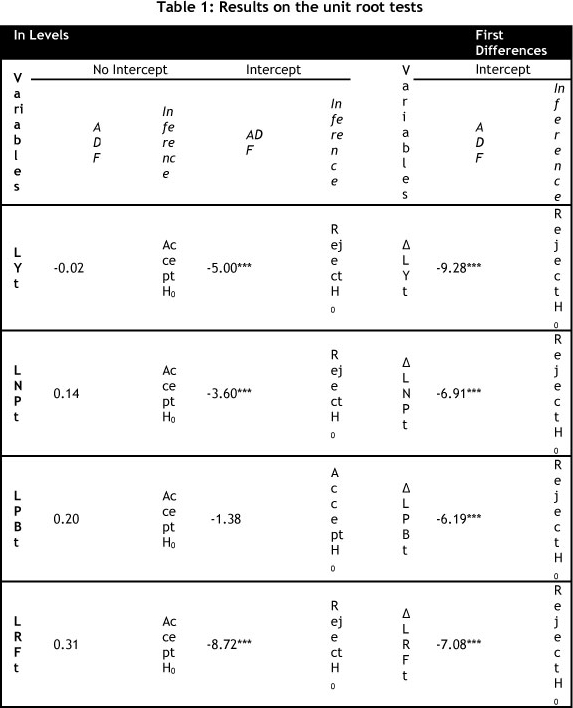
Stationarity properties of the supply model variables are determined. The ARDL approach followed in this study avoids the pre-testing requirement on the time series properties. However, the stationarity properties are needed to test for long-run relationship among the specified variables in the Engle-Granger and Johansen approach to co-integration. The Wald test incorporates the long-run relationship among variables, whether variables are non- stationary, stationary, or mutually co-integrated. The unit root test is therefore not applicable in the ARDL approach. However, it is still essential to complement the estimation process with a unit root test in order to be sure that the variables to be included in the analysis are not integrated to a higher order - i.e. I(2) [21].

From Table 1 we can conclude that none of the integrated variables in the mutton supply function are of an order higher than one With the stationarity properties of the data known, the next step of the supply response analysis, using the ARDL approach, can be conducted.

 

 

5.2 ARDL bounds test for co-integration

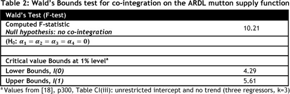
Once the ECM is specified and estimated, the next step is to test for the joint null hypothesis of no long-run level relationship. As mentioned in Section 3.2, the presence of a long-run relationship among the variables is tested with the aid of Wald's Bounds test². The results obtained from the Bounds test are presented in Table 2.

 

 

The stationarity properties of the data are used to retrieve the critical value bounds at 1% confidence level of Wald's Bounds test. Therefore it is important to determine the stationarity properties of the data.

The computed F-statistics for the mutton supply model in equation 7, based on Wald's test, are 10.21 (refer to Table 2). This result clearly exceeds the lower bound value I(0), of 4.29 at a 1% significance level. Thus the null hypothesis of no co-integration is rejected for the supply model, and a non-spurious long-run relationship is confirmed among the monthly mutton marketed, the real Namibian mutton producer price, the real Namibian beef producer price, and the monthly rainfall for mutton supply in Namibia. This result implies that these variables move together and so cannot move 'too far away' from each other independently [22]. From this result we can conclude that any disequilibrium among the variables in the supply model is a short-run phenomenon.

5.3 Model specification tests

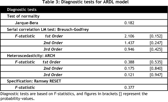
Misspecification in the regression is possible, making it is important to test the assumptions of the statistical model. According to Hendry & Nielsen [26], various tests are available to test misspecifications in regression models. These tests include those for normality, those for heteroscedasticity, and the regression specification error test (RESET) that was introduced by Ramsey in 1969 [26]. The validity of the specific mutton supply model is therefore confirmed by using the relevant diagnostic tests. (The tests included the Jarque- Bera test for normality, the Breusch-Godfrey test for serial correlation, the ARCH test for heteroscedasticity, the Ramsey RESET test for model specification, and the cumulative sum (CUSUM) and CUSUM of squares tests for model stability.

The Jarque-Bera statistic confirmed the normality behaviour of the residuals of the estimated mutton supply model (refer to Table 3). The Breusch-Godfrey LM test statistic rejects the first, second, and third order serial correlation in the mutton supply model. The ARCH tests verify that residuals are homoscedastic in the supply model. The Ramsey RESET test shows no evidence of functional form misspecification in rejecting the hypothesis of misspecification.

 

 

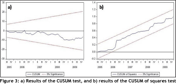
The CUSUM and CUSUM of squares tests validate the stability within the model parameters over the adjusted sample period of the mutton supply model. Figures 3 a) and b) show the CUSUM and CUSUM of squares tests for stability at a 5% significance level. According to Ogazi [20], the null hypothesis (i.e. that the regression equation is correctly specified) cannot be rejected if the plot of these CUSUM and CUSUM of squares statistics remain within the critical bounds of the 5% significance level. Thus, as the plots of the CUSUM and CUSUM of squares remain within the 5% significance bounds, it can be concluded that the statistics confirm the stability of the long-run coefficients in the model.

 

 

5.4 Long-run and short-run supply elasticities

The long-run elasticities of the production variables included in the mutton supply model, and which influence the supply, are calculated from the computed coefficients of the respective lag level independent variables (LNPt-1, LPBt-1, RFt-1), divided by the coefficient of the lag level dependent variable (LYt-1) of the specific ECM mutton supply model in Table 4. The results are given a negative sign to obtain the long-run supply elasticities of the different variables in mutton supply.

In explaining the long-run elasticities of equation 7, Table 5 shows the elasticities obtained from the analysis. All the long-run variables contain the expected signs and are statistically significant. The average real Namibian mutton price elasticity of supply is shown to be elastic by the expected positive sign. The practical implication is that if the average real Namibian mutton producer price increases by 1%, the mutton marketed will increase by 1.97% in the long-run. Related to this factor is the positive relationship between the mutton producer price and the number of sheep marketed. That is, the mutton producer's decision to market sheep for slaughter is positively influenced by price in the long-run. Similar long- run price elasticities of mutton supply were found in work done by Rezitis & Stavropoulos [27] on the Greek mutton industry. Rezitis et al. [27] found a long-run price elasticity of supply of 1.79 for the Greek sheep industry.

 

 

The average real Namibian beef producer price elasticity of supply is shown to be inelastic by a negative sign. In practical terms this is because when the beef price increases, mutton supply decreases in the long-run, due to the fact that mutton and beef are competing products. The reason for this behaviour is that producers start to reduce mutton production because beef production is more profitable as the beef price increases. The average real Namibian beef producer price elasticity of supply is -0.85. If the beef price increases by 1%, the mutton marketed will decrease by 0.85%.

The long-run price elasticity of competing products can be compared with those of Ogundeji et al. [10] who researched supply response of beef in South Africa. Their research obtained a competing product price elasticity of supply of -0.31. This is less than the results obtained in this study. The difference between these elasticities can be attributed to the fact that their work incorporated the price of various competing products (pork and beef) and not only one product (in this case, beef).

The long-run rainfall elasticity of supply is inelastic and has a positive sign. As expected, the positive sign of rainfall has a positive effect on mutton supply in the long-run. Therefore, as rainfall increases, mutton supply will increase. The long-run rainfall elasticity is 0.29, which means that when rainfall increases by 1% the mutton supply increases by 0.29% in the long- run. Long-run elasticity for rainfall obtained from Ogundeji et al. [10] is -0.25, compared with 0.29 in this study. The magnitude for these studies is the same; however the elasticities' signs are opposite. Ogundeji et al. [10] state that the negative influence of rainfall on supply appears when there is sufficient rainfall. The producers then tend to market less of their livestock in order to rebuild their stock that was depleted during the drought period. However, sufficient rainfall could also motivate producers to market their stock, as sufficient rain leads to good grazing conditions that accelerate stock-to-market readiness. The short-run elasticities are represented by the coefficients of the respective first differenced variables. When there is more than one coefficient for a particular variable in the short-run (coefficients of the differenced variables in equation 7), they are added, and their joint significance is tested using the Wald test.

Table 6 shows the short-run elasticities for the mutton supply function. The significance of the lagged coefficients was tested with the Wald test. Results on the short-run elasticities showed that the average real Namibian mutton producer price is elastic, and has a significantly negative effect on the mutton supply. This leads to the backward-bending supply curve. In practical terms it means that producers retain their livestock in response to price increases in the short-run, with the expectation of increased future income outweighing present income. The real Namibian beef producer price is inelastic, and has a positive effect on mutton supply in the short-run. This implies that producers market their current sheep stock in response to the beef producer price increase in the short-run, in order to expand their cattle stock as it becomes more profitable with the beef producer price increase.

 

 

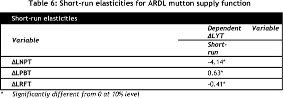
The rainfall short-run elasticity of supply is inelastic but negative. This result was also obtained by Ogundeji et al. [10]. The short-run negative effect indicates that good rainfall results in lower throughput (marketing of sheep) for slaughtering, probably due to the expectation that rainfall will result in better grazing conditions; and so producers hold back stock.

It is difficult to determine short-run elasticities due to the uncertainty in various factors influencing production. However, due to the significance of these short-run coefficients at a 10% confidence interval, these short run elasticities give good support to the long-run relationships. This implies the presence of significant short-run dynamics behind the long- run relationships [23]. The long-run elasticities have the opposite effect on mutton supply compared with the short-run elasticities. This behaviour can be attributed to the fact that producers' long-term and short-term production goals are different.

The error correction term (coefficient of LY_t-1) is statistically significant, and implies that there is adjustment back to the long-run (equilibrium) position once there is disturbance in the short-run due to shocks. The significance of the error term in the mutton supply function is another indicator of the presence of a long-run relationship among the variables included in the mutton supply model. The magnitude of the error correction term indicates the speed of adjustment back to the equilibrium position once the system is in disequilibrium. The error correction coefficient of -0.51 indicates that 51% of the previous month's deviation from long-run equilibrium is corrected in the current month. This means that a deviation from this month's equilibrium will take about two months to recover.

 

6. CONCLUSION

The ARDL approach to co-integration analysis was completed in two stages in order to generate the required relationships between dependent and independent variables within the supply model. The first stage involved the estimation of an unrestricted error correction model that included the dynamic nature of production. Through the elimination of insignificant variables from the model, a more specific error correction model was obtained. The second stage used the Wald test to confirm the existence of a long-run relationship among the variables in the supply model. Model specification tests were used to validate the model and the results obtained from the analysis. Therefore, with the aid of an appropriate approach, statistical software, and data, non-spurious results could be obtained for analysis of the mutton industry in Namibia.

Results showed that the producer price of mutton is a primary supply shifter for mutton supply in Namibia. An increase in the average Namibian producer price affects mutton supply positively in the long-run. Results also showed that the producer price of competing products (in this case, beef) has a negative effect on mutton supply in Namibia. Therefore it can be concluded that the hypothesis stating that price-related factors influence supply is accepted for this study. The supply response outcome showed that climate factors (rainfall) also have a significant effect on mutton produced in Namibia. An increase in rainfall has a positive influence on the amount of mutton produced. Thus the hypothesis stating that climate factors play a major role in mutton production in Namibia is also accepted for this study.

A supply response analysis of the mutton industry in Namibia illustrated the relevant importance of supply shifters towards production output. The decline in mutton production in Namibia since 2003 is a growing concern for industry stakeholders. The effect of the Scheme on total mutton production is debatable at this stage; however, production of mutton has shown a decline since the initiation of the Scheme. In future marketing policy- making, relationships between producer-price-related factors and production output can be used as a guideline for policy makers. The strong relationship between production output and producer price should make policy makers aware of the sensitivity of these factors to structural changes.

Forecasting for the mutton industry at this stage is important due to the declining trend in sheep marketed in recent years. Supply forecasts are useful, if not essential, for projecting current trends into future scenarios by producers, providers of infrastructure, downstream supply chain players, and policy makers. For supply chain players, forecasts are the foundation of informed decisions about future planning for capital expenditure (such as processing facilities). From a policy perspective, when investigating the status of mutton supply in Namibia, forecasts should be a forward-looking instrument to evaluate the small stock marketing scheme against its current intended goals. Considering that Namibia is a country where agriculture, especially livestock farming, is of primary importance, and where a high-value product is produced that is favoured by local and international markets, ongoing research in this field of study is required to secure a sustainable livelihood and economy for the people of Namibia. This study aims to contribute to the methodology as well as to the results it can obtain.

 

REFERENCES

[1] Ministry of Agriculture, Water and Forestry. 2009. Agricultural Statistics Bulletin (2000-2007). Directorate of Planning, Windhoek.         [ Links ]

[2] Motinga, D., Van Wyk, K., Vigne, P., Kauhika, S. & Visser, W. 2004. National small stock situation analysis. Windhoek, Namibia .         [ Links ]

[3] PWC. 2007. Evaluation of the implementation of the small stock marketing scheme in relation to the Namibian government's value addition goals and objectives. Windhoek.         [ Links ]

[4] Sweet, J. 1998. Livestock - Coping with drought: Namibia - A case study. Northern Regions Livestock Development Project. Tsumeb.         [ Links ]

[5] Von Bach, H.J.S. 1990. Supply response in the Namibian beef industry. MSc Thesis. Department of Agricultural Economics, University of Pretoria, Pretoria,         [ Links ]

[6] Kauika, S., Tutalife, C. & Montinga, D. 2006. Adding value with mutton: Is pricing everything? Institute for Public Policy Research, Briefing Paper No. 40.         [ Links ]

[7] Anwarul Huq, A.S.M. & Mohamed Arshad, F. 2010. Supply response of potato in Bangladesh: A vector error correction approach. Journal of Applied Sciences, 10(11), 895-902.         [ Links ]

[8] Von Bach, H.J.S. & Van Zyl, J. 1990. Supply of live cattle and of beef in Namibia. Agrekon, 29(4), 347-351.         [ Links ]

[9] Nerlove, M. 1958. Distributed lags and estimation of long-run supply and demand elasticities: Theoretical considerations. Agricultural & Applied Economics Association, 40(2), 301-311.         [ Links ]

[10] Ogundeji, A.A., Jooste, A. & Oyewumi, O.A. 2011. An error correction approach to modelling beef supply response in South Africa. Agrekon, Vol 50 (2), 44-58.         [ Links ]

[11] Seleka, T.B. 2001. Determinants of short-run supply of small ruminants in Botswana. Small Ruminant Research, 40, 203-214.         [ Links ]

[12] Colman, D. 1983. A review of the arts of supply response analysis. Review of Marketing and Agricultural Economics, 51(3), 201-230.         [ Links ]

[13] Thomson, K.J. & Buckwell, A.E. 1979. A microeconomic agricultural supply model. Journal of Agricultural Economics, 30(1), 1-11.         [ Links ]

[14] El-Wakil, A., Abou-Talb M., Mohy Al-din, M. & El Begawy, K.H. 2008. Supply response for some crops in Egypt: A vector error correction approach. Journal of Applied Sciences Research, 12(4), 1647-1657.         [ Links ]

[15] Alemu, Z.G., Oosthuizen, K. & Van Schalkwyk, H.D. 2003. Grain-supply response in Ethiopia: An error correction approach. Agrekon, 42(4), 389-404.         [ Links ]

[16] Hallam, D. & Zanoli, R. 1993. Error correction models and agricultural supply response. European Review of Agricultural Economics, 2, 151-166.         [ Links ]

[17] Tripathi, A. 2008. Estimation of agricultural supply response by cointegration approach. Research Report. Indira Gandhi Institute of Development Research, Mumbai.         [ Links ]

[18] Persaran, M.H., Shin, Y. & Smith, R.J. 2001. Bounds testing approaches to the analysis of level relationships. Journal of Applied Econometrics, 16, 289-326.         [ Links ]

[19] Odhiambo, N.M. 2009. Energy consumption and economic growth nexus in Tanzania: An ARDL bounds testing approach. Energy Policy, 37, 617-622.         [ Links ]

[20] Ogazi, C.G. 2009. Rice output supply response to the changes in real prices in Nigeria: An autoregressive distributed lag model approach. Journal of Sustainable Development in Africa, 11(4), 83-100.         [ Links ]

[21] Olokoyo, F.O., Osabuohien,E.S.C. & Salami, O.A. 2009. Econometric analysis of foreign reserves and some macroeconomic variables in Nigeria. African Development Review, 21(3), 454-475.         [ Links ]

[22] Hoque, M.M. & Yusop, Z. 2010. Impacts of trade liberalisation on aggregate import in Bangladesh: An ARDL bounds test approach. Journal of Asian Economics, 21, 37-52.         [ Links ]

[23] Getnet, K., Verbeke, W. & Viaene, J. 2005. Modeling spatial price transmission in the grain markets of Ethiopia with an application of ARDL approach to white teff. Agricultural Economics, 33, 491-502.         [ Links ]

[24] Sarmiento, C. & Allen, P.G. 1998. Dynamics of beef suply in the presence of cointegration: A new test of the backward-bending hypothesis. Review of Agricultural Economics, 22(2), 421-437.         [ Links ]

[25] Gujarati, D.N. 2006. Essentials of Econometrics. New York: McGraw Hill.         [ Links ]

[26] Hendry, D.F. & Nielsen, B. 2007. Econometric modeling - A likelihood approach. Princeton: Princeton University Press.         [ Links ]

[27] Rezitis, A.N. & Stavropoulos, K.S. 2009. Modeling sheep supply response under asymmetric price volatility and cap reforms. Economics Bulletin, 29(2), 512-522.         [ Links ]

[28] Schutz, W. 2009. A critical analysis of the Namibian value addition policy with reference to the small stock marketing scheme. Master of Business Administration. Department of Business Administration, Maastricht School of Management, The Netherlands.         [ Links ]

[29] Olubode-Awosola, O.O., Oyewumi, O.A. & Jooste, A. 2006. Vector error correction modelling of Nigerian agricultural supply response. Agrekon, 45(4), 421-436.         [ Links ]

[30] Lubbe, W.F. 1992. Price stabilisation policies: Has the meat scheme benefitted beef producers in South Africa? Agrekon, 31(2), 74-80.         [ Links ]

[31] Abbot, N. & Ahmed, A. 1999.The South African wool supply response. Agrekon, 38(1), 90-104.         [ Links ]

[32] Schutz, W. 2009. Report on the small stock marketing scheme. Meat Board of Namibia.         [ Links ]

 

 

* The author was enrolled for a master's degree in the Department of Industrial Engineering at Stellenbosch University.
1 Namibia imports 1.85% of its total mutton exports. This volume is mainly imported to the copper and diamond mines located near the South African border [28].
2 The stationarity properties of the data are used to retrieve the critical value bounds at 1% confidence level of Wald’s Bounds test. Therefore it is important to determine the stationarity properties of the data.