GENERAL ARTICLES

 

Analysing acceptance sampling plans by Markov chains

 

 

Mohammad Mirabi^{I, *}; Mohammad Saber Fallahnezhad^II

^IDepartment of Industrial Engineering Islamic Azad University, Ashkezar Branch, Iran M.Mirabi@yahoo.com
^IIDepartment of Industrial Engineering University of Yazd, Yazd, Iran Fallahnezhad@yazduni.ac.ir

 

 

---

ABSTRACT

In this research, a Markov analysis of acceptance sampling plans in a single stage and in two stages is proposed, based on the quality of the items inspected. In a stage of this policy, if the number of defective items in a sample of inspected items is more than the upper threshold, the batch is rejected. However, the batch is accepted if the number of defective items is less than the lower threshold. Nonetheless, when the number of defective items falls between the upper and lower thresholds, the decision-making process continues to inspect the items and collect further samples. The primary objective is to determine the optimal values of the upper and lower thresholds using a Markov process to minimise the total cost associated with a batch acceptance policy. A solution method is presented, along with a numerical demonstration of the application of the proposed methodology.

---

OPSOMMING

In hierdie navorsing word 'n Markov-ontleding gedoen van aannamemonsternemingsplanne wat plaasvind in 'n enkele stap of in twee stappe na gelang van die kwaliteit van die items wat geïnspekteer word. Indien die eerste monster toon dat die aantal defektiewe items 'n boonste grens oorskry, word die lot afgekeur. Indien die eerste monster toon dat die aantal defektiewe items minder is as 'n onderste grens, word die lot aanvaar. Indien die eerste monster toon dat die aantal defektiewe items in die gebied tussen die boonste en onderste grense lê, word die besluitnemingsproses voortgesit en verdere monsters word geneem. Die primêre doel is om die optimale waardes van die booonste en onderste grense te bepaal deur gebruik te maak van 'n Markov-proses sodat die totale koste verbonde aan die proses geminimiseer kan word. 'n Oplossing word daarna voorgehou tesame met 'n numeriese voorbeeld van die toepassing van die voorgestelde oplossing.

---

 

 

1. INTRODUCTION

Acceptance sampling designs are methods used for decision-making about incoming batches. They include a sample size and a decision rule. The sample size is the number of items to be inspected, while the decision rule works out how to use the inspection result to accept or reject the lot. Acceptance sampling plans also involve quality contracting on items between vendor and buyer. Such sampling plans provide vendor and buyer with rules for lot sentencing to satisfy their pre-set requirements on product quality. Various designs for methods of acceptance sampling that improve the quality of items have been presented by many researchers. Klassen [1] proposed an acceptance sampling system based on a new measure named 'credit', in which the credit of the producer is defined as the total number of items accepted since the last rejection. Tagaras [2] considered a Markovian deteriorating machine, and proposed a new process control and machine maintenance policy. Kuo [3] developed an adaptive control policy for machine maintenance and product quality control. Ferrell & Chhoker [4] proposed an acceptance sampling design based on the Taguchi loss function by considering deviations between a quality characteristic and its target level. Pearn & Wu [5, 6] introduced a variable sampling plan based on one-sided process capability indices. Niaki & Fallahnezhad [7] used a Bayesian inference concept to design an optimal sampling plan. They formulated the problem as a stochastic dynamic programming model to minimise the ratio of total discounted system cost to a discounted system correct choice probability. Moskowitz & Tang [8] proposed acceptance sampling plans based on the Taguchi loss function and a Bayesian approach. Ferrell & Chhoker [9] developed mathematical models that can be used to design both 100% inspection and single sampling plans. McWilliams et al. [10] provided a method of finding exact designs for single sample acceptance sampling plans. Aslam et al. [11] presented acceptance sampling plans for a generalised exponential distribution when the lifetime experiment is truncated at a predetermined time. Aminzadeh [12] proposed acceptance sampling plans based on the assumption that successive observations on a quality characteristic are auto-correlated. Aminzadeh [13] also derived Bayesian economic acceptance sampling plans using the Inverse Gaussian model and a step-loss function.

In this research, a Markov chain for acceptance sampling plans in both single and two stages of a decision-making process is proposed, in which the optimal policy is derived on the basis of the quality of items inspected. The number of defective items in each stage is compared with the optimal upper and lower thresholds, and decision-making is modelled by a Markov process. Thereafter the rest of the paper is organised as follows. The problem is first stated in Section Two. The notations are presented in Section Three. Next, the single-stage model, together with an illustrative example, is proposed in Section Four. Section Five contains the two-stage model along with a numerical example. The paper is concluded in Section Six.

 

2. PROBLEM STATEMENT AND ASSUMPTIONS

Consider a batch that contains a specific item. At each stage of the batch acceptance policy, the states of the batch are defined in terms of the quality of the items inspected. This quality is determined by using attribute acceptance sampling plans to accept or reject a production lot. The accept/reject decision is based on the count of the number of defective items [5]. If this number is greater than an upper threshold, the batch should be rejected. If it is less than a lower threshold, the batch should be rejected. If it is between the upper and lower thresholds, the process of sampling and inspecting continues. The objective is to find the optimal values of the thresholds that minimise the total cost associated with the batch acceptance strategy

 

3. NOTATIONS

To model the problem, the following notations are used:

E(AC): The expected total system cost

E(AC): The expected total cost of accepting the batch

E(RP): The expected total cost of rejecting the batch

E (I): The expected total cost of inspecting the batch

n : The sample size of a single-stage batch acceptance strategy

n₁: The sample size in the first stage of a two-stage batch acceptance strategy

n₂: The sample size in the second stage of a two-stage batch acceptance strategy

N : The number of total items in a batch

p : The proportion of defective items in a batch

c₁: The lower threshold for the number of defective items in the first stage

c2 : The upper threshold for the number of defective items in the first stage

c₃: The lower threshold for the number of defective items in the second stage

c₄: The upper threshold for the number of defective items in the second stage

I : The cost of inspecting an item in the batch

c : The cost of producing a defective item

R : The cost of batch rejection

δ₁: The minimum acceptable level of the lot quality (acceptable quality level (AQL)).

δ₂: The minimum rejectable level of the lot quality (lot tolerance proportion defective) (LTPD))

ε>₁: The probability of type-one error in making a decision

ε₂ : The probability of type-two error in making a decision

P: The transition probability matrix

Q: The square matrix containing the transition probabilities of going from a non-absorbing state to another non-absorbing state

R: The matrix containing all probabilities of going from a non-absorbing state to an absorbing state (i.e., finished or scrapped product)

A: An identity matrix representing the probability of remaining in a state

O: The matrix representing the probabilities of escaping an absorbing state (always zero)

M: The fundamental matrix containing the expected number of transitions from any non-absorbing state to another non-absorbing state before absorption occurs

F: The absorption probability matrix containing the long-run probabilities of the transition from any non-absorbing state to an absorbing state

pij.: The probability of going from state i to state j in a single stage

m_ij: The expected number of transitions from a non-absorbing state (i) to another non-absorbing state (j) before absorption occurs

f_ij: The long-run probability of going from a non-absorbing state (i) to an absorbing state (j)

 

4. MODEL DEVELOPMENT

Consider a batch acceptance policy where decision-making is based on the number of defective items. A sample of the proper size is first gathered for inspection, based on the number of decision-making stages (either one stage or two). Then the decision about accepting, rejecting, or carrying out more inspection is made. The purpose of this research is to develop a Markovian model to determine the optimum values of the thresholds for each inspection stage. The paper first develops the model for a single stage, and then proposes the two-stage acceptance policy.

Based on the notations defined in Section Three, the expected total system cost can be expressed as follows:

In what follows, the optimal batch acceptance policy is first derived. Then the modelling extends to the two-stage case in Section 5.

4.1 A single-stage acceptance sampling policy

Assume a single-stage sampling policy that is defined as follows: n items will be inspected. If the number of defective items is below a lower control threshold c₁, then the batch will be accepted. If the number of defective items is above a control threshold c₂ then the batch is rejected; and if the number of defective items falls between the thresholds c₁ and c₂, the process of inspecting n more items continues. If p denotes the proportion of the defective items in the batch, we have:

Probability of inspecting n more samples=

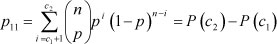
Probability of accepting the batch=

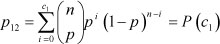
Probability of rejecting the batch=

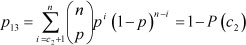
Where P (c) denotes the cumulative distribution function of binomial distribution with parameters (n, p). The states of the problem are defined as follows:

State 1: n more items should be inspected.

State 2: the batch should be accepted.

State 3: the batch should be rejected.

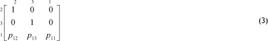
The transition probability matrix among the states of the batch can be expressed as follows:

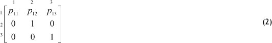
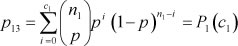
Where p₁₁ is the probability of inspecting n more items, p₁₂ is the probability of the batch being accepted, and p₁₃ is the probability of the batch being rejected.

The matrix P is an absorbing Markov chain where states 2 and 3 are absorbing states and state 1 is a transient state. Analysing this absorbing Markov chain requires a rearrangement of the transition matrix in the following form:

The fundamental matrix M can be obtained as follows:

where m₁₁ represents the expected number of times in the long run that the transient state 1 is occupied before absorption occurs (i.e., accepted or rejected), given that the initial state is 1 and I is the identity matrix. The long run absorption probability matrix, F, can be calculated as follows:

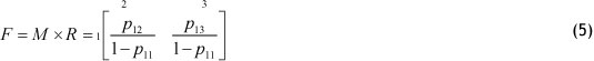
The elements of the F matrix, f₁₂ f₁₃, represent the probabilities of the batch being accepted and rejected respectively. The expected total system cost given in Equation (1) can now be derived. The expected acceptance cost, E(AC), is determined by the expected cost of the defective items c(Np) multiplied by the absorption probability of a batch being accepted (i.e., f₁₂). The expected rejection cost, E(RP), is obtained by the rejection cost, R, multiplied by the absorption probability of the batch being rejected (i.e., f₁₃). The expected inspection cost is also given by Inm₁₁. Therefore the expected cost for the batch acceptance policy can be expressed as a function of f₁₂ f₁₃,, and m₁₁ as follows:

Substituting for f₁₂ and m₁₁ , the expected cost equation can be rewritten as:

In terms of the cumulative binomial distribution, equation (7) becomes:

where the terms P (c₁) and P (c₂) are functions of the probability of producing a defective item p.

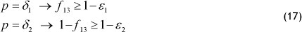
The optimal acceptance policy becomes a matter of determining the values of c₁ and c₂, which minimise the expected total system cost numerically. Alternatively, in order to determine the boundary limits of c₁ and c₂, the concept of type-I and type-II error probabilities is utilised. The type-I error, ε₁, shows the probability of rejecting the batch when the defective percentage of the batch is acceptable; and the type-II error, ε₂, is the probability of accepting the batch when the percentage defective is not acceptable. Then, if p = δ₁, the probability of rejecting the batch is less than ε₁; and if p = δ₂, the probability of accepting the batch will be less than ε₂. Hence we have:

Based on the above inequalities, the feasible values of c₁ and c₂ among a set of alternative values are first determined. The optimal acceptance policy is then derived using Equation (9). A numerical example is given in the next subsection to illustrate the application of the proposed methodology.

4.2 An illustrative example

To demonstrate the application of the proposed methodology in a batch single-stage acceptance strategy, a numerical example is solved in this section. Consider a single-stage system with the number of items in a batch N = 1000, the proportion of the defective items in a batch is p = 0.1, the cost of a defective item c = 6, the cost of batch rejection R = 600 , the cost of item inspection I = 3 , the number of items in an inspected lot n = 50 , δ1 = 0.05, δ2 = 0.2, ε₁= 0.05, and ε₂= 0.1.

The feasible values of c₁ and c₂ among existing alternatives are first obtained using Equation (9) as follows:

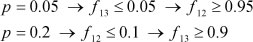
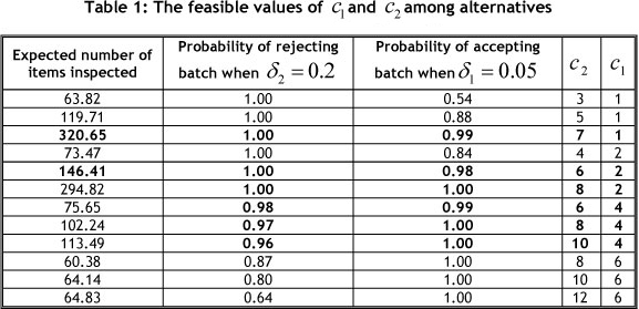
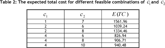
In other words, the probability of accepting the batch when δ1 = 0.05 should be greater than 0.95, and the probability of rejecting the batch when δ2 = 02 should be greater than 0.9. Table 1 shows 12 different alternative combination values of c₁and c2 together with their probability of rejecting or accepting the batch, of which the ones in bold are feasible. Equation (8) is then numerically solved for all feasible sets of Table 1. The results are given in Table (2). Based on the results, the best combination value is c1 = 4 and c2 = 6 with the minimum value for the expected total cost of 826.94.

 

 

 

 

5. A TWO-STAGE BATCH ACCEPTANCE POLICY

In a two-stage batch acceptance strategy, assume that a lot containing n_i items is first inspected. If the number of defective items in the lot is less than or equal to c₁, then the batch is in a good state and is accepted. If the number of defective items is more than c₂, the batch is rejected. Otherwise, if the number of defective items is greater than c₁, but less than or equal to c₂ , a sample of n₂ items is inspected and the batch is evaluated in the second stage. In the second stage, a lot containing an additional n₂ items is inspected.

If the total number of defective items is less than or equal to c₃ , the batch is accepted. If the total number of defective items is greater than c₃, but less than or equal to c₄, a lot containing an additional n₁ items is inspected and then the two-stage decision-making process starts over. Otherwise, if the total number of defective items is more than c₄, the batch is rejected.

As in the single-stage acceptance strategy, a Markov chain process with the following states can model the above decision making:

State 1: The first stage acceptance policy should be applied to the batch

State 2: The second stage acceptance policy should be applied to the batch

State 3: The batch should be accepted

State 4: The batch should be rejected

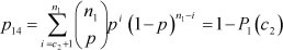
Then, based on the notations given in Section Three, the first stage probability of accepting the batch is

The first stage probability of rejecting the batch is

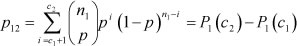
The first stage probability of deciding in the second stage is

The second stage probability of accepting the batch is

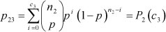
The second stage probability of deciding in the first stage is

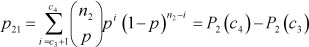
The second stage probability of rejecting the batch is

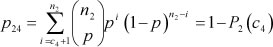
where P₁ (.) and P₂ (.) denote the cumulative binomial distribution functions of stage 1 and stage 2 of the decision-making process.

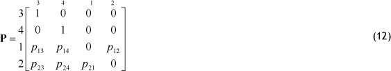
In this case, the transition probability matrix P can be expressed as follows:

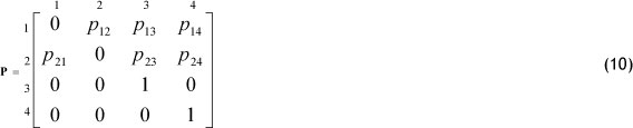
Again, to analyse this absorbing Markov chain, the single-step probability matrix should be rearranged in the following form:

Rearranging the P matrix in the latter form yields the following matrix:

The fundamental matrix M can be obtained as follows [14]:

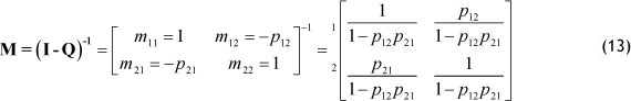
where m_ii represents the expected number of times in the long run that the transient state i, (i = 1,2) is occupied before absorption occurs (i.e., accepted or rejected), given that the initial state is 1.

The long run absorption probability matrix F can then be calculated as follows [14]:

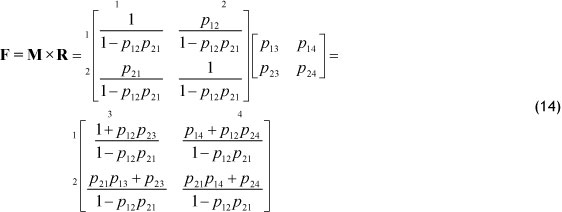
where f₁₄ is the probability of rejecting the batch.

The expected total system cost can now be obtained using Equation (1). The expected acceptance cost is simply the acceptance cost (cNp) multiplied by the probability of accepting the batch at stage 1 (i.e. f₁₃). The expected rejection cost is the rejection cost ( R ) multiplied by the probability of rejecting the batch at stage 2 (f₁₄). The expected inspection cost is the inspection cost ( I ) multiplied by the number of batch inspections at stage 1 (i.e., m11 ) multiplied by the number of items inspected (n1) plus inspection cost ( I ) multiplied by the number of batch inspections at stage 2 (i.e., m22 ) multiplied by the number of items inspected, (n₂), multiplied by the probability of continuing to the second stage (p₁₂) . Therefore the expected cost for a two-stage acceptance sampling policy can be expressed as follows:

Or

Then, similar to what was derived in a single stage, one obtains:

In the next subsection, a numerical example is given to illustrate the application of the proposed methodology.

5.1 An illustrative example

Consider a two-stage system with the number of items in a batch N = 1000, the proportion of the defective items in a batch p = 0.1, the cost of a defective item c = 6, the cost of batch rejection R = 600 , the cost of item inspection I = 3 , the first sample size in an inspected lot n1 = 50 , the second sample size n2 = 40, δ₁ = 0.05, δ2 = 0.2, ε1 = 0.05, and ε2 = 0.1.

The feasible values of c1,c2,c3, and c₄ are obtained among existing alternatives, using Equation (17).

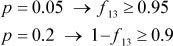
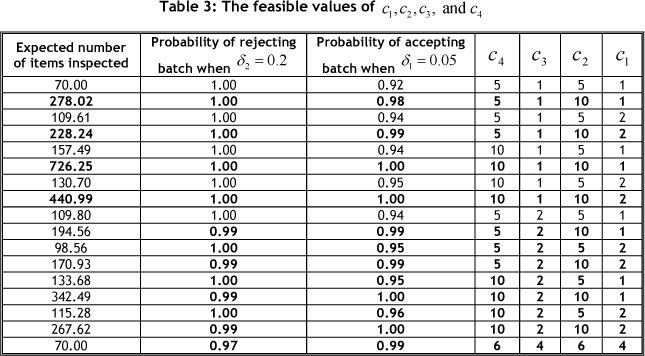
In other words, the probability of accepting the batch when δ1 = 0.05 should be greater than 0.95, and the probability of rejecting the batch when δ2 = 0.2 should be greater than 0.9. Table 3 shows 16 different alternative combination values of c1,c2,c3, and c₄together with their probability of rejecting or accepting the batch, of which the ones in bold are feasible.

Subsequently, Equation (16) is numerically solved for all feasible sets of Table 3. The results are given in Table 4. Based on the results, the best combination value is c₁ = 4 and c₂ = 6, c₃ = 4 and c₄ = 6 with an objective function value of 810.

 

 

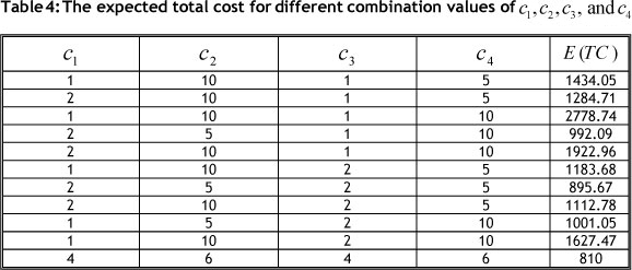
Comparing the performance of the two sampling procedures, it can be seen that the minimum value cost for a single sampling plan occurs when c₁ = 4 and c₂ = 6 , where the probability of first error type is 0.01, the probability of second error type is 0.02, the expected number of inspected items is 75.65, and the total expected cost is 826.94. The minimum cost of a two stage sampling plan occurs in c₁ = 4 and c₂ = 6 , c₃ = 4 and c₄ = 6

where the probability of first error type is 0.01, the probability of second error type is 0.03, the expected number of inspected items is 70, and the total expected cost is 810. It is therefore concluded that a two-stage sampling plan has marginally better performance.

 

6. CONCLUSION

This paper deals with the optimum value of control thresholds in an acceptance sampling design determined numerically by using a Markovian approach. The paper initially develops a general model for the expected cost by considering acceptance, rejection, and inspection costs. The model is subsequently used to determine the optimum value of control thresholds for a single-stage and a two-stage acceptance strategy. Numerical examples are solved to demonstrate the application of the proposed methodology. The results of the numerical example show that a two-stage acceptance strategy has marginally better performance.

 

REFERENCES

[1] Klassen, C.A.J. 2001. Credit in acceptance sampling on attributes. Technometrics, 43, 212-222.         [ Links ]

[2] Tagaras, G. 1998. Integrated cost model for the joint optimization of process control and maintenance. Journal of Operational Research Society, 39, 757-766.         [ Links ]

[3] Kuo, Y. 2006. Optimal adaptive control policy for joint machine maintenance and product quality control. European Journal of Operational Research, 171, 586-597.         [ Links ]

[4] Ferrell W.G. & Chhoker, J.A. 2002. Design of economically optimal acceptance sampling plans with inspection error. Computers & Operations Research, 29, 1283-1300.         [ Links ]

[5] Pearn, W.L. & Wu, C.W. 2006. Critical acceptance values and sample sizes of a variables sampling plan for very low fraction of defective. Omega, 34, 90-101.         [ Links ]

[6] Pearn, W.L. & Wu, C.W. 2007. An effective decision making method for product acceptance, Omega, 35, 12-21.         [ Links ]

[7] Niaki, S.T.A. & Fallahnezhad, M.S. 2009, Designing an optimum acceptance plan using Bayesian inference and stochastic dynamic programming. International Journal of Science and Technology (Scientia Iranica), 16(1), 19-25.         [ Links ]

[8] Moskowitz H. & Tang, K. 1992. Bayesian variables acceptance-sampling plans: Quadratic loss function and step loss function. Technometrics, 34(3), 340-347.         [ Links ]

[9] Ferrell, W.G. & Chhoker, A. 2002, Design of economically optimal acceptance sampling plans with inspection error. Computers & Operations Research 29, 1283-1300.         [ Links ]

[10] McWilliams, T.P., Saniga, E.M. & Davis, D.J. 2001. On the design of single sample acceptance sampling plans. Economic Quality Control, 16(2), 193-198.         [ Links ]

[11] Aslam, M., Kundub, D. & Ahmada, M. 2010. Time truncated acceptance sampling plans for generalized exponential distribution. Journal of Applied Statistics 37(4), 555-556.         [ Links ]

[12] Aminzadeh, M.S. 2009. Sequential and non-sequential acceptance sampling plans for autocorrelated processes using ARMA(p,q)models. Comput Stat 24, 95-111.         [ Links ]

[13] Aminzadeh, M.S. 2003. Bayesian economic acceptance sampling plans using Inverse-Gaussian model and Step-Loss function. Commun Stat Theory Methods 32, 961-982.         [ Links ]

[14] Bowling, S.R., Khasawneh, M.T., Kaewkuekool, S. & Cho, B.R. 2004. A Markovian approach to determining optimum process target levels for a multi-stage serial production system. European Journal of Operational Research 159, 636-650.         [ Links ]

 

 

* Corresponding author