


Serviços Personalizados
Artigo
 Inglês (pdf)
 Artigo em XML
 Referências do artigo
Indicadores

Links relacionados
-
 Citado por Google
 -
 Similares em Google
Compartilhar

 Permalink
South African Journal of Economic and Management Sciences
versão On-line ISSN 2222-3436
versão impressa ISSN 1015-8812
S. Afr. j. econ. manag. sci. vol.21 no.1 Pretoria 2018
http://dx.doi.org/10.4102/sajems.v21i1.2001
ORIGINAL RESEARCH
Factor structure of South African financial stocks
Sudhir Madaree
Financial Services Institute of Australasia (FINSIA), Australia
ABSTRACT
BACKGROUND: The financial sector within the locally listed equity market is an important component of the economy. Understanding the inherent risks of this sector is vital from a portfolio risk management perspective, as such insights can aid in protecting against capital loss in the event of exposure to risk factors in this sector.
AIM: The study aims to identify and explain the principal risk factors over time inherent to the financial stock sector of the locally listed equity market, accompanied by explaining the volatility of such principal risk factors.
SETTING: The study looks at financial sector stocks within the South African listed equity space from June 2007 to March 2017.
METHODS: The methods used to perform such an investigation were twofold, namely, factor analysis to statistically identify risk factors latent in a basket of financial sector firms and generalised autoregressive conditional heteroscedasticity (GARCH) analysis to examine the volatility of the principal risk factors.
RESULTS: The findings suggest that the heterogeneity of risk factors within the financial sector has burgeoned in the past five years, explaining a large proportion of risk during this period. However, over the long-term, banks appeared to have been the main factor driving risk within the financial sector, explaining around 55% of risk. The volatility of banks was most noticeable during business cycle falls that were underpinned by known economic or political instability.
CONCLUSION: Banks have been the riskiest factor within financial sector firms over the past decade, explaining more than 50% of risk in recent years and notably susceptible to economic and political uncertainty.
Introduction
The financial sector represents an important part of the economy, as it facilitates the savings and investment process of economic agents. Understanding the risks inherent in such a sector is vital, particularly from a portfolio risk management perspective. Insight into the risks can aid in protecting against capital loss in the event of large exposure to such risk factors.
The past several years have borne witness to economic and political events that have caused a steady decline in the credit ratings of local banks and sovereign bonds. The most recent downgrade by S&P of foreign-denominated South African debt to junk status is an outcome of the challenging effects of local economic and political conditions (South African Reserve Bank [SARB] 2017). These uncertainties have the ability, ceteris paribus, to impact the profitability of firms within the financial sector, particularly banks (Appleton 2016). Amid a sluggish growth environment, this trend reinforces lower profitability.
A related aspect of deteriorating sentiment concerns the impact of capital flows on the stock prices of listed firms, such as those of banks, and the consequent volatility associated with these price movements. Portfolios may utilise listed equity markets such as the Johannesburg Stock Exchange (JSE) All Share Index in portfolio construction, which the financial sector is inherently a component of. From a portfolio risk management perspective, it is important to identify risk factors latent within a sector and explain the volatility over time. This may allow one to protect against capital loss, particularly portfolios that are substantially exposed to financial sector stocks.
Several studies in the literature have discussed the behaviour of listed stocks from international and local perspectives. From a local perspective, Moolman and du Toit (2005) examined the relationships between the South African stock market and macroeconomic variables from Q3 1987 to Q4 2000 using an error correction technique. This was intended to capture the short-term dynamics between the variables in question. Results revealed that in the short-term, volatilities or fluctuations in the local stock market were caused by macroeconomic variables, such as, inter alia, short term interest rates, the Rand/US$ exchange rate and the gold price.
Szczygielski and Chipeta (2015) utilised an asset-pricing model, namely, the arbitrage pricing theory (APT) to explain the risk factors of South African stocks from July 1995 to March 2011. Results revealed that various factors explained the behaviour of the South African stock market, namely, local inflation, changes in money supply, oil prices, real economic activity and the Rand/US$ exchange rate.
Van Rensburg (1995) utilised a multifactor model to examine the relationship between the local stock market and several macroeconomic factors, namely, term structure of the interest rate, returns of the New York Stock Exchange, the gold price and inflation expectations. Results revealed all four factors were significant drivers of local stock prices.
From an international perspective, Mouna and Anis (2016) investigated the sensitivity of returns in three financial sectors to macroeconomic variables, namely, the interest rate, stock market and the exchange rate using an adapted generalised autoregressive conditional heteroscedasticity (GARCH) model during the financial crisis. Eight countries were sampled and examined during this time period (2006-2009). Results revealed that overall across the eight countries, stock market returns, exchange rate volatility and interest rates had significant effects on the returns of the three financial sectors (banks, financials and insurance) during the financial crisis.
Zeng et al. (2014) examined whether the United States of America (US) banks played an important role in explaining the volatility of US stocks. The authors utilised a multifactor model based on monthly returns of US stock portfolios, size and value factors from January 1980 to December 2007. Results revealed that the banking risk factor significantly explained volatility in stock returns.
Schuermann and Stiroh (2006) examined the common factors that drove US bank stock returns from 1997 to 2005 using several multifactor models. Results revealed that the market factor noticeably drove the returns in bank stocks, with interest-related factors not being helpful in explaining such return behaviour of banks, particularly for the largest banks.
Berkowitz (2001) utilised the Fama and French (1993) model for determining common risk factor drivers of Canadian stock returns. The author used this type of multifactor model on monthly Canadian stock returns from January 1982 to December 1999. It was revealed that three factors explained the major part of the volatility in Canadian stocks over time.
The above studies in conjunction with a scan of available literature suggested no apparent presence of studies, at least locally, that have examined inherent risk factors within particular sectors of listed equities through time, such as the financial sector. Thus, a knowledge gap exists, which this study aims to fill by offering scientific value to the local literature. To investigate the problems of identifying and explaining the intertemporal principal financial sector risk factors and their related volatilities, two statistical models were employed. Firstly, factor analysis was used to extract risk factors latent within local financial sector stocks over three-year, five-year and 10-year periods. The aim was to identify the main risk factors and any changes in those factors. Secondly, because time-series variables tend to exhibit volatility clustering properties, a GARCH (1,1) model was used to explain the volatility of identified principal risk factors through time. This allowed us to clearly identify periods in which principal risk factors were volatile, and to attach economic rationale to those periods of volatility. The methodology and data section is followed by the Results section. The final section provides the concluding remarks.
Methodology and data
Data
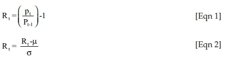
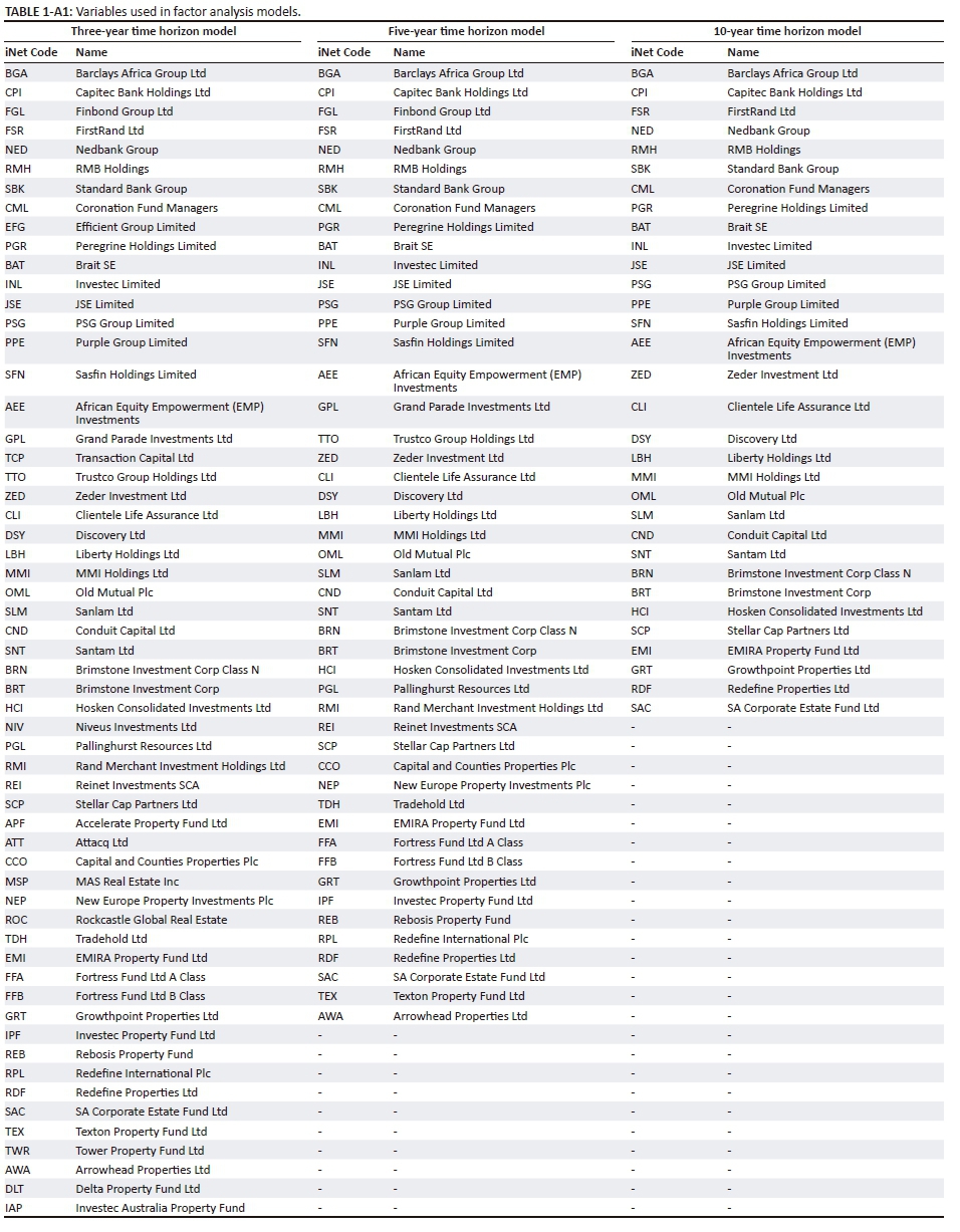
Data for all financial sector stocks listed on the JSE main board between June 2007 and May 2017 were obtained from the data provider iNet BFA, denominated in South African Rands (ZAR). This was the method used to obtain the financial sector stocks. The financial sector comprises stocks from the industry membership groups of banks, insurance, real estate and financial services (FTSE Russell 2016). Weekly pricing history was utilised for all variables and was converted into monthly returns (Equation 1) and standardised (Equation 2) for factor extraction. Details on the variables appear in Appendix 1.
Factor analysis was conducted to extract risk factors latent within local financial sector stocks over three-year (short-term), five-year (medium term) and 10-year (long-term) time horizons. The respective monthly data points were 156, 260 and 520. Prior to standardisation, variables were checked for consistency regarding weekly returns. Those that did not have such on a frequent basis were excluded from the analysis. Thus, the sample size diminished as the time horizon increased, representing a limitation to this study.
All variables used in the study were standardised or normalised through the calculation of Z-scores, which has the effect of preserving the normality nature of the variables in question, particularly transforming variables into new scores with a mean of zero and a unit standard deviation (Abdi & Williams 2010). A Z-score for each observation of a variable is calculated by subtracting the mean of the variable from each observation's value, and then dividing the answer by the standard deviation of the variable in question (refer to Eqn 2). Mean centring and autoscaling are critical in factor analysis as they allow all variables to have equal importance in contributing to the analysis.
Factor analysis
Factor analysis extracts uncorrelated factors latent in a data set, with the approach aiming to explain most of the variance for the data, particularly the covariance between underlying variables. Factors constitute linear combinations of underlying variables, typically from a transformed matrix based on standardised variables such as a correlation coefficient matrix (Landau & Everitt 2004). Standardisation is critical as it centres the mean of each variable to allow for comparative analysis.
Factors are analogous to eigenvectors, with each eigenvector exhibiting an eigenvalue. An eigenvalue represents a measure of variance in all variables within a data set. Various factor extraction methods can be used, such as principal components analysis (PCA), principal factor analysis (PFA) and the maximum likelihood method (Iacobucci 2001). The PFA method was employed for this study as an appropriate method to extract the factors, as it takes into account uniqueness or measurement error of the underlying variables (Landau & Everitt 2004). In other words, PFA extracts factors based on the degree of variation between variables, whereas PCA extracts factors based on the level of variance within individual variables. The higher the level of common variance (known as communality) and the lower the level of uniqueness (non-common variation) of a variable, the more relevant the variable becomes in explaining the meaning of a factor.
Fundamentally, eigenvalues of a square matrix were computed using Equation 3:

where:
-
A = i*i matrix
-
v = column vector of eigenvectors
-
λ = eigenvalue or determinant
Equation 3 above is analogous to an optimisation or maximisation problem solved by the Lagrange-Multiplier λ. The PFA method uses spectral decomposition as suggested by Anderson-Rubin in 1956 (StataCorp 2013) to segment a correlation coefficient matrix into factors, assuming i variables and j factors:
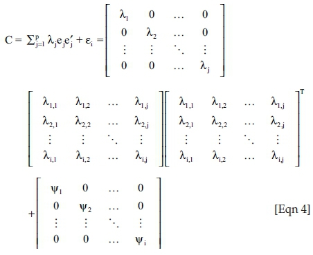
where:
-
C = i*i correlation coefficient matrix
-
λj = j*j diagonal eigenvalue matrix
-
ej = i*j factor loading matrix orthogonal in nature
-
 = transpose of ej
 -
εi = i*i diagonal matrix of residuals/uniqueness
After factor extraction is complete, rotation of the factors is required to clarify the interpretation of the factors (Yong & Pearce 2013). Traditionally, orthogonal varimax rotation is used as it preserves the lack of correlation among factors (Walker & Maddan 2013). This rotation approach geometrically rotates the extracted factors to form 'new' (adjusted) axes in a clockwise manner, causing the factors to remain perpendicular or orthogonal to each other. Mathematically, rotated loadings of underlying variables become correlated close to one in one eigenvector and close to 0 in other eigenvectors. Ideally, each factor should have a few large positive loadings and a large number of small or negative loadings.
After factor rotation, the last step is to describe the extracted factors, and to interpret their meaning in terms of economic theory. The factor analysis method is underpinned by variables that exhibit high loadings and low uniqueness levels clustering together (Yong & Pearce 2013); the researcher then attaches a description based on these clustered variables. Common descriptions refer to the fundamental characteristics of stocks, such as valuation metrics and industry memberships. Valuation metrics entail using valuation measures of stocks, such as price-to-book and earnings growth levels, to describe variables. Industry membership entails using the nature of the business based on revenue generation to describe the variables. The latter method was used in this study.
The generalised autoregressive conditional heteroscedasticity model
Generalised autoregressive conditional heteroscedasticity models are a type of conditional volatility model. The GARCH model explains and forecasts the volatility of time-series variables that exhibit autocorrelation and heteroscedasticity. A GARCH (1,1) model assumes that the best predictor of the current period's error variance is a function of a weighted long-run variance average, information obtained in the previous period (squared residual) and the previous period's variance (Poon & Granger 2005). Equation 5 is as follows:

In essence, GARCH transforms each original variance at time t to be conditional upon the above three terms, thus taking into account heteroscedasticity and autocorrelation. This method provides a robust way to explain volatility through time (Engle, 2001). Although other models exist that are able to explain through time volatility of financial variables, such models were not investigated as this was not the sole focus of the paper. Thus, a robust, parsimonious and popular model was selected to show through time volatility of financial variables that exhibited heteroscedasticity and autocorrelation, namely, the GARCH (1,1) model. The statistical software Stata was used to run factor analysis and GARCH analysis in this study.
Results
Factor extraction
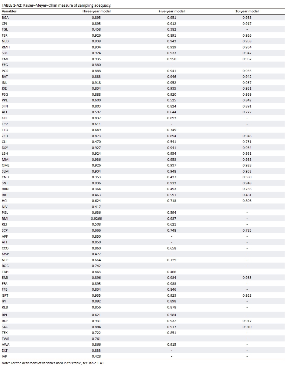
A prerequisite for factor extraction is that variables must show moderate to moderately high levels of correlation. This enables factors to be extracted and underlying variables to be assigned to the factors. The data conformed to this requirement, as confirmed by the high Kaiser-Meyer-Olkin (KMO) values of 0.865 for the short-term, 0.908 for the medium-term and 0.9336 for the long-term models, respectively (details provided in Appendix 2). The KMO statistic measures the proportion of variance among variables that might be shared. As a general rule, a KMO value of between 0.8 and 1 indicates sampling adequacy.
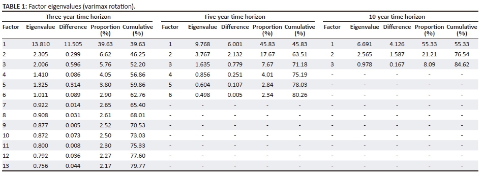
Table 1 shows the rotated factors that account for approximately 80% of the variance - hence volatility - in the financial sector. In this particular case, the variance can be labelled as risk in the financial sector. Over the short, medium and long terms, a single factor (Factor 1) stands out as explaining a large proportion of risk. The variance of this factor has diminished in recent years; it explained only 39% of variance (risk) over the most recent three-year period, compared with 55% over the longer 10-year period. However, Factor 1 still accounts for a large proportion of financial sector risk.
The sample size across the three time horizons was not consistent, owing to certain stocks not having a complete pricing history. This implies that the stock composition of the financial sector appears to have expanded during recent years. The sample was smallest for the 10-year time horizon and largest for the three-year time horizon (these details are provided in Appendix 1). This difference might explain the dilution in volatility contributed by Factor 1 for the shorter time horizons. The risk composition of the financial sector appears to have become more diverse, with a greater number of risk factors witnessed over the short-term that explain approximately 80% of the financial sector risk.
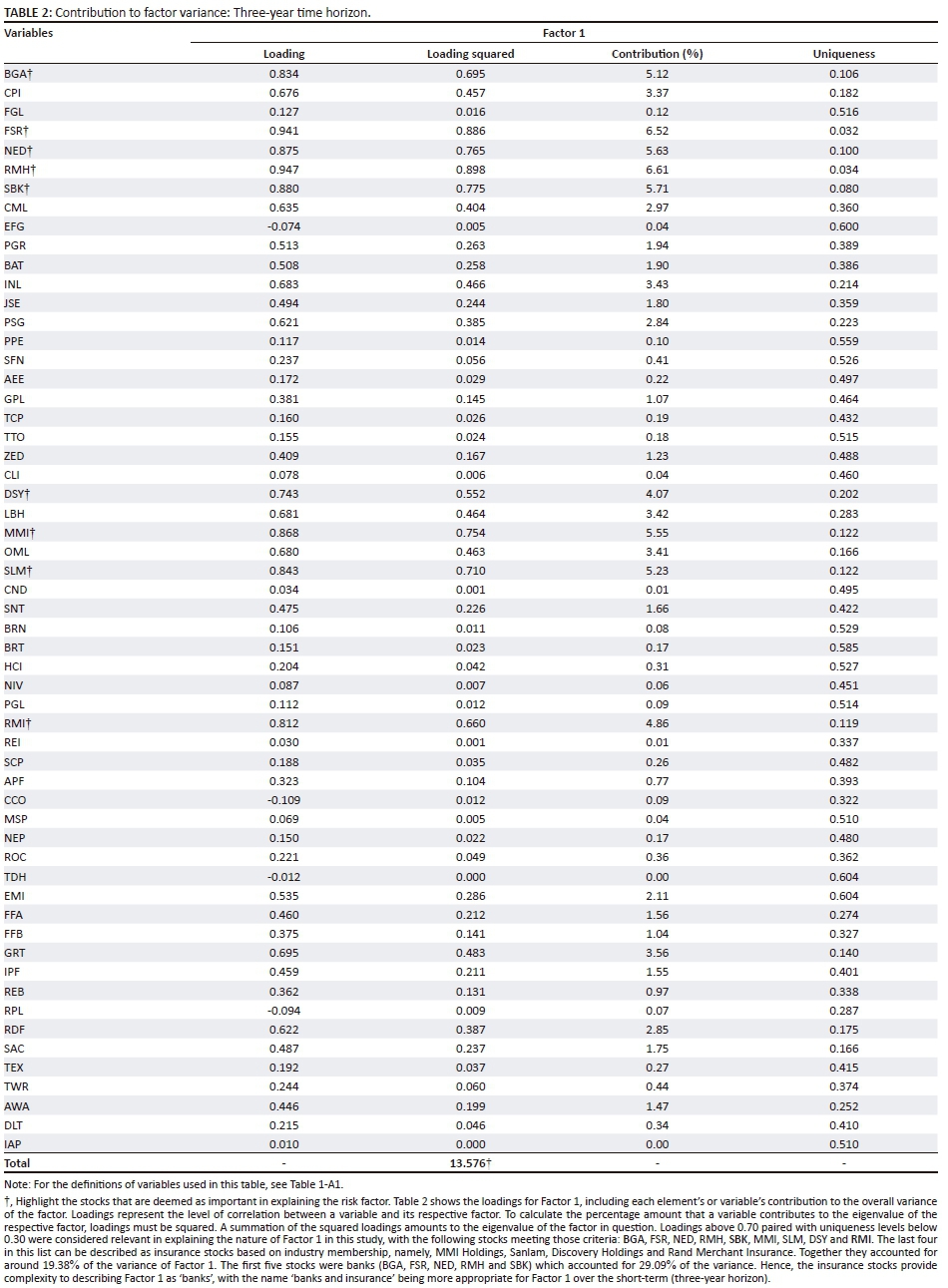
With the proliferation of short term risk factors latent in the financial sector and the dilution of risk emanating from Factor 1 over the short-term, the question arises: what does Factor 1 comprise? Answering this question would allow economic meaning to be attached to the factor. An inherent problem within factor analysis is the subjectivity in naming or describing factors. An approach to quantitatively naming the factors is to refer to the level of variance a variable contributes to the overall eigenvalue of the factor, in conjunction with the level of uniqueness of the variable in question. Highly unique variables imply a lesser relevance in explaining the factor in question. Table 2 shows the loadings for each model and the variance each variable contributed to Factor 1. As Factor 1 accounts for a large amount of volatility across the three time horizons, it is the focus of this paper.
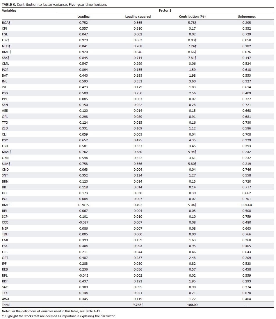
Table 3 shows a similar level of loadings over the medium term, with most of the same stocks appearing to have the greatest relevance in explaining the variance of Factor 1. However, bank stocks appear to have greater relevance than insurance stocks, accounting for around 37.82% of the variance in Factor 1, compared with the 16.78% accounted for by MMI, SLM and RMI. (DSY accounted for less than 4.5% and was therefore dropped from explaining the factor.) None of the insurance stocks had loadings in excess of 0.8, unlike in the short term model. Thus, for the five-year time horizon, Factor 1 can best be described more clearly as 'banks'.
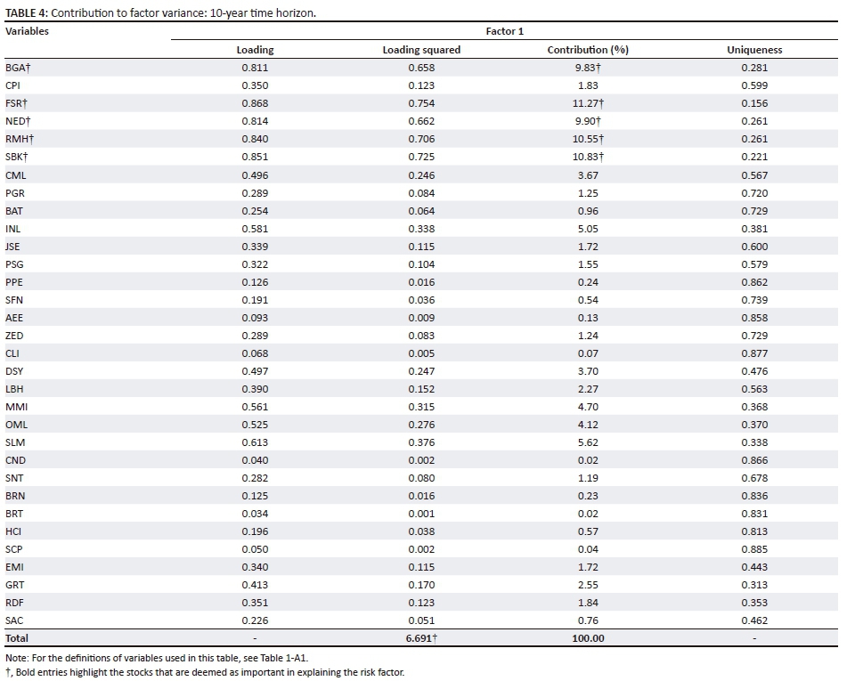
Table 4 shows loadings over the long-term, with bank stocks clearly appearing to account for most of the variance of Factor 1 at around 52.38%. None of the insurance stocks had high enough loadings and low enough uniqueness levels to attach much importance to their role in describing Factor 1. Thus, for the 10-year horizon, banks contributed most to the risk in the financial sector and it is reasonable to describe Factor 1 as 'banks'. This finding provides impetus for examining the volatility of banks more in detail as it is the principal risk factor. The 'GARCH Analysis section' of this paper provides an explanation of the use of a GARCH (1,1) model to investigate the FTSE/JSE South African Banks Total Return Index. The GARCH (1,1) was selected as it represents a simple version of the GARCH model and provides parsimony to the analysis.
The generalised autoregressive conditional heteroscedasticity analysis
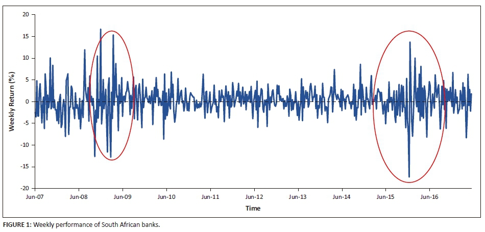
Figure 1 shows the weekly performance of South African banks over the past decade, proxied by the FTSE/JSE SA Banks Total Return Index. The data were obtained from iNet BFA. Graphically, there have been periods where volatility has clustered, highlighted by the red circles. This pattern renders the data appropriate for a GARCH model, which requires data to exhibit volatility clustering so that the model can appropriately explain volatility through time. A prerequisite for using GARCH is to determine whether an autoregressive conditional heteroscedasticity (ARCH) effect exists; the Lagrange-Multiplier (LM) test is used for this purpose (Abonongo, Oduro & Ackora-Prah 2016). The LM merely tests whether coefficients in a regression are jointly equal to zero, implying no ARCH effect. This null hypothesis must be rejected to statistically confirm that ARCH effects do exist. The output from the LM test on our data can be found in Table 5.
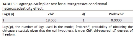
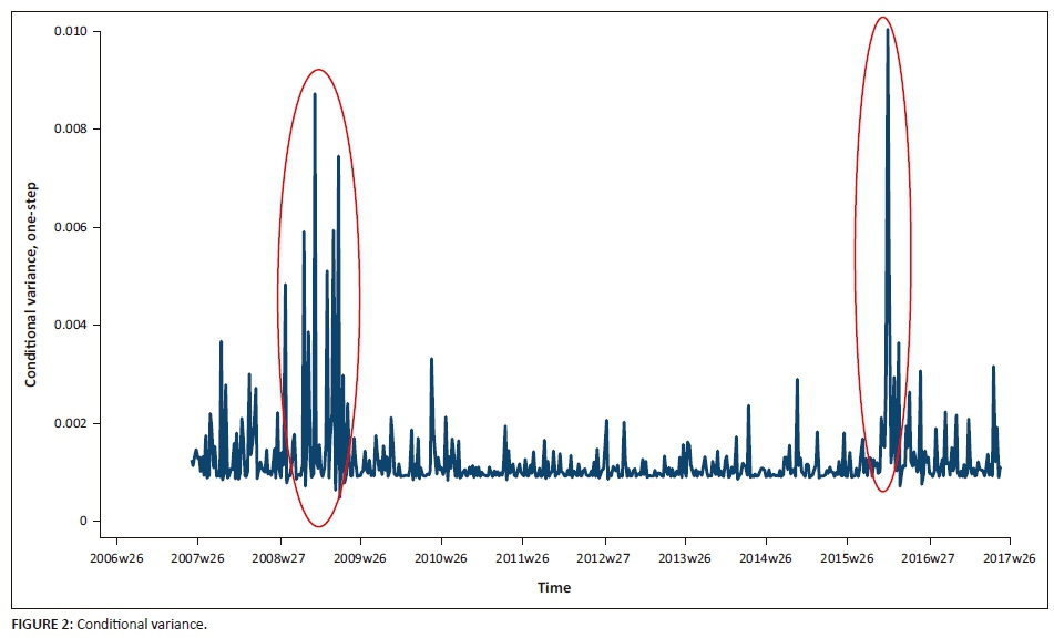
Table 5 shows a p-value less than 0.0001, which is highly significant. This means the null hypothesis ('there is no ARCH effect') can safely be rejected and the need for a GARCH model to explain the volatility is required. We, therefore, ran the GARCH (1,1) model on the data for weekly returns in the SA Bank Index. The start point was Week 22 of 2007 (03 June 2007) and the end point was Week 20 of 2017 (14 May 2017). The output of the GARCH (1,1) model transformed the original residuals as a function of Equation 5. A visual depiction of these transformed values is shown in Figure 2, which highlights various periods in which volatility has clustered.
Of particular interest are the clusters highlighted in red circles in Figure 2. The first circle approximately represents the period October 2008 to March 2009, and the second circle approximately represents the period December 2015 to January 2016. The first period coincided with a fall in South Africa's business cycle, a period of volatility and uncertainty. This decline in the business cycle can be attributed to the global financial crisis (GFC). Figure 3 shows an estimation of the business cycle using the Hodrick-Prescott (HP) filter method to decompose seasonally adjusted real gross domestic product (GDP) into its trend component and cyclical component. The latter represents the business cycle (Hodrick & Prescott 1997). Seasonally adjusted real GDP data were obtained from the South African Reserve Bank (SARB). The HP filter minimises the following function to determine the trend within seasonally adjusted real GDP:
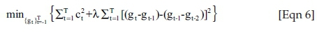
The first term of Equation 6 above represents the sum of the squared deviations of output at time t from the trend. The second term represents the sum of squared second differences in the trend penalised by the Lagrange (λ) parameter (Hodrick & Prescott 1997). The λ parameter represents the extent to which the trend is required to be made smooth. Such a parameter is required to be specified, with a rule of thumb for calculating the estimation - that is, λ = 100*(number of periods in a year)2. Quarterly data, for example, are given the parameter of 1600. Thus, the cyclical component is calculated by the difference between actual output and its trend.
The second period also coincided with a decline in the business cycle, witnessed from the start of 2015, a period rife with political instability. A case in point was the dismissal of Finance Minister Nene early in December 2015, which resulted in a sharp increase in the yield of the South African sovereign 10-year note by over 10%. This raised government borrowing costs and impacted bank stocks. Although no causality can be inferred from this apparent association, the pattern clearly shows that bank stocks are extremely volatile during periods of economic and political uncertainty, ceteris paribus.
Conclusion
The heterogeneity of risk factors inherent within the financial sector has burgeoned in recent times, explaining a large proportion of the risk within the sector. This trend appears to be because of the expansion of stocks within the financial sector. However, over the long-term (10-year horizon), a single risk factor evidently drove most of the risk (55%), and three risk factors collectively explained around 84% of the risk in the financial sector over the same period. Using industry membership as a basis to describe principal risk factors, it was clear that banks represented the principal risk factor over the long-term. Banks have been significantly volatile over two periods within this long-term time horizon, as shown by the GARCH analysis. The first period coincided with the fall in South Africa's business cycle, precipitated by the GFC. The second period was because of increased political risk (ceteris paribus) immediately after the dismissal of Finance Minister Nene, suggesting that economic and political risks have an intense effect on banks. The increased heterogeneity of risk factors within financial stocks in the short-term (three-year horizon) holds implications for portfolio risk management. Portfolios having wide exposure to the financial sector require one to be cognisant of the increased array of risk factors now present. Such awareness may aid in protecting against capital loss in the event of increased economic and political uncertainty. Given the current landscape in South Africa, such a scenario seems fairly probable at present.
Acknowledgements
The findings and interpretations of the paper are solely those of the author and should not be attributed to FINSIA.
Competing interests
The author declares that he has no financial or personal relationships that may have inappropriately influenced him in writing this article.
Authors' contributions
The author declares that he has no financial or personal relationships that may have inappropriately influenced him in writing this article.
References
Abdi, H. & Williams, L., 2010, 'Normalizing data', in N. Salkind, D. Dougherty & B. Frey (eds.), Encyclopedia of research design, pp. 935-938, Sage, Thousand Oaks, CA. [ Links ]
Abonongo, J., Oduro, F. & Ackora-Prah, J., 2016, 'Modelling volatility and the risk-return relationship of some stocks on the Ghana Stock Exchange', American Journal of Economics 6(6), 281-299. [ Links ]
Appleton, M., 2016, Know your asset attributes, Global Perspectives, Ashburton Investments, Bellville, South Africa, p. 19. [ Links ]
Berkowitz, M., 2001, Common risk factors in explaining Canadian equity returns, Working papers, University of Toronto, Department of Economics Toronto. [ Links ]
Engle, R., 2001, 'GARCH 101: The use of ARCH/GARCH models in applied econometrics', Journal of Economic Perspectives 15(4), 157-168. https://doi.org/10.1257/jep.15.4.157 [ Links ]
Fama, E. & French, K., 1993, 'Common risk factors in the returns on stocks and bonds', Journal of Financial Economics 33, 3-56. https://doi.org/10.1016/0304-405X(93)90023-5 [ Links ]
FTSE Russell, 2016, Industry classification benchmark (equity), viewed 06 June 2017, from http://www.ftse.com/products/downloads/icb_rules.pdf [ Links ]
Hodrick, R. & Prescott, E., 1997, 'U.S. business cycles: An empirical investigation', Journal of Money, Credit and Banking 29(1), 1-16. https://doi.org/10.2307/2953682 [ Links ]
Iacobucci, D., 2001, Journal of consumer psychology's special issue on methodological and statistical concerns of the experimental behavioral researcher, Lawrence Erlbaum Associates, Mahwah, New Jersey. [ Links ]
Landau, S. & Everitt, B., 2004, A handbook of statistical analyses using SPSS, Chapman & Hall/CRC Press, Boca Raton, FL. [ Links ]
Moolman, E. & du Toit, C., 2005, 'An econometric model of the South African Stock Market', SAJEMS 8(1), 77-91. [ Links ]
Mouna, A. & Anis, J., 2016, 'Market, interest rate, and exchange rate risk effects of financial stock returns during the financial crisis: AGARCH-M approach', Cogent Economics & Finance 4(1), 1-16. https://doi.org/10.1080/23322039.2015.1125332 [ Links ]
Poon, S. & Granger, C., 2005, 'Practical issues in forecasting volatility', Financial Analyst Journal 61(1), 45-56. https://doi.org/10.2469/faj.v61.n1.2683 [ Links ]
South African Reserve Bank (SARB), 2017, Financial stability review first edition 2017, Financial Stability Department, Pretoria. [ Links ]
Schuermann, T. & Stiroh, K., 2006, Visible and hidden risk factors for banks, FRB of New York Staff Report No. 252, Econstor, FRB of New York, New York. [ Links ]
StataCorp LP., 2013, Stata multivariate statistics reference manual, Stata Press, College Station, TX. [ Links ]
Szczygielski, J. & Chipeta, C., 2015, 'Risk factors in returns of the South African stock market', Journal for Studies in Economics and Econometrics 39(1), 47-70. [ Links ]
Van Rensburg, P., 1995, 'Economic forces and the Johannesburg stock Exchange: A multifactor approach', De Ratione 9(2), 45-63. https://doi.org/10.1080/10108270.1995.11435059 [ Links ]
Walker, J. & Maddan, S., 2013, Statistics in criminology and criminal justice, Jones & Barlett Learning, Burlington, NJ. [ Links ]
Yong, A. & Pearce, S., 2013. 'A beginner's guide to factor analysis: Focusing on exploratory factor analysis', Tutorials in Quantitative Methods for Psychology 9(2), 79-94. https://doi.org/10.20982/tqmp.09.2.p079 [ Links ]
Zeng, L., Yong, H., Treepongkaruna, H. & Faff, R., 2014, 'Is there a banking risk premium in the US Stock Market', Journal of Financial Management, Markets and Institutions 2(1), 27-42. https://doi.org/10.12831/77235 [ Links ]
 Correspondence:
Sudhir Madaree
sudhirmadaree@yahoo.co.uk
Received: 28 June 2017
Accepted: 20 July 2018
Published: 11 Sept. 2018
Table 1 - A1 - Click To Enlarge

