ORIGINAL RESEARCH

 

An investigation into the ability of the reverse yield gap to forecast inflation and economic growth in South Africa

 

 

Keren A. Gossman^I; Mark G. Hayes^II

^ISchool of Statistics and Actuarial Science, Faculty of Science, University of the Witwatersrand, South Africa
^IIDepartment of Mathematics and Statistics, Faculty of Science and Engineering, Curtin University, Australia

Correspondence

 

 

---

ABSTRACT

BACKGROUND: Monetary policy in South Africa is carried out by the South African Reserve Bank (SARB) with the aim of keeping inflation within a target range of 3% - 6%. The SARB uses a variety of models to aid them, with the core model being the most significant.
AIM: The primary aim of this research is to determine whether the reverse yield gap (RYG) contains information that could be useful to the SARB when making monetary policy decisions.
SETTING: The authors found no evidence that similar studies on the RYG have previously been done in the South African context. Since the yield curve has been found to be significant in South Africa at forecasting economic growth, yet insignificant in Europe, the results for this research may too be different to the global experience.
METHODS: The authors tested for linear relationships between the RYG and economic growth and inflation over the period 1960-2014.
RESULTS: The results indicate that a slight linear relationship may exist in the case of economic growth, with the RYG based on earnings yields showing better out-of-sample forecasting abilities. Further investigation indicates that the linear relationship is stronger during times of economic upturn. The results for inflation forecasting, however, show no signs of a reasonable linear relationship.
CONCLUSION: There is evidence for the SARB to consider whether the RYG can replace other economic variables in its core model without loss of predictive ability. Interestingly, this study found evidence to suggest that the RYG has an inverse relationship to future economic growth in South Africa, which is not what was expected.

---

 

 

Introduction

The reverse yield gap (RYG) is generally given to be the difference between the gross redemption yield on long-term government bonds and the dividend yield (Armah & Swanson 2011; Davis & Fagan 1997) or the earnings yield on domestic equities (Maio 2013).

Research on the usefulness of the RYG in predicting economic conditions such as future economic growth and inflation (Armah & Swanson 2011; Davis & Fagan 1997) as well as stock market returns (Maio 2013) has been done in the United Kingdom (UK) as well as the United States (US). Nobili (2006) explains that if the prices of assets in the market are set by rational investors then it must be that yield spreads, such as the RYG, contain information about investors' expectations for the future.

Armah and Swanson (2011) investigate the use of a carefully chosen set of economic variables in predicting economic growth and inflation to assist with monetary policy decisions in the US. Yield spreads, such as the RYG, are ideal variables for such models as they are simple to determine and can often be obtained before the values of other macro-economic variables are available (Davis & Fagan 1997; Nobili 2006). This adds further interest to the idea of exploring the forecasting abilities of the RYG if the results found can be useful to the South African Reserve Bank (SARB) in monetary policy decision-making.

The primary aim of this study was to determine if the RYG contains information that could be useful to the SARB when making monetary policy decisions. The focus of the research was not how the RYG could be used by the SARB, but rather to take the initial step of investigating how well the RYG can forecast economic conditions in South Africa.

The authors expect to accomplish this primary aim by achieving two subaims, the first being to investigate the ability of the RYG to forecast inflation levels in South Africa. The second is to determine the ability of the RYG to forecast economic, gross domestic product (GDP) growth in South Africa. Under this aim the relationship between the RYG and economic growth will be investigated over the full data set used in the study and then over periods that are classified as economic upwards phases and economic downwards phases.

This article has the following structure. The 'economic implications of the reverse yield gap' section describes the economic implication of the RYG; the 'past research' section is a literature review; 'the data' section gives a description of the data and variables; the 'history of the reverse yield gap' section reviews the history of the RYG; the 'in-sample linear modelling' section describes the in-sample linear modelling; the 'out-of-sample forecasting' section covers the out-of-sample forecasting models; the 'forecasting gross domestic product over different economic periods' section investigates forecasting economic growth during upwards and downwards business cycles; the 'conclusions' section details the authors' conclusions.

 

Economic implications of the reverse yield gap

Prices of financial assets

The notion that a yield spread contains information on future market conditions is driven by the idea that asset prices are set by rational investors based on their expectations of the future (Nobili 2006). Hence, current financial yield spreads contain useful information about future economic conditions (Davis & Fagan 1997).

Equity prices give an indication of the market's expectations of future profitability, which should be affiliated to future economic growth (Davis & Fagan 1997). Conventional bond prices should be more affected by future inflationary expectations, since equities are generally real assets which inherently provide investors with inflation protection. Thus, the RYG can be expected to provide information on future inflationary expectations to the extent that these expectations affect the relative prices of conventional bonds and equities (Davis & Fagan 1997).

The efficient market hypothesis

One should note that the ideas presented in the 'prices of financial assets' section rely on the assumptions that, first, investors have access to all relevant information influencing future economic conditions and, second, that investors are rational and can accurately formulate expectations and price for them (Timmermann & Granger 2004). One needs to then consider the efficiency of the market concerned.

A semi-strong form efficient market is one where all publicly available information is contained in asset prices, while a strong form efficient market is one where all public and privately available information is contained in asset prices (Fama 1970; Finnerty 1976). Thus, the amount of information contained in asset prices, which are priced as suggested in the 'prices of financial assets' section, will depend on the degree of efficiency in the South African market. A strong form efficient market would be ideal; however, asset prices in a semi-strong form market may still provide sufficient information on future economic and market conditions.

Investigating the level of efficiency of the South African market is beyond the scope of this article; however, it is worth noting that if the RYG is not predictive it may be a result of inefficiency in the market or that investors are not rational.

Monetary policy in South Africa

Monetary policy in South Africa is carried out by the SARB with the aim of keeping the rate of increase in the consumer price index (CPI) within a target range of 3% - 6%.¹

The use of various models is central to the process of monetary policy decision-making, with the core model being the most significant of these models (Aron & Muellbauer 2007; Smal, Pretorius & Ehlers 2007). The SARB began developing the core model in 1974 to model the South African economy (Smal, Pretorius & Ehlers 2007). The model is a quantitative, macro-economic model and comprises a number of stochastic equations for important factors (Smal, Pretorius & Ehlers 2007). Since its initial development, the model continues to undergo continual reviews and modifications (Smal, Pretorius & Ehlers 2007).

The core model is used to quantify the impact on the South African economy of different monetary policy decisions, with the main components of the model aimed at explaining inflation, GDP and the exchange rate (Smal, Pretorius & Ehlers 2007).

Smal, Pretorius and Ehlers (2007) explain that while a successful model should incorporate large amounts of information there is still a desire for relative simplicity. The RYG would be a useful addition for forecasting inflation and GDP due to its simplicity and the ease with which financial spreads can be observed (Davis & Fagan 1997; Nobili 2006). Smal, Pretorius and Ehlers (2007) make no mention of the RYG already being included as a factor in the core model as at December 2006.

It is unlikely that the RYG alone can provide sufficient forecasting ability; however, it may contain some marginal forecasting ability. Thus, it may well be found that replacing a number of factors currently contained in the core model with the RYG could result in no significant loss of forecasting ability while at the same time reducing the number of variables and increasing the ease and simplicity of using the model.

 

Past research

Europe

Davis and Fagan (1997) developed univariate models for European countries to predict inflation and economic growth. Their initial models were autoregressive models using past data for inflation and economic growth to predict values. The RYG was then added to each model and they were tested for any improvements. Their results show little evidence that the RYG could be used effectively as an indicator for future economic growth and inflation in European countries; however, the results for economic growth were slightly better than those for inflation.

Modelling techniques that allow for time variation of coefficients were used by Nobili (2006) in an attempt to determine if this could improve the marginal predictive strength of the RYG. Nobili measured the significance of the RYG by first constructing a benchmark model to forecast GDP and inflation in the Euro area. His benchmark model was a Bayesian vector autoregressive model with time-varying coefficients and economic explanatory variables. He found that the addition of the RYG as a predictor in the model made slight, statistically insignificant, improvements.

The general consensus is that the RYG has poor out-of-sample performance in forecasting economic growth and inflation and that the estimated parameters are unstable over time (Davis & Fagan 1997; Nobili 2006).

Duarte, Venetis and Paya (2005) found that when using some other financial spreads to forecast economic growth, a non-linear model yielded better results than their linear model and had more success at forecasting economic growth during periods of slow growth.

Investigating the use of non-linear models is, however, beyond the scope of this article.

The United States

Armah and Swanson (2011) aimed to show that a carefully chosen set of macro-economic variables can contain the same relevant information as a larger and more complex financial data set. The authors measured this relevance in terms of being useful for monetary policy decisions and forecasting economic conditions, in particular inflation and economic growth. Armah and Swanson (2011) found that the addition of the RYG, as well as some other financial spreads, did not improve the forecasting ability of their models.

South Africa

The authors found no previous research on the usefulness of the RYG in predicting inflation or economic growth in South Africa.

Clay and Keeton (2011), however, found evidence that the yield curve can predict economic downturns in South Africa. This is relevant because both Davis and Fagan (1997) and Nobili (2006) investigated the forecasting abilities of the yield curve as well as the RYG, and in both cases these authors found that neither had significant forecasting abilities in Europe.

Since the yield curve was found to be significant in South Africa at forecasting GDP levels and yet insignificant in Europe, this suggests that the results for the RYG in South Africa may too be different to that of Europe and the US.

Conclusions based on previous research

As Davis and Fagan (1997) explain, when assessing the ability of one variable to predict another, the results are only relevant to the specific information set in which the model is tested. Thus, the fact that the RYG did not improve on many of the models in the US and Europe does not mean this holds true for South Africa. Clay and Keeton (2011) confirm this statement by showing that an investigation done in South Africa around the yield curve gives different results to similar investigations done in Europe and the US.

Furthermore, while the RYG showed no predictive abilities above those already contained in the models of Armah and Swanson (2011), Nobili (2006) and Davis and Fagan (1997), this is not to say that it contains no marginal predictive abilities in itself. One can, however, say that in the data set within which the models were tested, any predictive information within the RYG was already contained in the other considered variables. As discussed in the 'monetary policy in South Africa' section, the authors are suggesting an improvement to the SARB's core model by considering the replacement of several variables with the RYG. As such, this article considers the RYG in isolation to better understand its predictive ability.

Using the above reasoning, the authors believe that there is sufficient evidence to support the usefulness of this investigation within the South African environment. In addition, similar research has not yet been done in South Africa and the authors are of the view that it is of interest to explore this gap and, similar to the work by Clay and Keeton (2011), investigate whether the South African economic factors behave differently to the US and European ones.

 

The data

The investigation is done using quarterly data, or monthly data which has been converted into quarterly results. The period under investigation is from 1960:1 to 2014:1, where the notation Y:i defines the end of quarter i of year Y. Data was obtained from I-Net Bridge and the SARB online database.²

Real gross domestic product

For the purpose of this investigation, economic growth over a period of k quarters is measured as the real rate of GDP growth over that period, with annual forces calculated as follows: .

Where:

• is the annual force of real GDP over the k quarters from time Y:i to Y:i + k.

• G_Y:i is the value of real GDP in the South African I-Net Bridge series at time Y:i.

Inflation

Similarly, inflation over a period of k quarters is measured as the change in the South African CPI, with annual forces of inflation calculated as follows: .

Where:

• is the annual force of CPI inflation over the k quarters from time Y:i to Y:i + k.

• H_Y:i is the value of CPI in the South African I-Net Bridge series at time Y:i.

Long-term government bond yields

The quarterly yield was calculated as the average over each quarter of the monthly annual implied yields on government loan stock of term 10 years or more that are traded on the bond exchange.

Earnings and dividend yields

For the purpose of this study, the yields on the equity market will be measured by the yields on the Financial Times Stock Exchange (FTSE) and/or Johannesburg Stock Exchange (JSE) All Share Index for the period 1995:2-2014:1. Prior to this, the yields on the JSE and/or Actuaries All Share Index were used, as the FTSE and /or JSE All Share only began in July 1995 (Hayes & Bertolis 2014). Annualised quarterly forces were calculated as follows: .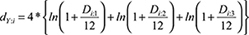

Where:

• d_Y:i is the annual force of dividend or earnings yield for quarter i of year Y.

• D_i:x is the annual dividend or earnings yield, compounded monthly, for month x of quarter i.

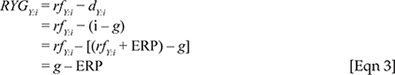
The reverse yield gap

The authors consider the RYG based on equity earnings yields or equity dividend yields. Contemporary corporate finance concepts recognise that dividends are a tool that can be manipulated by companies, discussed in 'the re-emergence of the positive yield gap' section and the 'modelling gross domestic product' section (Berk & DeMarzo 2007; Leary & Michaely 2011). Thus, the authors a priori believe that the RYG based on earnings yields should be superior at forecasting GDP and inflation, as they are a truer reflection of the current state of the equity market.

The RYG measures are calculated as follows: RYG_Y:i = rf_Y:i − d_Y:i

Where:

• RYG_Y:i is the value of the reverse yield gap for quarter i of year Y.

• rf_Y:i is the annual force of return on the government bonds for quarter i of year Y.

• d_Y:i is defined in the 'earnings and dividend yields' section.

Using the results given by Fukui and Kamiyama (2015), the RYG can be expanded. This can be done by assuming that when the market is in equilibrium the return on an equity investment is given by:

and

Where:

• i is the required force of return on the equity investment.

• d_Y:i is defined in the 'earnings and dividend yields' section.

• g is the expected future force of dividend or earnings growth.

• rf_Y:i is defined above.

• ERP is the equity risk premium.

The RYG can then be expressed as:

 

The history of the reverse yield gap

The emergence of the reverse yield gap

Before the early 1960s, both globally and in South Africa, it was generally true that the dividend yield on domestic equity was greater than that on conventional government bonds (Jesse 1977). At that time, Jesse (1977) states, this was thought to be a logical norm as it reflected the overriding view that equities were riskier than government bonds. But as disclosure and accounting standards began to improve, along with better management practices and tighter stock market regulation, the general riskiness associated with equities began to diminish (Jesse 1977).

Business cycles became less pronounced and investors perceived a future with greater economic growth, which in turn meant greater dividend growth (Jesse 1977). Investors were thus prepared to accept a lower initial dividend yield on equities than on government bonds with the expectation that dividend income would at some point grow to outstrip that from the fixed income bonds and, hence, the yield gap turned negative and the RYG emerged (Jesse 1977).

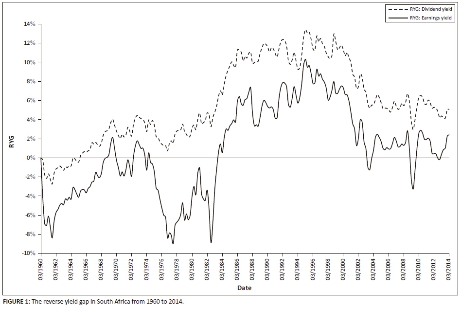
In Figure 1 it can be seen that the dividend yield RYG became positive in South Africa at around 1960, while the earnings yield RYG only became positive later at around 1983. This unusual phenomenon was observed in Sealy and Knight's (1987) empirical investigation into dividend policy influencing share prices on the Johannesburg Stock Exchange. Sealy and Knight (1987) concluded that, over the period 1973-1981, South African listed companies that paid a larger proportion of their profits as dividends had to generate greater returns to shareholders, implying that shareholders preferred profit retention. A plausible explanation is that South Africa taxed dividends during that period.³ General corporate finance theory suggests that companies paying taxable dividends would have to generate higher pretax returns to result in the same after tax position as companies that retain more of the profits, effectively incentivising profit retention (Berk & DeMarzo 2007).

The re-emergence of the positive yield gap

Since the financial crisis of 2008, developed countries once again experienced negative earnings yield RYGs (Fukui & Kamiyama 2015). As can be seen in Figure 1, however, the RYG in South Africa experienced only a few negative spikes in the earnings yield RYG.

The RYG based on dividends yields appears to be smoother with less extreme dips than that of the RYG based on earnings yields. The likely explanation for this is dividend smoothing that describes a company's practice of infrequently changing dividends, and generally upwards only, irrespective of the level of annual earnings (Berk & DeMarzo 2007; Leary & Michaely 2011).

 

In-sample linear modelling

The linear models

To investigate whether or not there is a relationship between the RYG and future inflation or real GDP, linear models were constructed in a similar method to Duarte, Venetis and Paya (2005):

Where:

• is the annual force of either inflation or real GDP as defined in the 'data' section.

• RYG_t−l is the value of the reverse yield gap measure at time t - l, where l is the lag parameter in quarters.

• γ₀ and γ₁ are the intercept and slope values to be estimated.

• ε_t is the random error term associated with the value of at time t. It is assumed that the mean of ε_t is 0 and the variance is some constant σ² for all t.

The model coefficients were estimated for a number of different prediction horizons where k took on values of 1, 2, 3, 4, 5, 6, 8 and 12 quarters. For each different value of k the model was run assuming values for the lag parameter (l) of 0, 1, 2, 3, 4, 5, 6 and 7 quarters. These values for k and l are similar to those tested by Duarte, Venetis and Paya (2005).

For clarity, when using a lag of 0 in the linear model defined by Equation 4, one is using the current value of the RYG to forecast the growth in GDP over the next k quarters.

For the remainder of this article, the RYG based on earnings yields will be denoted by RYG_EY, and by RYG_DY when based on dividend yields.

Comparative model statistics

In order to narrow down the set of considered models, the authors choose models for each value of k over the different values of l that minimises the Akaike information criterion (AIC).

The significance of the RYG measures as predictor variables is measured using Newey-West standard errors to test for the significance of the slope parameter estimate, (Duarte, Venetis & Paya 2005).

The R² measure and the root mean squared error (RMSE) are indicators of goodness of model fit. One of the arguments against the use of the RMSE is that it is not a good indicator of the average performance of a model as it places a higher weighting on larger absolute error terms (Chai & Draxler 2014). The authors of this article, however, suggest that in some cases this may be advantageous as it allows the measure to more accurately expose differences between different model fits. Furthermore, when forecasting GDP and inflation, the authors are interested in the models being able to predict the sudden and sharp changes in GDP and inflation that may happen in reality and thus feel the RMSE is appropriate as models that fail to capture these sharp changes should be penalised.

Modelling gross domestic product

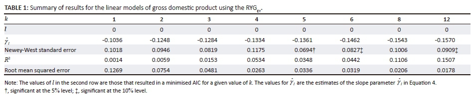
Table 1 and Table 2 summarise the results for fitting the linear models to the real GDP data over the period 1960:1 to 2014:1.

For both RYG measures, the value of the lag parameter that minimises the AIC for all values of k is 0. This indicates that at any time t, the value of the RYG at that time is the best at explaining what GDP growth will be over the next k quarters.

There are two interesting results to take note of. First, all of the slope parameter estimates are negative. When considering Equation 3, a high RYG should indicate a high expected rate of future dividend or earnings growth, relative to the equity risk premium. The authors thus expected that a high expected future growth rate in equity yields, g, should indicate an expectation of high future profits and, hence, ceteris paribus, higher GDP growth. The results seem to indicate the opposite. A possible reason could be that an increase in the RYG is more attributable to a decreasing equity risk premium rather than a large value for g. This would be consistent with a change in market perception that equities have become less risky, for example the positive structural changes to South Africa's economy following democracy in 1994 (Habib & Padayachee 2000). An alternative reason for the apparently contradictory result is that investors' expectations of future market conditions are flawed and hence the expected future growth, g, implied by the RYG does not align with the growth that happens in reality. The simplest reason; however, is that the g term indicates expected growth over a longer term than is tested in this article, that is, longer than 12 quarters ahead, and that if a longer term were tested the nature of the relationship between the RYG and GDP would change.

The second interesting result is that all of the model statistics used indicate that the RYG_DY is better at explaining the GDP data than the RYG_EY. This is unexpected since, as mentioned in the 'reverse yield gap' section, earnings yields are less open to direct manipulation. A possible reason for this result is the 'dividend signalling hypothesis' that states that managers declare dividends on the basis of future expectations in earnings, rather than current earnings that may be distorted through, for example, a once-off large expense (Berk & DeMarzo 2007). This forecasting approach may therefore be a better match for future actual levels of GDP growth.

The general pattern of results for the two sets of models is the same. The R² and RMSE values indicate that the best fitting models are when k is 12, followed by when k is 8 and then 4.

It appears that the best model fits occur when modelling GDP growth over 12 quarters (3 years) ahead, with the overall best model being that for the RYG_DY. This model explained 31% of the variation in the 12 quarters (3 years) ahead GDP growth over the period of observation.

Modelling inflation

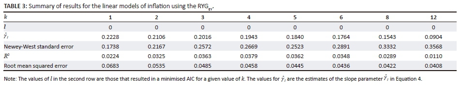
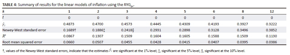
Table 3 and Table 4 summarise the results for fitting the linear models to the inflation data.

Again the value of the lag parameter that minimises the AIC for all values of k is 0; however, there are some noticeable differences between the inflation and GDP models.

All of the inflation model slope parameters are now positive. One possible explanation for this positive relationship is that if investors believe that inflation is going to increase in the future, but are unsure of the magnitude of this change, this could lead to an increase in demand for inflation protecting assets like equities. This would lead to a decrease in dividend or earnings yields relative to gross redemption yields on government bonds and hence an increasing RYG; see Equation 3. Note, however, that the RYG_EY is not significant in any of the models and the RYG_DY is significant in only the first three.

The maximum R² values for each set of models are generally lower for the inflation models than for the GDP models, again suggesting that the RYG is less efficient at explaining future changes in inflation than GDP growth. Another difference is that the R² values for the inflation models reach maximum values when k is either 4 or 5 quarters as compared to 12 quarters (3 years) for the GDP models. When looking at the RMSE statistics, however, the pattern is similar to that under the GDP models with minimum values when k is 12 and 8.

It is not clear that there is any one best fit model out of the tested models for inflation; however, one can say that the results for the RYG_DY models appear better than those of the RYG_EY.

 

Out-of-sample forecasting

The forecasting model

The out-of-sample forecasting is done by removing from the data the observations from 1996:1 to 2014:1. Linear models for both GDP and inflation of the same form as Equation 4 are then fit to the remaining data and used to make single period ahead forecasts. This is an iterative process in which once a forecast for the one period ahead value has been made, the next observation is added to the model and the parameters re-estimated to forecast the next one period ahead value. The rationale behind following this strategy is that if the SARB were to use the RYG to predict GDP or inflation over the next k quarters, at each subsequent quarter the newly observed market data would be added to their model.

This process is followed for each considered value of k, the forecasting horizon, while the value of the lag parameter, l, is kept as 0. The models are then compared using a RMSE approach applied only to the errors relating to the forecasted data and not to the fitted linear models. Since, for each iteration, the model parameters are re-estimated, the significance of the slope parameters with regard to the Newey-West standard errors will not be considered.

The size of the RMSE value will be somewhat swayed by the absolute values of the observations. Thus, because the scale of the real GDP and inflation underlying data is different, one cannot compare directly the RMSE values between the two sets of models, but rather only between the various models within each GDP and inflation category. A summary of the forecasting results can be seen in Table 5.

 

 

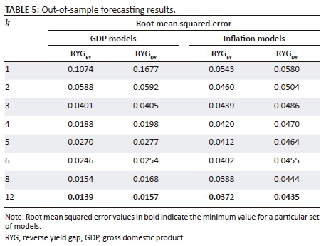
Results for forecasting gross domestic product

For each RYG measure, the minimum RMSE values were obtained when forecasting GDP growth over 12 quarter periods (3 years). This is in line with the results found in Table 1 and Table 2. In contrast with the in-sample modelling, however, the RYG_EY models outperform the RYG_DY in terms of the RMSE statistic for all values of k and this requires further consideration.

When comparing the error terms for the RYG_EY and RYG_DY forecasting models where k is 12, it is seen that up to the end of 2003 the RYG_EY model outperforms the RYG_DY model at every point and vice versa after 2003. By then observing the GDP data it is noted that from 1996:1 up to the end of 2003, there is a general upward trend in three-year GDP growth rates, after which there is a general downwards trend.

In the 'forecasting gross domestic product over different economic periods' section, the authors investigate the nature of the relationship between the RYG_EY and future economic growth during periods of upwards or downwards growth. The results indicate that the RYG_EY has an improved linear relationship with future GDP growth during upwards economic cycles and little, if any, linear relationship with future GDP during downwards cycles. By reference to the upwards and downwards economic cycle periods obtained from the SARB, at least 74% of the months over this forecasting period are considered to be in an upwards cycle, whereas for the data before this period, only 57% are contained in upwards cycles.

It is also observed that the period over which the RYG_DY performs at its worst compared to the RYG_EY is during the time of the Asian economic crisis, and that over this period there was actually a general pattern of increasing three-year economic growth in South Africa. It is possible that market participants expected this crisis to result in a lower than observed growth rate in South Africa and, as dividends are set by companies, this incorrect expectation was more pronounced in the RYG_DY than in the RYG_EY.

Overall it is likely that the rapid economic growth experienced in South Africa over the period 1996:1-2013:4 resulted in the better performance of the RYG_EY model compared to the RYG_DY model over this period.

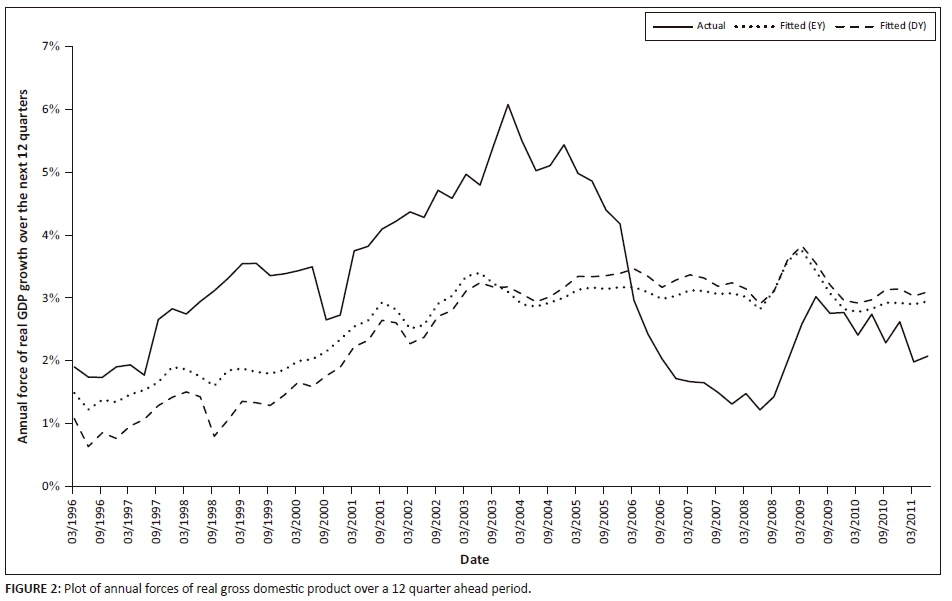
Figure 2 shows a graph of the best fit models for forecasting GDP. Note that each point represents the force of GDP growth over the next 12 quarters (3 years), not the growth experienced at that date.

There appears to be little difference between the two models, except over the period 1996 to around 2001. Both forecast models seem to follow the general trend of GDP growth but do not exhibit the extreme peaks and troughs as found in reality. This is disappointing, since what is of key interest when forecasting GDP growth is to be able to predict economic troughs and peaks. The SARB in particular would probably be interested in modelling the extreme possible future outcomes as a result of changes in current economic conditions. Of particular concern is the steep decline in actual GDP growth over 2005-2009 where both forecast models seem to show almost level growth over this period.

It is noteworthy that the forecasts under the EY and DY models are similar. Brill and Toerien (2011) found that directors in South Africa generally believe that reducing dividends leads to negative consequences and that maintaining consistency with historic dividend policies is important. There is evidence of dividend smoothing in Figure 1; however, the similarity of the model results suggests that dividends are not smoothed to such an extent that the underlying earnings' patterns are masked.

Overall, it appears that while there may be some relationship between future GDP growth and the value of RYG_EY and RYG_DY, these variables alone are not sufficient to reasonably assist the SARB in monetary policy decision-making.

Results for forecasting inflation

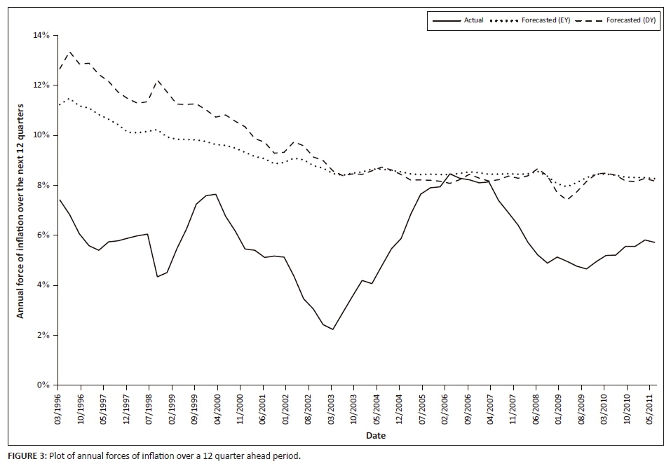
The models that performed best at forecasting inflation were again the models with a forecasting horizon of 12 quarters. This is interesting as the results in Table 3 and Table 4 suggest that neither RYG measure is significant when k is 12; however, the results are consistent with the RMSE minimum values from the original linear models. Again, the RYG_EY models outperformed the RYG_DY models for all values of k when forecasting inflation.

Figure 3 shows the graph for the two best inflation forecasting models and can be interpreted in a similar way to that explained for Figure 2.

From Figure 3 it is not particularly clear that either of the models reasonably follows the actual inflation observations. The forecasts do not appear to follow the general trend of inflation, nor do they capture the cyclical nature of actual inflation. As a result of the relatively poor fits, inflation will not be modelled further in this article.

 

Forecasting gross domestic product over different economic periods

Economic cycles

Davis and Fagan (1997) state that cyclical effects play a large role in economic growth and it is important to take into account these effects when using financial spreads to forecast economic growth. The linear relationship between the RYG and future real GDP growth in South Africa is therefore modelled separately over upwards business phases and downwards business phases. The dates for these different periods were obtained from the SARB Quarterly Bulletin for June 2015⁴, where business cycles are identified by analysing business cycle indicators, of which a description can be found in Venter (2011) and Bertolis and Hayes (2014).

Method and model descriptions

The business phases begin and end on a monthly basis; thus, the quarterly data used in this study is allocated to a specific business cycle period only if the full quarter considered is contained within that cycle. Similarly, when considering the GDP growth over a period of k quarters, this observed growth value is only allocated to a specific cycle if the entire k quarters under consideration are contained in that cycle period. This is to avoid ambiguity around interpreting results where some observations contain growth incurred in both upwards and downwards phases.

The modelling process followed is the same as that in the 'in-sample linear modelling' section with the same model structure as Equation 4. Linear models are constructed for the upwards and downwards phase data for each of the forecasting horizons, k, and lag parameter values, l. Due to the fact that the RYG_EY models performed better under the out-of-sample forecasting of GDP growth, the models in this section only consider the RYG_EY as a predictor variable.

Note the developed models for each different value of k are conditional models in the sense that each will indicate the relationship experienced during upwards (downwards) business cycles between the RYG_EY some l quarters ago and the growth in GDP over the next k quarters, given that the business phase remains an upwards (downwards) phase over the next k quarters.

In-sample modelling over different business cycles - results

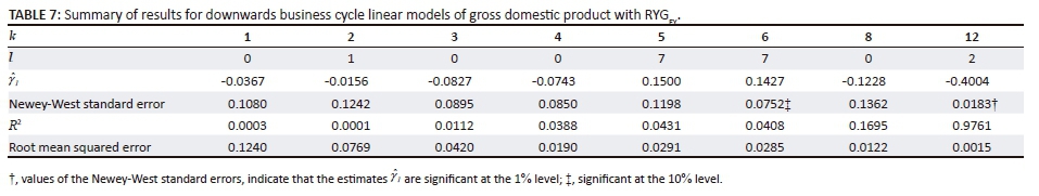
The lag parameters that minimise the AIC values are no longer all 0 as was the case in Table 1 and Table 2. Table 6 seems to indicate that a lag parameter of 1 or 6 is generally most appropriate when forecasting GDP over an upwards business cycle, while in Table 7, the lag parameter of 0 is the most common.

While the majority of slope parameters are negative, those for the downwards phase models where k is 5 and 6 are positive; however, only the value at k equal to 6 is significant at a 10% level. This positive relationship implies that an increase in GDP is associated with an increase in RYG_EY; this is what was expected as per the explanation in the 'modelling gross domestic product' section. This may suggest that during economic down cycles the RYG_EY and GDP growth have a positive relationship; however, the results are not conclusive and in fact it appears more likely that these two positive parameters are anomaly occurrences.

The large R² value of 97.61% when k is 12 for the downwards phase models is likely attributable to the fact that the downwards phases were in general much shorter than the upwards phases and as a result there were few, seven to be exact, observations of 12 quarter GDP growth during downwards cycles. As such the results for this model cannot be relied upon for credible conclusions. Excluding the results for this model, the results for the upwards phase models are generally better than those for the downwards phase models, and in fact the lack of significance of slope parameters and poor R² values indicate there may not even be a relationship between the RYG_EY and GDP growth during periods of economic downturn. During upwards periods, the best R² and RMSE models are where k is 12 and 8. Note that these results are an improvement on the results for the RYG_EY models over the full period of investigation (see Table 1) and the R² value of 42.77% when k is 8 is the best obtained over this entire study.

Out-of-sample forecasting over different business cycles

A general rule of thumb is that for a model to be able to credibly forecast results it should contain at least 20 observations (Clemen & Winkler 1986). The upwards phase forecasting models were thus developed by building an initial model on the first 20 observations and then iteratively forecasting the next one quarter ahead GDP result, as explained in the 'out-of-sample forecasting' section. Due to fewer observations being available for the downwards phase forecasting models, the initial models were developed on the first 15 observations. Note that no forecasting model was developed for the downwards data when k is 12 as a result of only having seven observations. Table 8 summarises the results of the forecast models.

 

 

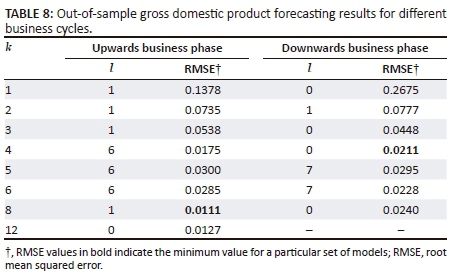
The minimum RMSE for the upwards phase models is obtained when k is 8 (2 years) and l is 1; this is an improvement on the minimum value of the RMSE for the RYG_EY when considering the entire data set and indicates that there may be a stronger linear relationship during upwards economic cycles. For the downwards phase models the minimum RMSE value occurs when k is 4 (1 year) and l is 0, but this is not an improvement on the results for the full data set and again suggest that the linear relationship is weaker during downwards economic phases.

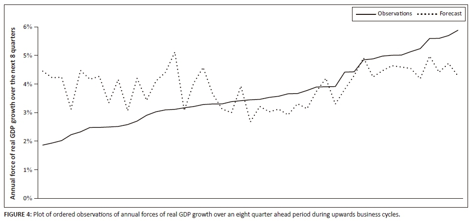
Graphs of these two best forecast models are given in Figure 4 and Figure 5. Note that there are no dates on the horizontal axes as the data are grouped over all upwards or downwards phases and hence do not always occur over consecutive dates. Instead, the actual observations of GDP growth have been plotted in increasing order along with the corresponding forecasted value at each point. If the forecasting model is accurate it should produce a similar upwards sloping graph to that of the observed GDP.

Neither of the above graphs shows any signs of the forecasting models having a reasonable forecasting ability, and in fact neither seems to even produce a graph with a clearly upward sloping trend throughout. This indicates that it is unlikely that the RYG_EY as a linear predictor of GDP growth will be a reasonably useful single tool to the SARB when considering the use of different models over upwards and downwards business cycles.

 

Conclusion

Forecasting economic growth

A high RYG should indicate a high expected rate of future dividend or earnings growth, relative to the equity risk premium. The authors therefore reason that a high expected future growth rate in equity yields should indicate an expectation of high future profits and hence, ceteris paribus, higher GDP growth. From the in-sample linear modelling, however, all of the slope parameter estimates are negative indicating the opposite, which is unexpected.

When considering the linear relationship between the two RYG measures and GDP growth over the entire investigation period, the RYG_EY models have superior out-of-sample forecasting abilities and the relationship seems strongest with a lag parameter of 0 and a forecasting horizon of 12 quarters (3 years).

The forecasted models, however, did not capture the extreme changes in GDP growth that sometimes occur in reality. This is disadvantageous as these extreme values are likely the ones the SARB is most interested in predicting.

When modelling GDP growth over different business cycles it was found that the linear relationship between the RYG_EY and GDP growth is strongest during upwards economic cycles, although when looking at the out-of-sample forecasted model, this linear relationship does not appear strong.

The RYG_EY may still be useful to the SARB since it appears to capture some aspects of the general trend in GDP growth and it may be found that the information contained within the RYG_EY, although insufficient on its own, could replace a number of variables in the SARB's core model without any significant loss in forecasting ability.

Forecasting inflation

There does not appear to be any linear relationship between future inflation and either of the two RYG measures. The minimum RMSE value was found when forecasting inflation over 12 quarters (3 years) with the RYG_EY value at the current time t; however, this model did not appear to follow even the general trend of inflation over the investigation period.

Further research

The following areas of research could be pursued to further the results found in this article:

• Testing the RYG as a predictor of real GDP growth alongside other variables already considered by the SARB.

• Testing if the forecasting ability of the RYG could be improved by use of non-linear models, such as was done by Duarte, Venetis and Paya (2005).

• Testing the ability of the RYG to forecast inflation during different times in the economic or inflationary cycle.

 

Acknowledgements

The authors thank Mr G. Haltmann for assisting with some of the coding that was used to compute the models and model statistics. We also thank the anonymous reviewers for their helpful comments.

Competing interests

The authors declare that they have no financial or personal relationships that may have inappropriately influenced them in writing this article.

Authors' contributions

K.A.G. was the principal author, who instituted the study and undertook initial analyses and inferences. M.G.H. supervised the principal author and co-wrote additional analyses and inferences, with supporting references

 

References

Armah, N. & Swanson, N., 2011, 'Some variables are more worthy than others: New diffusion index evidence on the monitoring of key economic indicators', Applied Financial Economics 21(1/2), 4360. https://doi.org/10.1080/09603107.2011.523188        [ Links ]

Aron, J. & Muellbauer, J., 2007, 'Review of monetary policy in South Africa since 1994', Journal of African Economies 16(5), 705-744. https://doi.org/10.1093/jae/ejm013        [ Links ]

Berk, J. & Demarzo, P., 2007, Corporate finance, Pearson Education, Inc., Boston, MA.         [ Links ]

Bertolis, D. & Hayes, M., 2014, 'An investigation into South African general equity unit trust performance during different economic periods', South African Actuarial Journal 14, 73-99.         [ Links ]

Brill, E. & Toerien, F., 2001, Dividend policy in South Africa: A survey of financial directors of JSE listed companies, UCT Graduate School of Business, Cape Town.         [ Links ]

Chai, T. & Draxler, R., 2014, 'Root mean square error (RMSE) or mean absolute error (MAE)?', Geoscientific Model Development Discussions 7, 1525-1534. https://doi.org/10.5194/gmdd-7-1525-2014        [ Links ]

Clay, R. & Keeton, G., 2011, 'The South African yield curve as a predictor of economic downturns: An update', African Review of Economics and Finance 2(2), 167-193.         [ Links ]

Clemen, R.T. & Winkler, R.L., 1986, 'Combining economic forecasts', Journal of Business & Economic Statistics 4(1), 39-46.         [ Links ]

Davis, E. & Fagan, G., 1997, 'Are financial spreads useful indicators of future inflation and output growth in EU countries?', Journal of Applied Econometrics 12(6), 701-714. https://doi.org/10.1002/(SICI)1099-1255(199711/12)12:6<701::AID-JAE456>3.0.CO;2-9        [ Links ]

Duarte, A., Venetis, I. & Paya, I., 2005, 'Predicting real growth and the probability of recession in the Euro area using the yield spread', International Journal of Forecasting 21, 261-277. https://doi.org/10.1016/j.ijforecast.2004.09.008        [ Links ]

Fukui, Y. & Kamiyama, N., 2015, Risk premium, price multiples, and 'reverse yield' gap, SSRN Scholarly Paper No. ID 2290823, SSRN, Amsterdam.         [ Links ]

Habib, A. & Padayachee, V., 2000, 'Economic policy and power relations in South Africa's transition to democracy', World Development 28, 245-263. https://doi.org/10.1016/S0305-750X(99)00130-8        [ Links ]

Jesse, R., 1977, 'The reverse yield gap and real return', Investment Analysts Journal - Investment Analysts Society of Southern Africa 10, 37-38.         [ Links ]

Maio, P., 2013, 'The 'fed model' and the predictability of stock returns', Review of Finance 17(4), 1489-1533. https://doi.org/10.1093/rof/rfs025        [ Links ]

Fama, E.F., 1970, 'Efficient capital markets: A review of theory and empirical work', The Journal of Finance 25(2), 383-417. https://doi.org/10.2307/2325486        [ Links ]

Finnerty, J.E., 1976, 'Insiders and market efficiency', The Journal of Finance 31(4), 1141-1148. https://doi.org/10.1111/j.1540-6261.1976.tb01965.x        [ Links ]

Leary, M.T. & Michaely, R., 2011, 'Determinants of dividend smoothing: Empirical evidence', The Review of Financial Studies 24(10), 3197-3249. https://doi.org/10.1093/rfs/hhr072        [ Links ]

Nobili, A., 2006, 'Assessing the predictive power of financial spreads in the euro area: 'Does parameters instability matter?', Empirical Economics 33(1), 177-195. https://doi.org/10.1007/s00181-006-0098-x        [ Links ]

Sealy, N.R. & Knight, R.F., 1987, 'Dividend policy, share price and return: A study on the Johannesburg Stock Exchange', The Investment Analysts Journal 16, 33-47.         [ Links ]

Smal, D., Pretorius, C. & Ehlers, N., 2007, 'The core forecasting model of the South African Reserve Bank', South African Reserve Bank Working Paper No. 07-02, SARB, Cape Town.         [ Links ]

Timmermann, A. & Granger, C., 2004, 'Efficient market hypothesis and forecasting', International Journal of Forecasting 20(1), 15-27. https://doi.org/10.1016/S0169-2070(03)00012-8        [ Links ]

Venter, J., 2011, 'Business cycles in South Africa during the period 2007 to 2009', South African Reserve Bank: Quarterly Bulletin 260, 61-66.         [ Links ]

 

 

Correspondence:
Mark Hayes
mark.hayes@curtin.edu.au

Received: 27 July 2016
Accepted: 28 May 2018
Published: 16 Aug. 2018

 

 

1 . This information was obtained from the South African Reserve Bank's official website and can be found at: https://www.resbank.co.za/MonetaryPolicy
2 . The SARB online database can be accessed at the following address: https://www.resbank.co.za/Publications/QuarterlyBulletins/Pages/QBOnlinestatsquery .aspx
3 . Deloitte, Haskins & Sells (1987). A guide to the recommendations of the Margo Commission of Inquiry into the tax structure of the Republic of South Africa.
4 . The published dates for the South African business phases can be found on page S-157 of the Statistical Tables section of the SARB Quarterly Bulletin June 2015, which can be viewed at: https://www.resbank.co.za/Publications/QuarterlyBulletins/Pages/QuarterlyBulletins-Home.aspx