ARTICLES

 

Fair pricing, and pricing paradoxes

 

 

Barbara Swart

Department of Decision Sciences, University of South Africa

 

 

---

ABSTRACT

The St Petersburg Paradox revolves round the determination of a fair price for playing the St Petersburg Game. According to the original formulation, the price for the game is infinite, and, therefore, paradoxical. Although the St Petersburg Paradox can be seen as concerning merely a game, Paul Samuelson (1977) calls it a "fascinating chapter in the history of ideas", a chapter that gave rise to a considerable number of papers over more than 200 years involving fields such as probability theory and economics. In a paper in this journal, Vivian (2013) undertook a numerical investigation of the St Petersburg Game.
In this paper, the central issue of the paradox is identified as that of fair (risk-neutral) pricing, which is fundamental in economics and finance and involves important concepts such as no arbitrage, discounting, and risk-neutral measures. The model for the St Petersburg Game as set out in this paper is new and analytical and resolves the so-called pricing paradox by applying a discounting procedure. In this framework, it is shown that there is in fact no infinite price paradox, and simple formulas for obtaining a finite price for the game are also provided.

Key words: discounting, fair no-arbitrage price, martingale probability measures, pricing paradox

JEL: A1, 2 C00, 6

---

 

 

1 Introduction

The famous St Petersburg Game pricing paradox has, over the last 275 years, occupied many great minds, including economists such as Paul Samuelson and J.M. Keynes, and has directly or indirectly influenced some of the work of mathematicians such as Borel (1949), and even John van Neumann.

1.1 The St Petersburg Game (PG)

The paradox surrounding this very famous game goes back to the early 1700s. Bernoulli presented the paradox to the St Petersburg Academy in 1738, and it has attracted attention ever since. Samuelson (1977) states that the paradox "enjoys an honoured corner in the memory bank of the cultured analytic mind". The PG concerns a single game (between a player and a bank or casino) which may last arbitrarily long, has infinite expected payoff and, according to the paradox, an infinite price.

One play of the game proceeds as follows: A coin is flipped repeatedly at times t = 1, 2, 3, ... until the first tails T appears, when the payoff is paid out and the game ends. The accumulated payoff St, if the game ends at time t, consists of doubling up initial amount S0 = 1 for each successive heads H, and has possible values S_t= 2; 2²; 2³; ... 2^t ; ..., with respective probabilities 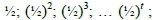so on. The run of heads can be arbitrarily long, and the expected payoff for one play of the PG is infinite:

The argument for finding the fair price FP for the St Petersburg Game given in the literature (Bernoulli 1738; Samuelson 1977; Mackinnon 1990; Vivian 2013) then proceeds as follows: A fair price implies that the expected profit should be zero. That is:

If one writes:

it follows that:

This pricing argument, together with (1.1), then implies that the "fair" price FP is infinite:

What makes the PG so interesting is that the length τof the St Petersburg Game, that is, the number of Hs before T appears, is a random variable. The PG may have an arbitrarily long run, but may also end after only 1 coin flip, with payoff 1, or after 2 flips with payoff 4, and so on. It is rather a shock to calculate the expected value of the length τof the St Petersburg Game. Noting that τ= 1 with probability /½; τ= 2 with probability (½)²; and so on, it follows that:

The paradox is this: It appears that the correct, fair price is infinite, but no player will pay this upfront for an expected, infinite final payoff, especially for a game that is expected to end after 2 tosses. Also, the probability of winning amount 2^τ for very long τis only (½)^τ" - for example, there is a 0.098 per cent chance of winning 1,024 units of money and about a 0,0000009 per cent chance of winning a million units.

Is there a way out of the paradox? An immediate objection to (1.1) and (1.5) could be that an infinite amount of money has no meaning in a real-life situation. However, this does not resolve the paradox on a theoretical level where economics and mathematics apparently show that the price of the PG is infinite. For the sake of investigating the paradox, it is therefore assumed that player and bank have unrestricted resources.

In Sections 1.2 to 1.3, we present some important observations on the St Petersburg Paradox, observations that are not mentioned elsewhere in the literature.

1.2 Mathematical issues

The pricing argument in respect of (1.2) to (1.4) is flawed mathematically.

For any random variable X, the expression E[X] = ∞ may be defined in probability theory, but working with infinity needs care. For example, E[X - Y] = E[X] - E[Y] is not true if both E[X] = œ and E[Y] = ∞ (Durrett, 1996). This simple fact (though not mentioned in the literature relating to the PG) already dispels the "paradox" presented by the simplistic reasoning in Equations (1.2) and (1.3). Writing E[Payoff - Price] = E[Payoff] - E[Price] implies that either E[Payoff] or Price must be finite. And, if either is finite, then, by assumption (1.2), they must be equal and both will be finite. Therefore, applying fair pricing and Formula (1.3) means there can be no paradox: both expected payoff and price must be finite. An appropriate model for the pricing of our games should reflect this, and relationships (1.2) to (1.4) do not.

1.3 Issues of time and risk

Firstly: Even if one is guaranteed to have a very long run of successive Heads, it makes no economic sense to pay an infinite (or even finite but large) amount now, for a large amount paid out only after a very long time.

Secondly: Suppose it is agreed that the game lasts for a maximum of K flips with a maximum possible final payoff of 2^K (if there are K successive Heads). Then:

The "fair" price for this truncated game then has a finite value K and there is no apparent paradox. But, to break even in this truncated PG, the player must have an immediate run of X number of successive Heads such that 2^X> K. Solving for X gives us: X > log₂K. As an example, assume the rule is that the game stops after K = 2⁸ flips, so that the price is 2⁸. An immediate run of at least log₂2⁸ = 8 successive Heads is needed just to break even, and the probability of this happening is only (½)⁸= 0.39 per cent. The probability of making a profit of only 4 units is about 0.01 per cent (0.0001). This is too risky for the player.

From the point of view of the bank, it is unlikely that the PG can be hedged by a portfolio with the same outcome space and price K. There is a probability - however small - that the bank may have to pay out a massive amount of 2^K, and this may be far too risky for the bank.

In conclusion: The economics of "infinite payoffs and prices", without taking time and risk into consideration, makes little sense. The "fair" pricing formula (1.4) for St Petersburg games does not appear to satisfy all the criteria of fair pricing. This brings us to the concepts of no arbitrage, discounting, and true fair pricing, which we will show resolves the paradox.

1.4 Fair pricing, no arbitrage, and discounting

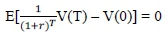
The "no-arbitrage" assumption is basic to all pricing theory. It is also known as the "no-freelunch" assumption and implies that there should be no expectation of riskless profit when entering into a financial transaction. The expected present value (PV) of the profit must be zero in order to ensure a fair price (Pliska, 1997; Björk, 2004):

The PV of a quantity is obtained by discounting it to time t = 0 or when the price is paid, most commonly using factor , where r is the benchmark risk-free bank rate and t indicates time.

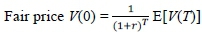
This then yields the true fair pricing formula: For any investment Vover time interval [0, T], its fair price V(0) is determined from (1.8) by relationship:

This is

The important roles of time and discounting in ensuring a risk-neutral price are now clear. None of the previous papers that deal with the St Petersburg Game mention this. The present contribution is to use the above insights and replace the simplistic and incorrect "fair" pricing of section 1.1 with a mathematically and economically sound model, along the lines implied by (1.8).

In summary: The "fair" pricing formula (1.4) for St Petersburg games does not satisfy all the criteria in respect of fair pricing. Here, the problem will be placed within a martingale framework and it will be shown how to apply discounting in particular to the pricing model for the PG so that time value and risk considerations are introduced and fair pricing can be shown to yield finite prices. The notion of a pricing paradox is dispelled, and a formula for the actual value of the (finite) fair price of a game will be given.

 

2 Literature review

Samuelson (1977) provides a detailed discussion of the history of the game and of the efforts at solving the paradox. This is in effect a literature review in itself. Vivian (2013) also provides a good overview. The next sections give brief summaries of some of the attempts at resolving the St Petersburg Paradox.

2.1 Utility functions

Some authors (see Samuelson's discussion (1977)) suggest the use of an equilibrium framework and utility functions to determine a price that would satisfy both agents, that is, a utility price rather than a fair price. The basic idea is that players base decisions on an expected (concave) utility function of wealth rather than on the expected value (a linear function) of wealth. This presents one way of resolving the pricing paradox and reveals fascinating applications of utility theory (Menger, 1934).

We prefer to stay within the fair price framework in which the pricing paradox was originally formulated.

2.2 Truncating the game

One can consider the variant St Petersburg game with the rule (Mackinnan, 1990) that, if pre-specified throw number K still shows Heads (i.e. you have successive HHH ... HH for K throws), you will accept cumulative payoff (2^K) and the game will stop. In other words, the game is restricted to K flips at most (but may, of course, end much sooner). This case was discussed in Section 1.3 above - the "fair" price for this truncated game is finite K (Equation (1.7)) and there is no apparent paradox. But, as pointed out there, problems arise even in this case, and, furthermore, the truncation is not really a satisfactory solution, since it does not apply to the true PG.

2.3 Playing the St Petersburg Game repeatedly

The idea, here, is to consider a large number of plays of the PG, and then take the average value as the price per game. To formalise this framework something like the Weak or Strong Law of Large Numbers is needed. Neither law can be used for the PG, but there is, however, a Weak Law for Triangular Arrays that can be applied to the PG. The discussions in Feller (1945, 1968) and Durrett (1996) provide the solid basis for this method. We give the result without the proof (which can be found in Durrett (1996:44-46): Let Sⁿdenote the cumulative payoff after playing the St Petersburg Game n times. Then it can be shown that , in probability, as n - ∞. This means that, for large n, the average payoff per game, namely , is close to log₂ηin probability.

The price for playing n games is nlog₂n, and the fair price per game, when playing n games, is:

This is an intriguing result. The "fair" price for playing the PG only once (n = 1) is zero. Clearly, no bank will accept this price and will insist on the player playing a larger number of times. The price for playing 2^K times is 2^Klog₂ 2^K = 2^K*K, or K units per game. There is no fixed fair price per game - it all depends on how many games you agree to play. This pushes up the cost of playing. Remember, also, that the convergence leading to result (2.1) is in probability only, and the result is therefore a weak one.

2.4 Simulating the St Petersburg Game

Count Buffon proposed this method as far back as the 18th century (Buffon, 1777). He employed a child to play the game repeatedly and then tabulated the results. According to him, there would always be a finite run of Heads, and, therefore, a finite price and no paradox. Apart from this questionable methodology, both Buffon and D'Alembert (see Samuelson, 1977) made another astonishing statement: They agreed that any probability smaller than, say, 10^-4 could simply be set equal to zero, in this way guaranteeing a finite payoff and price!

More recently, the use of computers has been suggested to simulate and examine the paradox. In this case, a virtual coin is flipped a very large number of times and the payoff is then calculated. The process (game) is repeated a large number of times and the average of payoffs is taken. This value is then offered as the expected final payoff - and thus price - for playing the PG once. This can be seen as a practical implementation of the discussion in Section 2.3.

The paper of Vivian (2013) follows this path and we can compare his computer results with the theoretical price given by (2.1). It appears that his simulated values for the price per game when playing large numbers of times are roughly of the order of the theoretical values predicted by Feller (1945). For example: For 2¹⁰ repeated computer plays, the price per game is 6.84, while Feller's price is 10. See Table 3 in Vivian (2013). All his simulated PGs ended after a finite run of Heads.

Vivian's conclusion is that numerical experiments show that the St Petersburg Paradox is resolved: There is no paradox, since his computer simulations show finite lengths of games, and finite prices can be computed as the average of a large number of plays. Although his paper is very insightful and a valuable way of investigating the paradox, computer experiments still amount to a truncation of the repeated plays after some (however long) time. From a mathematical or statistical point of view, it is also not quite satisfactory to state that a finite number of experiments shows that all PG games will have a finite length. Another problem with the simulation method is that it does not produce a unique, feasible price per game for practical use: Repeating the simulations will yield different payoffs and different prices.

 

3 Research methodology for solving the original St Petersburg Game

The research methodology is to develop the ideas presented in Sections 1.2 to1.4 and to show that the concept of discounting can be used to introduce time value and risk considerations into games such as the PG, which then leads to finite expected payoffs and finite prices. The pricing paradox is thus resolved. We will also attempt to place the problem within a martingale framework.

Fair pricing involves determining the expected values of terminal payoffs, and, in the case of the pricing paradox, includes instances where we have possibly infinite payoffs and infinite exercise times. We first explain pricing concepts in an accessible way, but using the necessary mathematics and correct pricing procedures. These ideas will then be used to give alternative analytical solutions to the St Petersburg Paradox which are not based on numerical experiments such as those of Vivian (2013).

We start with some definitions to set up the general risk-neutral framework for fair pricing in economics and finance - it is essential to understand the foundations of fair pricing, since failure to do so may lead not only to our PG paradox, but also to serious mispricing of financial assets, and may play a role in financial crises.

3.1 The assumption of no arbitrage

As mentioned in Section 1.4, this assumption is the basis of pricing theory. There should be no riskless profit, so that today's price should equal the present or discounted value PV of the expected final payoff.

Discounting is done via a discount factor or discount rate: The PV of a payment made at time t is obtained by discounting it to t = 0 when the price is paid. Usually, a risk-free bank rate r is assumed, and the factor or e^-rt in the case of continuous compounding, is applied to the final payment. For any investment V over time interval [0, T], therefore, its fair price V(0) is determined by relationship:

Note that the final values V(T) are random variables representing all possible outcomes at time T, while V(0) is the deterministic price at time 0 when the transaction is entered into.

It seems obvious that the expected value in (3.1) is taken with respect to the probability measure P, which describes the real-world probability distribution of V at T. However, this is not the case: The fair price is determined by an artificially constructed risk-neutral measure Q which assures zero risk-less profit and is linked to the discounting factor. We discuss this next.

3.2 Martingales

The no-arbitrage condition for a market with risky price process S(t) and risk-free bank rate r is most clearly stated as follows (Pliska; 1997; Björk 2004): There are no arbitrage opportunities if -and only if - there exists a probability measure Q with the following properties:

Note: E^Q[S*(T)|F_t] is the expected value of S*(T), conditional on filtration F at time t. Without going into the mathematics, one can think of the filtration F_tas "information generated by all observed events regarding S up to time t" (Björk, 2004).

Specifically, time-0 fair values or prices are given by:

Statement (3.4) is the "First Fundamental Theorem of Mathematical Finance". In economic terms, it states that today's price is the expected value under measure Q of the discounted future price.

In the risk-neutral (no-arbitrage) Q-world where fair prices are constructed, price processes 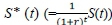are called martingales, and Q is a martingale measure. It is not identical to real- world probability distribution P, but is equivalent to P.

The modern framework for the pricing of financial products is based largely on martingale methods. Measure Q is unique if - and only if - the market is complete. (In a complete market, investments can be hedged or replicated so that, if two contracts or games V₁and V₂have the same final payoffs, they will also have the same prices.)

In the case of an incomplete market where there is no unique Q and the seller of a contract cannot hedge the contract, finding Q is not just a mathematical exercise. The choice of Q is equivalent to choosing the market price of risk. One can do no better than quote Björk (2004:221): "In an incomplete market the price is also determined, in a nontrivial way, by aggregate supply and demand on the market. Supply and demand are, in turn, determined by the aggregate risk aversion on the market, as well as by liquidity considerations and other forces." These remarks are important, since it is not clear that the St Petersburg Game (a possibly perpetual contract) can be hedged by the bank or casino (see Section 1.3).

The framework presented above will form the basis of our solution to the pricing paradoxes. To summarise the important points: Discounting is necessary, since pricing is not absolute but relative; time plays a role; no-arbitrage pricing should imply finite prices even for perpetual products; and, especially in incomplete markets, the risk preferences of parties are needed to determine the price. See also Bru, Bru and Chung (2009) and Mazliak and Shafer (2009) for discussions on martingales.

 

4 Results: Resolving the St Petersburg Paradox

We consider the original St Petersburg Game, played once, as discussed in the Introduction, Section 1.1.

4.1 A fair solution to pricing paradoxes using discounting

Our submission is that the usual formula (1.4) used in the literature on games does not give a fair price for games with a large or possibly infinite time horizon, and that the pricing principles with discounting discussed in Section 3 should be followed. Looking at pricing formulas (3.1) and (3.4), it is clear that discounting is an essential component of fair pricing, but this is ignored in the literature on games, as shown by the application of (1.4). The fair, no-arbitrage price is determined by the present values of expected payoffs, and the payoff process under consideration should be as in definition (3.3):

where S_tis the accumulated payoff considered in Section 1.1, and βis a discounting or deflating factor.

The discounter βcan be negotiated by both player and bank. (In financial portfolio or asset pricing, β= with r the benchmark risk-free bank rate.)

Factor βshould be positive (β> 0) and satisfy β< 1 for all terms, or for all but a finite number of terms where one can take β= 1 if one so wishes (see (4.2) below).

The function of parameter βis to reflect risk (including market price of risk) and/or time considerations. If it is felt that initial terms need not be deflated, since the first (say K) flips do not add up to much time, a better choice for βcould be:

Or, more generally:

More sophisticated choices for ß(t) can be negotiated between player and bank.

4.2 A finite price for the St Petersburg Game

Payoffs for the PG should be discounted - in its simplest form, payoffs at each step t are discounted with factor ß^twhere ß < 1. The fair price for the St Petersburg Game is then:

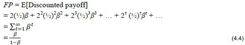
The fair price is finite and fixed once the value of ß has been negotiated.

(Formula (4.4) also gives the price of a perpetual annuity of a stream of unit payments with

Discounting makes sense of both the mathematics and economics for cases of large or infinite time and gets rid of any "infinite price paradox". If the agents involved cannot agree on a value for ß, there is simply no supply and no demand, and, therefore, no game. Pricing formula (4.4) has a simple analytical form and provides, at least theoretically, a more satisfying solution to the "infinite price paradox" than just limiting the wealth of players and banks or the number of flips of the coin.

Formula (4.4) can also be made more dynamic, as suggested above, by applying different discount factors over different time periods. For example, the fair price using discounting factor (4.2) is:

and, using (4.3) as the discounting factor:

4.3 The price using a martingale measure adapted to β

In the above discussion, probability measure Q = {½; ½} was used as a risk-neutral measure. The risk-neutral measure and the discounting factor are usually linked, as shown in the martingale theory for Section 3.2, Equation (3.4). Different risk-neutral measures are also possible in incomplete markets.

The accumulated payoff process S(t) can be represented by a tree structure (Pliska, 1997), and one can then easily show that the following martingale property (the one-step version of (3.2)) holds at each t:

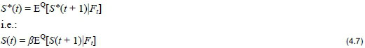
Martingale measure Q = {qu; qd}, consistent with deflator ß, can now be constructed: Application of (4.7) at any time t, together with the probability condition, respectively yields equations:

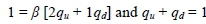
The solution is:

Since we must have both q_u > 0 and q_d > 0, the restriction on βis: ½ <β< 1.

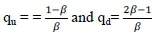
Then, for ½ <β< 1, we have, for the simplest pricing case:

FP = E[Discounted payoff]

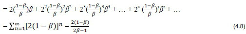
Negotiating a specific value of βimplies a new risk-neutral probability measure.

The fair price of 2 is thus consistent with martingale measure {q_u; q_d} = {½; ½}.

The bank will probably not be happy with this price and will want to negotiate a value of βcloser to V in pricing formula (4.8)!

4.4 Other simple solutions to the paradox?

Our final suggestions for resolving the pricing paradox are very simple, and are also not mentioned in the literature. Suppose that the notion of discounting is ignored and we return to the original Formula (1.4). In Equation (1.6), we saw that the expected time for the game to stop is τ= 2, and so the expected payoff for the PG should be no more than the expected time 2-payoff, namely E[S₂]. Since 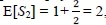, the "fair" price FP according to (1.4) should be:

This accords with the price given in (4.9) above.

It is also interesting to consider a variation of the original pricing formula (1.4) using utility functions U(W), where W is the final payoff. Thus, assume formula:

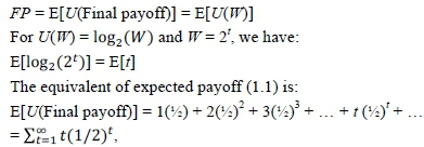
The equivalent of expected payoff (1.1) is:

 

5 Summary

Over the last 300 years, various analyses of, and solutions to, the St Petersburg Paradox have been offered. Applying the concept of discounted no-arbitrage pricing - based on the accepted model for obtaining fair prices for financial assets - to the St Petersburg Game shows that there is indeed no infinite price paradox. In this new framework, the price per game is finite, and there is a simple formula for pricing the game that depends on a discounting factor that can in theory be negotiated between bank and player. Finally: Although one may see the original St Petersburg Paradox as a case of a nonsensical question leading to a nonsensical answer, there is much to learn from the pricing exercise and the solutions to the "paradox".

 

References

BERNOULLI, D. 1738 (1954 translation). Exposition of a new theory on the measurement of risk. Econometrica, 22:23-36.         [ Links ]

BJÖRK, T. 2004. Arbitrage theory in continuous time. New York, US: Oxford University Press.         [ Links ]

BOREL, E. 1949. Le paradoxe de Saint-Pétersbourg. C.R. Acad. Sci. Paris, 228:404-405.         [ Links ]

BRU, B., BRU, M.-F. & CHUNG, K.L. 2009. Borel and the St Petersburg Martingale. Electronic Journal for the History of Probability and Statistics, 5(1):1-58. Available at: www.jehps.net [accessed June 2014].         [ Links ]

BUFFON, G.L.L. 1777. Essai d'arithmétique morale. Supplement l'Historie Naturelle, vol. IV.         [ Links ]

DURRETT, R. 1996. Probability: Theory and examples. California, USA: Duxbury Press.         [ Links ]

FELLER, W. 1945. Note on the law of large numbers and "fair" games. Annals of Mathematical Statistics, 16(3):301-304.         [ Links ]

FELLER, W. 1968. An introduction to probability theory and its applications. New York USA: John Wiley & Sons.         [ Links ]

MACKINNON, N. 1990. A lesson on the St Petersburg paradox. The Mathematical Gazette, 74:51-53.         [ Links ]

MAZLIAK, L. & SHAFER, G. 2009. The splendours and miseries of martingales. Electronic Journal for the History of Probability and Statistics, 5(1): Introduction. Available at: www.jehps.net [accessed June 2014].         [ Links ]

MENGER, K. 1934. Das Unsicherheitsmoment in der Weltlehre. Z. Nationalökon, 51:459-485.         [ Links ]

PLISKA, S.R. 1997. Introduction to mathematical finance. Oxford, UK: Blackwell Publishers.         [ Links ]

SAMUELSON, P.A. 1977. St Petersburg paradoxes: Defanged, dissected, and historically described. Journal of Economic Literature, 15(1):24-55.         [ Links ]

VIVIAN, R.W. 2013. Ending the myth of the St Petersburg paradox. SAJEMS NS, 16(3):347-364.         [ Links ]

 

 

Accepted: February 2016