ARTICLES

 

Trading book risk metrics: A South African perspective

 

 

Dirk Visser^I; Gary van Vuuren^II

^ISchool of Economics, Department of Risk Management, North-West University & NedBank, South Africa
^IISchool of Economics, Department of Risk Management, North-West University & Aviva Investors, UK

 

 

---

ABSTRACT

The regulatory market risk metric - Value at Risk - has remained virtually unchanged since its introduction by JP Morgan in 1996. Many prominent examples of market risk underestimation have undermined the credibility of VaR, prompting the search for better, more robust measures. Expected shortfall and procyclical capital buffers have been proposed by regulatory authorities, but neither is without problems. Bubble VaR -a coherent measure which avoids many of the pitfalls to which other measures have succumbed - was designed to be both forward-looking and countercyclical. Although tested on other markets, here it is applied to various South African prices and the results compared with both international observations and other market risk measures. Bubble VaR is found to perform consistently and reliably under all market conditions.

Key words: value at risk, bubble VaR, expected shortfall, procyclical, trading book

---

 

 

1 Introduction

The regulatory market risk metric - Value at Risk (VaR) - was introduced by JP Morgan's RiskMetrics in 1994 (JP Morgan, 1996) and later popularised by the Basel Committee for Banking Supervision's (BCBS) 1996 amendment to the Basel I accord (BCBS, 1996). The revision encouraged qualifying banks to use internal models - invariably a VaR variant- if sufficient sophistication had been demonstrated to use the BCBS's internal models approach for market risk in the trading book. A standardised approach (a stylised, formulaic methodology which employed supervisory-determined parameters) was permitted (by the BCBS) for banks with no internal or poorly-performing models. In essence, the VaR methodology determines the possible loss on a current portfolio of securities over a specified time frame with a given probability. The method revalues the portfolio to establish potential losses under different scenarios (historical, simulated or those selected from a prescribed profit and loss distribution).

After the 2007/8 credit crisis, the G20 demanded that the BCBS improve regulations governing bank capital (G20, 2009). This was a complex task, requiring not only considerable improvements, but also substantial re-design of large parts of the entire regulatory framework. In response, the BCBS introduced an assortment of regulatory capital revisions in July 2009 to address failings exposed by the credit crisis (BCBS, 2009). Known collectively as Basel 2.5, these rules were primarily designed to reduce procyclicality of the market risk framework by adding a stressed VaR (in which the current portfolio is re-valued under severe market shock scenarios - SvaR) to the current VaR. Under the Basel II accord, although counterparty default risk and credit migration risk were addressed, mark-to-market (MTM) losses due to credit valuation adjustments (CVA) were omitted. Since two-thirds of losses attributed to counterparty credit risk during the credit crisis were due to CVA losses (with one-third due to actual defaults), an incremental risk charge was introduced to address default risk and credit migration in the trading book (BCBS, 2011a).

The new rules also harmonised the treatment of securitisation exposures across banking and trading books.

Further regulatory amendments were established with the issue of the Basel III rules in December 2010 (BCBS, 2011a). These introduced a countercyclical capital buffer (designed to increase capital requirements in boom times and release capital in downturns), instituted two liquidity risk measures (the shorter term Liquidity Coverage Ratio and the longer term Net Stable Funding Ratio), established a Pillar 1 leverage ratio, incrementally improved the quality and quantity of qualifying capital and augmented the regulatory treatment of market risk in the trading book via three specific provisions: (i) a capital requirement to protect against changes in counterparty creditworthiness (and associated MTM losses), (ii) a direct influence of unrealised MTM gains and losses on Tier 1 capital, and (iii) the exclusion of Tier 3 capital as eligible capital for market risk regulatory capital requirements.

Despite the modifications and amendments to the regulatory treatment of the trading book, several deficiencies in the internal models approach were noted:

1) VaR informs nothing about loss severity, only loss probability. This feature has long been a criticism of VaR yet despite this (and other factors) VaR's prominence in the regulatory framework has remained virtually unchanged since its introduction in 1996 (Duffie & Pan, 1997; Balbas, Garrido & Mayoral, 2009);

2) some capital charges overlap and are occasionally duplicated (e.g. SVaR/current VaR) (Coste, Douhady & Zovko, 2011; Choudhry, 2013);

3) the boundary between the trading book and banking book remains confusing (interest rate risk is only capitalised in the trading book, not the banking book (Yeh, Twaddle & Frith, 2005)) and vulnerable (the treatment of securitisation products between banking and trading books is inconsistent (Bank of England, 2014)); and

4) the measurement of market illiquidity is inconsistent and inadequately captured (the liquidity horizon or holding period is capped at 10 trading days, even though this was demonstrably insufficient during the credit crisis (International Monetary Fund, 2008)).

The standardised approach fared little better than the internal models approach. It had been shown to be risk-insensitive, inadequately capturing risks associated with complex instruments and dealing with hedging and diversification ineffectively (Prescott, 1997; Penza & Bansal, 2001).

The BCBS acknowledged that the incremental changes introduced by Basel 2.5 were both temporary and insufficient, and that a detailed review of mistakes made (and ways to repair them) was required. The fundamental review of the trading book, a substantially-revised market risk framework, was a direct result of that enterprise (BCBS, 2013). To strengthen capital standards for market risks, the BCBS proposed six sweeping changes to the measurement and management of trading book risks in a recent consultative document (BCBS, 2013). Figure 1 provides a summary of the framework constituents.

 

 

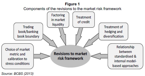
Although the proposals cover several facets of the trading book, banks' market risk capital will be most affected by four significant changes (BCBS, 2013):

1) VaR will be replaced as the desired market risk metric by expected shortfall (ES), the probability-weighted average of tail losses beyond a given VaR;

2) the VaR confidence level will be reduced from 99.0 per cent to 97.5 per cent;

3) expected shortfall (ES) will be scaled using stressed observations (thereby reducing the double-counting introduced by SVaR); and

4) holding periods will be asset-dependent and calculated using overlapping windows (no longer just 10 days for all trading book assets).

Prior to the 2013 BCBS proposals, Wong (2011) suggested a novel risk measure - bubble VaR (buVaR) - to address problems associated with market risk measures. Wong (2011) demonstrated that buVaR could transform VaR into a countercyclical measure, account for large tail losses and distinguish between long and short positions by modelling all portfolio return components simultaneously (unlike VaR which models only noise). Wong (2011) asserted that well-known VaR data requirements (such as portfolio return data stationarity and independent and identically distributed (i.i.d.) portfolio returns)may be relaxed using buVaR and empirical portfolio return observations, such as fat tails, high skewness and heteroskedasticty, could be included in the formulation. BuVaR generates supplemental buffers for these deviations from normality by only allowing crashes to occur counter to current market trends.

The suggestions put forward by the BCBS (2013) and Wong (2011) are attempts to improve the regulatory market risk milieu and, although not contradictory, are quite different in their respective approaches. Claims of buVaR's superiority over traditional VaR are tested in a South African framework, by applying it to local market data. The results obtained are compared to current and proposed regulatory measures including some of the BCBS proposals (such as the procyclical buffer and the ES measure).

The remainder of this article proceeds as follows: Section 2 explores problems with current and proposed regulatory measures including the non-subadditivity of VaR, issues with liquidity scaling, the omission of procyclicality from the market risk formulation and time-varying volatility issues. Section 3 explains the reasoning behind Wong's (2011) buVaR concept and details how the measure may alleviate many regulatory issues with current and proposed metrics. The data used to explore differences between the metrics are explained in Section 4, as well as all relevant mathematics. The results obtained from an analysis of South African data using various market risk metrics follows in Section 5 and Section 6 concludes.

 

2 Problems with regulatory market risk measures

2.1 Choice of market metric

VaR does not capture the tail risk of loss distributions (Rosenberg & Schuermann, 2004), and thus a conditional measure (i.e. given that a VaR threshold has been exceeded, what is the severity of the resulting losses?) is required. ES refers to the probability-weighted losses (thereby accounting for both loss severity and likelihood) in the tail beyond VaR (Nadarajah, Zhang & Chan, 2013).

A common criticism of VaR is that it employs historical data and therefore is of limited use for predicting uncertain futures, but the same is also true of ES. The Basel proposals (BCBS, 2013) stipulate that both the internal models-based approach capital requirements as well as the risk weights for the revised standardised approach must be determined using ES.

The BCBS has proposed a new VaR confidence level of 97.5 per cent (current: 99 per cent), so the ES will measure probability-weighted losses beyond this threshold. This new confidence level provides a similar risk level as the existing 99 per cent VaR threshold (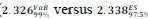 - a 0.5 per cent difference for the normal distribution) as shown in Figure 2. With more observations in the 2.5 per cent tail (compared with the previous 1 per cent tail), the move to ES is expected to

 

 

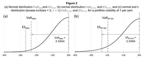
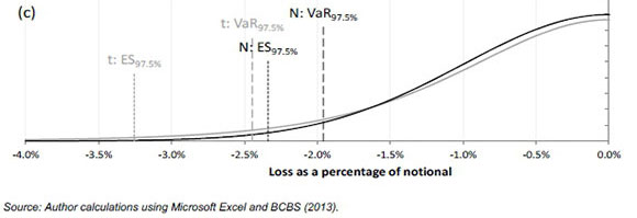
provide more stable model output and reduce sensitivity to extreme outlier observations. Banks may choose to use fatter-tailed distributions: Figure 2(c) indicates the difference between normal distribution and t-distributed assumptions.

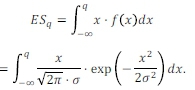
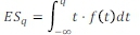
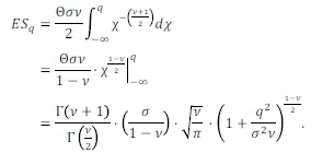
The expected shortfall at a certain quantile, q, is ES_q, the probability weighted average of values in the tail of the distribution to the left of q such that:

i.e. the probability density of the normal distribution, where a_tis the volatility, f(x) denotes the probability density function of JV(0, σ²) and it has been assumed that μ = 0.

To calculate ES_qfor any volatility, σ, and at any significance level, q, the function below must be integrated:

Let

Substituting

For other distributions, say the _t-distribution, which has fat-tails and is occasionally considered a better representation of VaR, integrate:

In this case, f (t) is the probability density function of the t-distribution which is (for μ = 0 and standard deviation, ):

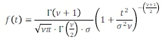
Where ν counts the degrees of freedom, calculated using:

and where k is the kurtosis of the data (Rozga & Americ, 2009).

To calculate ES_qfor any volatility, σ, any number of degrees of freedom, v, and any significance level, q, the integral below must be determined:

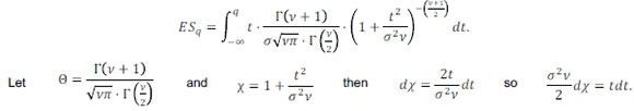
Substituting

Advanced simulation and sampling techniques are needed for ES tail event measurements: these require orders of magnitude more simulation scenarios so banks will find it considerably more difficult to back test ES (that considers both loss size and likelihood) than VaR (that only considers loss likelihood) (Yamai & Yoshiba, 2002). For VaR, violations are observable variables, facilitating the application of formal statistical procedures to determine if the distribution of the violations conforms to a (known) underlying model, i.e. model predictions are compared to observed outcomes. This is not true for ES model predictions as these may only be compared to model outcomes. Despite the variety of procedures available for back testing ES, these are substantially inferior to the VaR equivalents (Nadarajah et al., 2013).

2.2 Scaling of liquidity horizon

Market illiquidity manifests itself in two ways: exogenously and endogenously. Exogenous liquidity refers to market-specific, average transaction costs and is taken into account using a "liquidity-adjusted VaR" approach (Diebold, Hickman, Inoue & Schuerman, 1998,), usually by scaling of short-horizon VaR to a longer time horizon with the commonly used square-root-of-time scaling rule. This method has, however, been found to be an inaccurate approximation in many studies (see, e.g. Diebold et al., 1998; Danielsson & Zigrand, 2006; Skoglund, Erdman & Chen, 2012) and it also ignores future changes in portfolio composition (Berkowitz & O'Brien, 2002).

Endogenous liquidity refers to the price impact of the liquidation of specific positions (Bervas, 2006). It becomes relevant for trades large enough to alter market prices and is characterised by the collective liquidation of positions, or when all market participants react similarly - giving rise to extreme liquidity risk. Costs associated with endogenous liquidity are not accounted for in the valuation of trading books, so attempts have been made to incorporate this risk in a VaR measure (Bervas, 2006). The time to liquidate positions depends on transaction costs, position size, trade execution strategy, and prevailing market conditions (Berkowitz & O'Brien, 2002). Current work suggests that endogenous liquidity risk could also be addressed by extending the VaR risk measurement horizon (see, e.g. Emna & Chokri, 2014; Dionne, Pacurar & Zhou, 2014).

2.3 Time varying volatility

Time-varying volatility and stochastic jumps in the data are features of many financial time series. The former can be effectively modelled using the exponentially weighted moving average (EWMA) technique or various versions of GARCH models (e.g. Galdi & Pereira, 2007; Tripathy & Gil-Alana, 2010). However, these techniques can still give rise to procyclical effects of VaR-based capital measures (Gabrielsen, Zagaglia, Kirchner & Liu, 2012). As time horizons lengthen, time-varying volatility also diminishes the accuracy of VaR measures.

Volatility estimates using stochastic jump models, in contrast, diminish the accuracy of longhorizon VaR measures (Eberlein, Kallsen & Kristen, 2003; Witzany, 2013). Distinguishing between time-varying volatility and volatility changes that owe to stochastic jump process realisations can be important for VaR measurement (Tasca & Battiston, 2012).

2.4 Backtesting

The BCBS requires VaR models to be regularly backtested as regulatory capital is assigned based upon the accuracy of the backtest results (BCS, 1996). Banks are required to demonstrate that all material trading book exposures are captured, and that the methodology implemented for the subsequent VaR calculation accurately (defined by the BCBS) estimates the likely maximum loss at a given confidence level.

The BCBS approach, however, exhibits limited power to control the probability of accepting an incorrect VaR model (Type 1 error) (Pena, Rivera & Ruiz-Mata, 2006). Unconditional backtests have also been shown to be inconsistent for backtesting historical simulation models (Escanciano & Pei, 2012). In addition, backtesting procedures that only focus on the number of VaR violations have been shown to be insufficient to determine the appropriateness of model assumptions (IARCP, 2012). No consensus has yet emerged on the relative benefits of using actual or hypothetical results (i.e. Profit and Loss (P&L)) to conduct backtesting exercises (IARCP, 2012).

2.5 Procyclicality

Several have criticised VaR-based capital requirements because of their procyclical nature (see, e.g. International Monetary Fund, 2007; Marcucci & Quagliariello, 2008; Youngman, 2009).

Capital rules based on VaR require lower capital in boom times and higher capital in downturns (BCBS, 2010), thereby inducing cyclical lending behaviour by banks, exacerbating the business cycle. No convincing solutions to how these concerns could be addressed in the regulatory framework have yet been offered (BCBS, 2011b). The BCBS proposed a solution in the form of a countercyclical capital buffer, which has the primary objective of protecting the banking sector against excess aggregate credit growth through an additional capital buffer (BCBS, 2010). The buffer attempts to reduce cyclical lending behaviour introduced by VaR-like models. To implement this metric the BCBS has suggested a one-sided Hodrick-Prescott (HP) filter to determine the long run trend of economic activity. Considerably varied results are obtained using the two different filters (Van Vuuren, 2012).

The long-term trend of aggregate credit growth normalised by real Gross Domestic Product (GDP) growth ratio is extracted using the one-sided HP filter. The countercyclical buffer is activated when the difference between the ratio and its long-term trend exceeds a specified amount. Thus if economic activity expands too rapidly the current ratio will exceed the long-term trend and trigger the buffer's implementation.

2.6 Systemic behaviour

When all banks follow a VaR-based capital rule, financial institutions may be incentivised to act in a similar way during economic up and downswings. This gives rise to endogenous instabilities in asset markets but these risks are not generally included in individual bank measures of trading book risks (BCBS, 2011b). This may also reinforce and strengthen existing procyclicality as similar actions may precipitate either a boom or a bust cycle.

2.7 Subadditivity

VaR has been criticised for lacking the property of subadditivity, i.e. compartmentalised, VaR-based risk measurements are not necessarily conservative (Artzner, Delbaen, Eber & Heath, 1999; Danielsson, Jorgensen, Sarma, Gennady & De Vries, 2005). Expected shortfall, which is subadditive (Acerbi &Tasche, 2002), continues to gain popularity among financial risk managers (Chen, 2014), yet faces criticism because of its relative complexity, computational burden, and backtesting issues (Yamai & Yoshiba, 2002).

Spectral risk measures (weighted average of outcomes in which bad outcomes attract larger weights) are a promising generalisation of expected shortfall. Like expected shortfall, spectral risk measures are coherent, but their results may also be related to risk aversion and utility functions through the weights given to the possible portfolio returns and as they exhibit favourable smoothness properties (Cotter & Dowd, 2006). Spectral risk measures require little additional computational effort if underlying risk models are simulation-based (Costanzino & Curran, 2014).

 

3 Alternative measures: Bubble VaR

Wong (2011) asserts that buVaR is based on the principle that financial variables are extremistan, thus precise measurements of tail risk are not achievable and that trading book measurements should only aim to become as accurate as possible. The purpose of buVaR is to make VaR more robust by rendering it countercyclical, i.e. able to act as a buffer against fat-tail losses, but also incorporate the benefits of ES. The metric accomplishes these aims by leading crashes and being able to distinguish between long and short positions.

VaR-like metrics and financial markets behave procyclically (BCBS, 2011a), but financial market participants also act in a manner which promotes this phenomenon. In times of financial proliferation institutions chase profitable positions and in recessions reduce their credit extensions to avoid declining volatile market positions. This amplifies the market cycle and, subsequently, procyclicality. To date (January 2015) the BCBS's best cure for this phenomenon has been the introduction of the countercyclical buffer (BCBS, 2011a). BuVaR may provide a sensible alternative as it accounts for the current cycle position and subsequently inflates either side of return distributions in an attempt to counter both the procyclical nature of VaR-like models (via inflated return distributions) and financial markets (via buffer increases).

Wong (2011) asserted that buVaR relaxes standard VaR assumptions including the stationarity and i.i.d. property of portfolio returns. Research has demonstrated that relaxing these assumptions compromises model tractability, estimation consistency and precision (Emna & Chokri, 2014; Escanciano & Pei, 2012), but Wong (2011) argues that these assumptions are regularly violated in any case during stressed market periods. In addition, if variables are extremistan (irreproducible and unpredictable) the assumptions of i.i.d. and stationarity may create an illusion of measurement precision of events that are inherently unpredictable (Wong, 2011). BuVaR requires that these assumptions be relaxed to glean the cyclical information present in price series (in contrast to return series). Using original prices relaxes the assumptions of i.i.d. and stationarity and can provide cyclical information, but may introduce the risk of increasing serial correlation in residuals leading to biased estimations.

Some problems associated with VaR may be explored by decomposing a price time series:

Xt = Lt + St + Zt(Et)

where the original price series, X_t, comprises the long-term trend, L_t, a cyclical component, S_tand a noise factor, Z_t. Z_tis derived by taking first differences and thus is the only component to be stationary and driven by an i.i.d. process. L_tand S_tcan be extracted using, for example, an HP filter or Fourier analysis. Conventional VaR, which uses portfolio returns only, deals with Z_tand thus loses valuable information embedded in the cyclical component, S_t. Wong (2011) suggests that crashes are only corrections of market cycles disturbed by bubbles. The introduction of buVaR penalises asset bubbles detected in S_tby inflating the portfolio return distribution in such a way that 'bubble chasing' is discouraged. Note that L_tis not penalised, so participation in real economic growth is not discouraged.

BuVaR has two essential properties that distinguish it from conventional VaR which collectively transform the original return distribution for calculation of regulatory capital in a forward-looking countercyclical manner. The ability of buVaR to detect the formation of market bubbles is made possible through the bubble indicator.

3.1 Bubble indicator

The bubble indicator, B_t, is defined in Section 4. For the moment, it suffices to know that it measures the formation of market bubbles (defined as the degree of price deviation from a series equilibrium level) and, in order to qualify as suitable, it must adhere to several requirements (Wong, 2011):

5) for a model to detect and respond to market procyclicality and introduce countercyclicality the indicator must be synchronised with - or ideally lead - the market;

6) the model must avoid bubbles, however, it should not penalise investments and growth by mistaking these for the possible onset of a bubble. Thus, the indicator must be able to differentiate between the initiation of an unsustainable bubble in S_tand sustainable long-term trends in L_t;

7) the indicator must be able to punish positions continuously that are against the crash (i.e. long positions in a dwindling market) throughout the entire crash. This should prevent institutions from entering these positions thereby exacerbating an already failing market. Institutions may look to over-expose themselves at favourable prices that the indicator attempts to limit, and

8) the indicator must be sufficiently stable to be used for estimating regulatory capital.

The bubble indicator must be constructed in such a way that if the bubble forms in an uptrend the bubble indicator triggers (inflating the negative side of the return distribution and vice versa):

 

Wong (2011) stresses that using a deviation of a price from its moving average (MA) as a bubble indicator will fail as it only satisfies the first property mentioned above. Figure 3 illustrates the calculation of B_tand a deviation from a simple MA respectively.

 

 

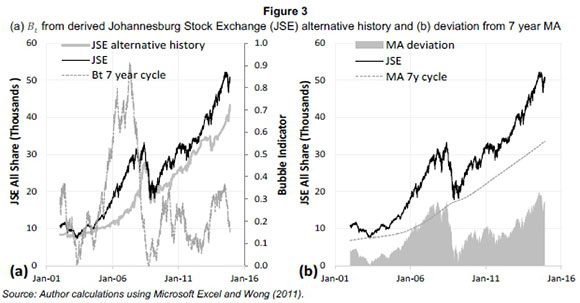
The B_tin Figure 3 a is smoother than the deviation from the seven year MA in Figure 3b making it more stable for the calculation of regulatory capital. The deviation from the MA behaves procyclically as it neither detects nor avoids bubbles.

3.2 Inflator

The second unique element of the buVaR metric is the inflator, calculated using a boundary argument. VaR is known to underestimate risk (Kourouma, Dupré, Sanfilippo & Taramasco, 2010), and thereby provides a lower boundary. A structural upper limit must also be determined: the inflator provides this upper limit as it increases in severity to ensure the avoidance of bubble formation during market stress. Wong (2011) suggests the inflator should also meet certain criteria to be deemed suitable. It should:

9) increase monotonically with the bubble indicator,

10) determine a structural upper limit which is logical and reasonable, but also sufficiently severe to prevent the manifestation of bubbles. A structural upper limit exists because of imposition of circuit breakers by regulators, and

11) not be generic, but should rather be adaptable to several assets as they have different characteristics. Wong (2011) refers to the "avoidance of a one-size-fits-all" multiplier.

The risk measure to calculate regulatory capital completes the buVaR model. Wong (2011) points out that ES is superior to conventional VaR because:

12) ES is subadditive and thus more coherent,

13) ES is relatively stable for the purpose of minimal regulatory capital estimations, ES seems to be suitably responsive to new market prices and regime switches and it aligns to suggestions and recommendations from the regulatory milieu.

In practice, the implementation and calculation of ES has been shown to be difficult (Taylor, 2008). ES is estimated conditional on VaR, giving rise to the possibility that estimation and model risk for ES will be higher than for VaR, although the smoothing of the tails implies ES could be more stable than VaR. Risk forecasts which use 97.5 per cent ES forecasts are more volatile than 99 per cent VaR forecasts. For example, for a Student-t (distribution), the 97.5 per cent ES is over 40 per cent more volatile than the 99 per cent VaR counterpart, while for the conditional normal it is more than 10 per cent higher (Danielsson, 2013).

The next section describes the data and methodology employed.

 

4 Data and methodology

4.1 Data

The data employed in the buVaR risk metric were daily closing prices for the following variables: JSE All Share Index, S&P500 Index, United States Dollar (USD) per South African Rand (ZAR) exchange rate, crude oil/barrel in ZAR and crude oil/barrel in USD. Weekly JSE All Share (ALSI) index data were also used for trend extractions. The period of the data spans January 1982 to January 2015. All calculations were performed in Microsoft® Excel®.

4.2 BuVaR calculation

1) The process to determine buVaR commences with the first differencing of the price series deriving returns for all previous days of n.

2) An inflator, A_t, is generated via rank filtering which is commonly used in digital signal processing. This process is used to remove the exceedances (outliers) from the price series and Wong (2011) found an 8 per cent filter applied to a 1000-day rolling window to be appropriate. The 1000-day (4 years' worth of trading days) window was found effective for US and Euro data as this period embraces at least one recent financial cycle. This may be adjusted accordingly depending on the data used as cycle lengths differ in markets and economies. Van Vuuren (2012) used Fourier analysis on the credit growth/GDP ratio (prescribed by the BCBS for determination of the countercyclical capital buffer) and found the South African market cycle to have a frequency of approximately seven years (see also Botha, 2009). Wong (2011) does, however, warn that ideally only one crisis (cycle-trough) at a time should be present in a window period as large amounts of volatile data could distort the window period.

3) Applying a rank filter of 8 per cent reduces R_n= 0 for all returns < 8% and > 92% quantiles for the rolling window {R_n,... R_n-1000} respectively. Wong (2011) sets the threshold for the rank filtering process at 8 per cent with the motivation that increasing it further would filter out too much information and subsequently flatten out bubbles and remove cyclical information. Reducing the bubble threshold would transform the method to a deviation from a simple MA which Wong (2011) showed to be ineffective.

4) The creation of growth factors for each n is accomplished using

D_n= exp(R_n)

5) An alternative history is then created, thus for each day, n, a 1000-day new price vector {P_n,..., P_n-1000} is created working backwards from X_nwith P_n= X_n.

 

In this alternative history, calculated growth was sustainable, gradual and market bubbles and manias did not occur.

6) Wong (2011) identifies the equilibrium μ_ηas the m-day MA of the alternative history created, where m is a non-constant expressed as:

 

Wong (2011) labels this as the adaptive MA and asserts that it has the effect of being able to reduce the bubble indicator (by reducing the window length m) when it detects that rallies conform more to long-term growth (L_t) than formation of assets bubbles. This is how the metric attempts not to penalise long-term growth but only the formation of assets bubbles.

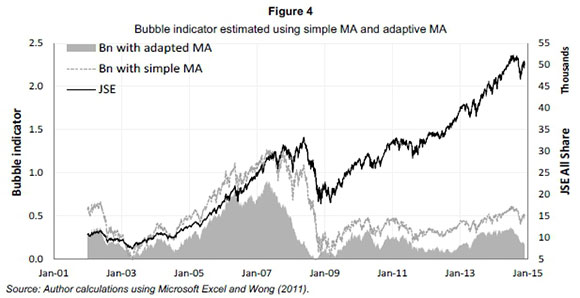
7) The bubble indicator is a simple construction defined as the price deviation from the equilibrium:

 

This metric is intended to measure the degree of cyclical bubble formation and unlike a simple MA it meets the criteria mentioned in Section 2 for a suitable bubble indicator. This advantage compared to a simple MA is shown in Figure 4 illustrating the bubble indicator estimated using a simple MA and Wong's (2011) suggested adaptive MA.

 

 

8) An inflator adhering to the criteria mentioned in Section 3 can be presented as:

 

ψ is (in absolute values) the average of the five largest losses and gains throughout the entire price history of the asset capped by a circuit-breaker, if applicable

B_maxis the largest absolute B_nobserved throughout the entire history of the asset

σ_t is the standard deviation of returns for the last 250 trading days and

w₂ = Changing response function.

Figure 5 illustrates a stress testing analysis of w₂in order to assess which level of w₂would provide the smoothest day-to-day variation of buVaR.

 

 

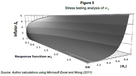
A w₂ = 0.5 [similar to Wong (2011)] was found to be the most workable estimate providing the smoothest variation of day-to-day buVaR.

The inflator acts as a multiplicative adjustment for every scenario, but only on the side of the return distribution of a 250-day observation period in line with the 12-month observation period for VaR as suggested by Basel II. As demonstrated in Section 3, the return distribution undergoes a transformation to the extent that if on day t:

14) B_t > 0,then all scenarios on the negative side should be multiplied by ∆_tin order to penalise long positions, but should be set to ∆_t= 1 for all positive returns

15) B_t < 0, then all scenarios on the positive side should be multiplied by ∆_tin order to penalise short positions, but should be set to ∆_t= 1 for all negative returns.

The buVaR metric, based on a historical approach evaluates a portfolio on shifted levels (X_i') which are based on a set of scenarios. To ensure that these shifted levels of the portfolio, asset or risk factor do not become negative they are calculated using log returns:

Where the scenario i = 1,2, ...,250 is the number days that have passed from day t and R_nis the original return series prior to applying the rank filter. Also η = t - i + 1. In this univariate case a bank's portfolio is first evaluated using a product pricing function g(.).Then for each scenario í the portfolio is evaluated at state X? to produce a value g(X[). The profit and loss (P&L) vector at day t is just the distribution of values [β(Χ[) - g(X_t)}, where g(X_i') is a 250-vector and g(X_t) a scalar. Let the sample distribution of this P&L be y. The buVaR at confidence level q per cent is the ES of the P&L distribution y estimated over a one day horizon at (1 - q) coverage:

BuVaR< = E(y\y < μ)

where:

Pr(y < μ) = 1 - q

The next section details the results obtained from various indices, commodity prices and exchange rates.

 

5 Results and discussion

BuVaR's two distinct features (the bubble indicator, B_tand the inflator, A_t) distinguish it from other market risk measurement tools. In addition, an essential element of buVaR is the use of an adaptive MA to calculate the growth factors, which in turn contributes to the estimations of B_tand ∆_t. Wong (2011) suggests and conducts buVaR using a four year window period in the adaptive MA, arguing that the data should not include more than one crisis period. However, a four year window period is not necessarily optimal for all economies and markets. Visual analysis, trend extraction and standard Fourier analysis are used in order to determine the most prominent cycle frequencies of the data used.

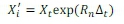
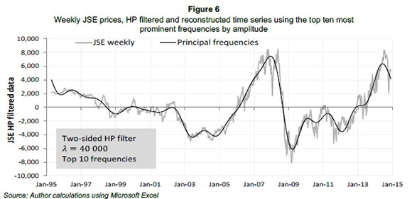
Figures 6 and 7 show weekly, HP-filtered prices for the ALSI and the S&P500 indices respectively, as well as the reconstructed time series using the top ten (by amplitude) cycle frequencies from Fourier analysis.

 

 

 

 

While the HP filter establishes and extracts the trend and results in a smooth series, the appropriate window period to use in buVaR must still be calculated.

The weekly price changes of the S&P500 (see Figure 7) show similar obvious downturns to those of the ALSI (see Figure 6), however, the effects of the internet bubble were very severe in the US market. This bubble's inception in 1997 saw several internet-based and related companies perform well, boosted by exceptional market confidence. However, the downturn caused several companies to close down as they had few tangible assets to absorb losses. The trend extracted in Figure 8 through visual inspection looks to show a frequency of between six and eight years, however this is not conclusive.

 

 

 

 

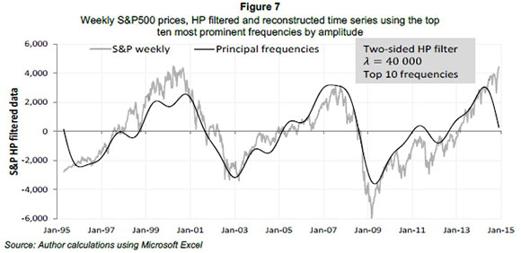
Standard Fourier analysis was used to extract cyclical market behaviour information and determine the relevant underlying frequency components. Results are shown in the frequency spectrum (Figure 8) for the ALSI and the S&P500. The frequency components for both time series indicate a principal frequency of approximately 6.8 years. The JSE has a secondary cycle of 4.1 years and the S&P 3.8 years.

The frequency amplitudes in Figure 8 shows that a seven year window period may account for a more prominent market cycle, making the adaptive MA more accurate by accounting for an entire cycle. The seven year window will also only account for one crisis at a time (avoiding the distortion of data) as the last three major crises occurred approximately 10 years apart (Wong, 2011). However, using a four year window period still has the possibility to yield noteworthy results as the frequency for this cycle length is still high and it makes it comparable to Wong's (2011) work.

The periodicity of market cycles and the amplitudes (prominence) of these cycles are affected in times of changing and volatile market conditions. The compression of market cycles is associated with increased serial correlation in the return series leading to volatility clustering (Wong, 2011). In stressed conditions cycle compression causes cycle lengths to shorten and the amplitudes of these shorter cycles to increase. The use of cycle compression in Figure 9 allows the analysis of cycle frequency amplitudes through different market conditions.

 

 

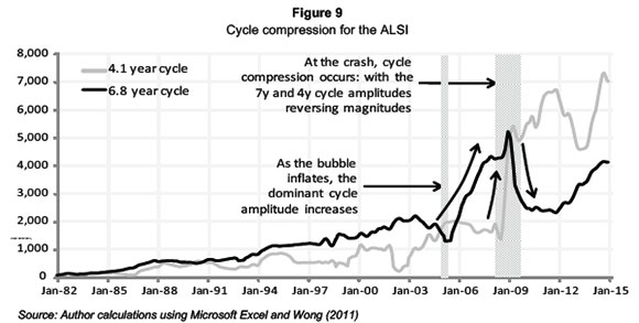
Figure 9 illustrates that the seven year cycle remains the prominent cycle for most of the analysis. From approximately 2005 the amplitude of the seven year cycle increases severely due to the prolonged market euphoria preceding the financial crisis (which began in Q3 2008). However, the onset of the crisis sees both series rapidly changing direction and the four year cycle amplitude becoming the prominent cycle. It is not unexpected for the shorter cycle length to increase in volatile, uncertain times. The cycle amplitudes converge again as stability returns to the market.

Figure 10 shows the application of buVaR on the ALSI from January 2002 until December 2014. Prior to January 2002 a seven year window period is used to apply the rank filtering process and subsequently create the alternative history where Wong (2011) suggests no market bubble or manias exist.

 

 

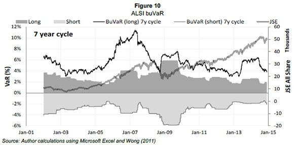
Figure 10 shows how the ALSI doubles in the two years commencing January 2004, however, buVaR and conventional ES move in opposite directions throughout this two year period. BuVaR peaks approximately a year before the market does and this highlights the countercyclical capabilities of the metric. The procyclical nature of conventional ES is illustrated in the periods from approximately January 2003 to January 2006, and January 2008 and January 2010, respectively. In the former period, the market increases gradually, but ES decreases due to the non-volatile favourable data being used to estimate ES.

BuVaR (through the bubble indicator and subsequent inflator) increases significantly, in an attempt to avoid the formation of a market bubble. In the latter period the market declines sharply with a significant increase in ES only followed three months later. The decline in buVaR after the financial crisis throughout the market rise is due to the metric avoiding the penalisation of long term growth.

The decline of buVaR before the onset of the crisis could be argued to be an underestimation of risk, however, the effect of the significant regulatory capital estimation by buVaR prior to the crisis may dissolve or avoid bubble formation. Wong (2011) asserts that due to buVaR leading crashes hindsight provides no benefit here. Statistical back-testing is not appropriate and hence visual testing has to be relied upon. BuVaR components for the seven year cycle estimations are shown in Figure 11.

 

 

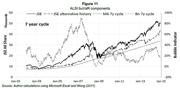
The significant increase in the bubble indicator in Figure 11 (used in the subsequent inflator) illustrates how buVaR attempts to identify potential market bubbles for penalisation. The bubble indicator is estimated from the JSE alternative history time series which in turn is estimated through the rank filtering process. The seven year MA of the original price series, which Wong (2011) asserts would not work as it does not conform to suitable characteristics for the estimation of the bubble indicator is also illustrated. The seven year cycle results are illustrated as estimations (Fourier analysis, HP filter and cycle compression) showing that the bubble indicator using this window period is more responsive. This is due to the more prominent seven year market cycle being accounted for, ensuring that the full boom and bust of the cycle are taken into account while not over-distorting the data and modifying them enough to get reputable results. The results produced by the four year cycle window period are also not flawed as this cycle was prominent throughout periods of increased volatility. However, for buVaR to be effective as a countercyclical risk measure it has to be consistently and continuously applied to a series in order to punish bubbles and prevent crises.

Figure 12 resembles Figure 11 with regards to buVaR peaking approximately a year before the onset of the financial crisis. The S&P500 suffered the financial crisis far worse than the ALSI as illustrated by their respective original price series in Figures 11 and 12. Similar to the JSE analysis conventional ES is late in crisis detection by almost an entire year. BuVaR shows spikes throughout the market euphoria from 2004 to 2008 possibly attempting to curb excessive growth in countercyclical manner. BuVaR peaks as volatility increases in the market in the latter part of 2007, however, the risk measure peaks again in the second half of 2009 and remains prominent for about three years. This may be due to the volatility of the market, but also the metric's countercyclical capability. This period in global finance is also highlighted by the sovereign credit crisis.

 

 

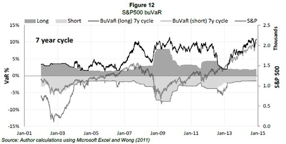
Noteworthy is the significant increase in buVaR from late 2013 up until January 2015, which may indicate the formation of a market bubble. In addition, several economists suggested that 2015 would be a good year for the global economy reinforced by the weak international oil price and the strengthening US economy (The World Bank, 2015; Mitchell, 2014).

The application of buVaR on the USD/ZAR exchange is illustrated in Figure 13.

 

 

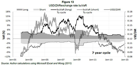
Applying buVaR to exchange rates may not only act as a warning signal to fluctuations, but may be used in conjunction with investments products affected by exchange rates. Between January 2002 and midway through 2004 buVaR produces similar results as conventional ES for the weakening rand. However, for all the periods or just before these periods where the rand experiences sharp declines, buVaR is elevated above conventional ES. The crisis period from 2008 to 2010 initially shows a significantly elevated buVaR with ES again being late in the detection of the severe decrease in the exchange rate. This reduction in the exchange rate may be due to investors divesting from emerging markets like South Africa. Also, in a challenging economic environment exports may drop possibly causing lower demand for the exchange rate as well. Figure 14 illustrates the application of buVaR on the price of crude oil per barrel in ZAR.

 

 

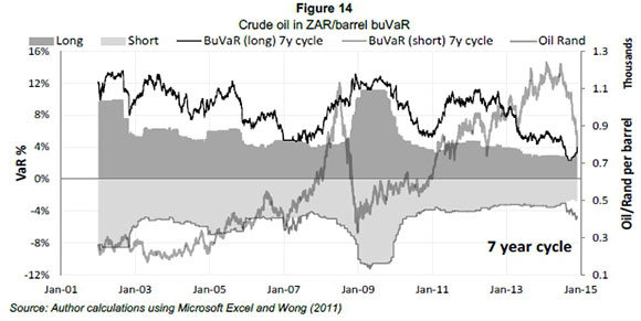
In Figure 14 buVaR diminishes as the price of oil increases gradually, however, when oil starts increasing significantly buVaR detects the bubble and changes direction whereas ES keeps decreasing. The spike in ES only occurs several months after the actual crash happens, thus emphasising the countercyclical ability of buVaR. BuVaR again swings upwards around 2011 and stays significantly elevated as the price of the commodity increases rapidly.

Oil peaks early in 2014 only to slump at the end of 2014 due to increased competition from the US and no decrease in supply from the Organisation of the Petroleum Exporting Countries (OPEC) (The World Bank, 2015). The depreciating ZAR is prominent in Figure 15, while constant increase in the price of oil from 2011 onwards is portrayed in Figure 14. In Figure 15, the price of crude oil in USD fluctuates, but on average remains flat for the same period.

 

 

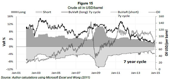
Figure 15 reflects similar results to those in Figure 14, with buVaR decreasing as the price of oil gradually increases. This aligns with the goal of buVaR not to punish growth, only bubbles. Again, buVaR increases as it detects the bubble whereas ES declines, only to increase sharply months after the severe decline in the oil price. BuVaR subsides quicker from 2011 onwards compared to Figure 14 where the depreciating ZAR - as depicted in Figure 13 - has an effect.

 

6 Conclusions and suggestions for future work

Relaxing the assumptions of i.i.d. and stationarity reduces the statistical estimation consistency and precision, but such assumptions are untrue when the market experiences stressed conditions anyway.

The BuVaR metric was demonstrated by Wong (2011) to be more accurate (rather than more precise) than VaR, providing a 'best guess' of losses. These values are situated somewhere between the VaR measured by traditional methods and a reasonable capped value. BuVaR does not generate a single solution for potential losses, but rather a practical value that may be effectively employed for determining risk capital. This value will be higher than a conventionally calculated VaR number, leading to a higher capital buffer, but compensates for the complex, fat-tailed loss distribution.

The financial crisis of 2008 emphasised the severe effects of behaviour, markets and risk metrics being procyclical in nature. This significantly underestimated phenomenon contributed to both the market euphoria and subsequent turmoil in global finance in the first decade of the 21^st century. The replacement of VaR by ES although an improvement on risk measurement, has not provided a solution in terms procyclicality. The BCBS has proposed the countercyclical capital buffer to be implemented January 2016 driven by the credit growth/GDP ratio (which has not been confirmed as the most suitable variable for all economies). However, the system wide implementation of countercyclical capital buffer may not be a straight forward process as all bank specific effects are still unidentified. For instance, banks in smaller or illiquid economies may struggle to implement minimum countercyclical regulatory requirements. Furthermore, what if one bank is an outlier in an economy and has to retain capital when it is in a downward slump or vice versa?

BuVaR provides a forward looking alternative to VaR attempting to account for procyclicality while incorporating the benefits of ES. Determining the appropriate length of market cycles is crucial in buVaR in order to calculate an effective alternative history. Fourier analysis and cycle compression provide adequate analysis of data in order to determine the length and prominence of market cycles. The analysis in Section 5 illustrates that buVaR detects bubbles and significantly increases required regulatory capital before ES does. This confirms the metric's countercyclical abilities to calculate regulatory capital in a forward looking manner.

Future research opportunities include the application of buVaR to considerably more portfolios, indices and commodities with different cycle characteristics. By observing output from many disparate sources, fat-tail loss patterns may be evaluated and connections established. The VaR measured under various market cycles (i.e. with distinct frequencies and amplitudes (severity)) differs from conventional VaR methods. Comparing these against buVaR estimates may provide some insight into the subtle interplay between market dynamics and portfolio or single asset losses.

Alternative histories may also be derived using different metrics, including the HP filter. The buVaR technique and the HP filter (for example) could be applied to relevant data and alternative histories constructed. The results obtained could be compared to establish differences and similarities and, with the benefit of hindsight, could lead research to the superior technique (since backtesting could easily establish which method produced the most accurate VaR estimates).

 

References

Acerbi, C. & Tasche, D. 2002. Expected shortfall: A natural coherent alternative to value at risk. Economic notes, 31(2):379-388.         [ Links ]

ARTZNER, P., DELBAEN, F., EBER, J. & HEATH, D. 1999. Coherent measures of risk. Mathematical Finance, 9(3):203-228.         [ Links ]

BALBAS, A., GARRIDO, B. & MAYORAL, S. 2009. Properties of distortion risk measures. Methodology and Computing in Applied Probability, 11(3):385-399.         [ Links ]

BANK OF ENGLAND. 2014. The case for a better functioning securitisation market in the European Union. Available at: https://www.ecb.europa.eu/pub/pdf/other/ecb-boe_case_better_functioning_securitisation_marketen.pdf [accessed November 2014].

BCBS. 1996. Amendment to the capital accord to incorporate market risks. Available at: http://www.bis.org/publ/bcbs24.pdf [accessed November 2014].

BCBS. 2009. Revisions to the Basel II market risk framework (updated 31 Dec 2010). Available at: http://www.bis.org/publ/bcbs148.pdf [accessed November 2014].

BCBS. 2010. Guidance for national authorities operating the countercyclical capital buffer. Available at: http://www.bisorg/publ/bcbs187.pdf [accessed November 2014].

BCBS. 2011a. Basel III: A global regulatory framework for more resilient banks and banking systems. Available at: http://www.bis.org/publ/bcbs189.pdf [accessed November 2014].         [ Links ]

BCBS. 2011b. Messages from the academic literature on risk measurement for the trading book. Available at: http://www.bis.org/publ/bcbs_wp19.pdf.         [ Links ] [accessed November 2014].

BCBS. 2013. Fundamental review of the trading book: A revised market risk framework (updated 31 Dec 2010). Available at: http://www.bis.org/publ/bcbs265.pdf [accessed November 2014].         [ Links ]

BERKOWITZ, J. & O'BRIEN, J. 2002. How accurate are value-at-risk models at commercial banks? The Journal of Finance, 57(3):1093-1111.         [ Links ]

BERVAS, A. 2006. Market liquidity and its incorporation into risk management, Banque de France. Financial Stability Review, 8(May):63-79.         [ Links ]

BOTHA, I. 2009. Modelling the business cycle of South Africa: Linear vs. non-linear methods, PhD thesis, University of Johannesburg. Available at: https://ujdigispace.uj.ac.za/bitstream/handle/10210/605/master.pdf?sequence=1 [accessed November 2014].         [ Links ]

CHEN, J. 2014. Coherence versus elicitability in measures of market risk. International Advances in Economic Research, 20(3):355-356.         [ Links ]

CHOUDHRY, M. 2013. An introduction to value-at-risk. (5^th ed.) Wiley: Chichester UK, 224p.         [ Links ]

COSTANZINO, N. & CURRAN, M. 2014. Backtesting general spectral risk measures with application to expected shortfall, working paper. Available at: http://papers.ssm.corn/sol3/papers.cfrn?abstract_id=2514403 [accessed November 2014]        [ Links ]

COSTE, C., DOUADY, R. & ZOVKO, I. 2011. The Stress VaR: A new concept or extreme risk and fund allocation. Journal of Alternative Investments, 13(3):10-23.         [ Links ]

COTTER, J. & DOWD, K. 2006. Extreme spectral risk measures: An application to futures clearing house margin requirements. Journal of Banking & Finance, 30(12):3469-3485.         [ Links ]

DANIELSSON, J. & ZIGRAND, J. 2006. On time-scaling of risk and the square-root-of-time rule. Journal of Banking & Finance, 30(10):2701-2713.         [ Links ]

DANIELSSON, J., JORGENSEN, B., SARMA, M., GENNADY, S & DE VRIES, C. 2005. Subadditivity re-examined: The case for value-at-risk. Discussion Paper 549. Financial Markets Group, London School of Economics and Political Science, London, UK.         [ Links ]

DANIELSSON, J. 2013. The new market risk regulations. VOX CEPR's policy portal. Available at: http://www.voxeu.org/article/new-market-risk-regulations [accessed January 2015].         [ Links ]

DIEBOLD, F., HICKMAN, A., INOUE, A. & SCHUERMANN, T. 1998. Converting 1-Day volatility to h-Day volatility: Scaling by Root-h is worse than you think, Wharton Financial Institutions Center, Working Paper 97-34. Published in condensed form as scale models. Risk, 11:104-107.         [ Links ]

DIONNE, G., PACURAR, M. & ZHOU, X. 2014. Liquidity-adjusted intraday value at risk modelling and risk management: An application to data from Deutsche Börse. Available at: http://ssrn.com/abstract=2398620 [accessed 02-11-2014]        [ Links ]

DUFFIE, D. & PAN, J. 1997 An overview of value at risk. The Journal of Derivatives, Spring, 4(3):7-49.         [ Links ]

EBERLEIN, E., KALLSEN, J. & KRISTEN, J. 2003. Risk management based on stochastic volatility. The Journal of Risk, 5(2):19-44.         [ Links ]

EMNA, R. & CHOKRI, M. 2014. Measuring liquidity risk in an emerging market: Liquidity adjusted value at risk approach for high frequency data. International Journal of Economics and Financial Issues, 4(1):40-53.         [ Links ]

ESCANCIANO, J. & PEI, P. 2012. Pitfalls in backtesting historical simulation VaR models. Journal of Banking & Finance, 36(8):2233-2244.         [ Links ]

G20. 2009. G20 Leaders Statement: The Pittsburgh summit. Available at: https://g20.org/wp-content/uploads/2014/12/Pittsburgh_Declaration_0.pdf [accessed November 2014].         [ Links ]

GABRIELSEN, A., ZAGAGLIA, P., KIRCHNER, A. & LIU, Z. 2012. Forecasting value-at-risk with time-varying variance, skewness and kurtosis in an exponential weighted moving average framework. Econometrics Journal, 12(1):82-104.         [ Links ]

GALDI, F. & PEREIRA, L. 2007. Value at risk using volatility forecasting models: EWMA, GARCH and stochastic volatility. Brazilian Business Review, 4(1):74-94.         [ Links ]

IARCP. (International Association of Risk and Compliance Professionals). 2012. 120 developments in risk management and compliance, ed. George Lekatis. Available at: http://www.risk-compliance-association.com/120_Developments_Risk_Management_Compliance_April_to_June_2012.html [accessed November 2014].         [ Links ]

INTERNATIONAL MONETARY FUND. 2007. Do market risk management techniques amplify systemic risks?" Global Financial Stability Report, October: 52-76.         [ Links ]

INTERNATIONAL MONETARY FUND. 2008. Market and funding illiquidity: When private risk becomes public. Global Financial Stability Report, April. Available at: https://www.imf.org/external/pubs/ft/gfsr/2008/01/pdf/sum3.pdf [accessed November 2014].         [ Links ]

JP MORGAN. 1996. Riskmetrics technical document. Available at: http://yats.free.fr/papers/td4e.pdf [accessed November 2014].

KOUROUMA, L., DUPRÉ, D., SANFILIPPO, G. & TARAMASCO, O. 2010.Extreme value at risk and expected shortfall during the financial crisis. Available at: http://dx.doi.org/10.2139/ssrn.1744091 [accessed November 2014].         [ Links ]

MARCUCCI, J. & QUAGLIARIELLO, M. 2008. Is bank portfolio riskiness procyclical? Evidence from Italy using a vector autoregression. Journal of International Financial Markets, Institutions and Money, 18(1): 46-63.         [ Links ]

MITCHELL, J. 2014. U.S. Job Openings hit 13-year high, The Wall Street Journal. Available at: http://blogs.wsj.com/economics/2014/08/12/rising-job-openings-quits-point-to-strengthening-labor-market/ [accessed January 2015].         [ Links ]

NADARAJAH, S., ZHANG, B. & CHAN, S. 2013. Estimation methods for expected shortfall. Quantitative Finance, 14(2):271-291.         [ Links ]

PENA, V., RIVERA, R. & RUIZ-MATA, J. 2006. Quality control of risk measure: Backtesting VaR models. The Journal of Risk, 9(2):39-54.         [ Links ]

PENZA, P. & BANSAL, V., 2001. Measuring market risk with value-at-risk. Financial Engineering Series, Wiley: New York, United States, 320p.         [ Links ]

PRESCOTT, E. 1997.The pre-commitment approach in a model of regulatory banking capital. Economic Quarterly, Federal Reserve Bank of Richmond, Virginia, United States.         [ Links ]

Rosenberg, J.V. & Schuermann, T. 2004. A general approach to integrated risk management with skewed, fat-tailed risks. Federal Reserve Bank of New York, Staff Reports no.185.         [ Links ]

ROZGA, A. & AMERICA, J. 2009. Dependence between volatility persistence, kurtosis and degrees of freedom. RevistaInvestigaciónOperacional, 30(1):32-39.         [ Links ]

SKOGLUND, J., ERDMAN, D. & CHEN, W. 2012. On the time scaling of value at risk with trading. Journal of Risk Model Validation, 5(4): 17-26.         [ Links ]

TASCA, P. & BATTISTON, S. 2012. Market procyclicality and systemic risk, ETH Risk Center - Working Paper Series, ETH-RC-12-012. Available at: http://web.sg.ethz.ch/ethz_risk_center_wps/pdf/ETH-RC-12-012.pdf [accessed November 2014].         [ Links ]

Taylor, J.W. 2008. Estimating value at risk and expected shortfall using expectiles. Journal of Financial Econometrics, 6:23-252.         [ Links ]

THE WORLD BANK. 2015. Global economic prospects. Available at: http://www.worldbank.org/content/dam/Worldbank/GEP/GEP2015a/pdfs/GEP15a_web_full.pdf [accessed January 2015].

TRIPATHY T. & GIL-ALANA, L. 2010. Suitability of volatility models for forecasting stock market returns: A study on the Indian national stock exchange, American Journal of Applied Sciences, 7(11): 1487-1494.         [ Links ]

VAN VUUREN, G. 2012. Basel III countercyclical capital rules: Implications for South Africa. South African Journal of Economic and Management Science, 15(3):309-324.         [ Links ]

WITZANY, J. 2013. Estimating correlation jumps and stochastic volatilities. Prague Economic Papers, 2(1): 251-283.         [ Links ]

WONG, M. 2011. Market buVaR: A countercyclical risk metric. Journal of Risk management in Financial Institutions, 4(4):419-432.         [ Links ]

YAMAI, Y. & YOSHIBA, T. 2002. On the validity of value-at-risk: Comparative analyses with expected shortfall. Monetary and Economic Studies, 20(1):57-85.         [ Links ]

YEH, A., TWADDLE, J. & FRITH, M. 2005. Basel II: A new capital framework. Reserve Bank of New Zealand Bulletin, 68(3):4-15.         [ Links ]

YOUNGMAN, P. 2009. Procyclicality and value at risk. Bank of Canada Financial System Review, June: 51-54.         [ Links ]

 

 

Accepted: August 2015