ARTICLES

 

Value-at-risk for the USD/ZAR exchange rate: The Variance-Gamma model

 

 

Lionel Establet Kemda^I; Chun-Kai Huang^II; Knowledge Chinhamu^III

^ISchool of Mathematics, Statistics and Computer Science, University of KwaZulu-Natal
^IIDepartment of Statistical Sciences, University of Cape Town
^IIISchool of Mathematics, Statistics and Computer Science, University of KwaZulu-Natal

 

 

---

ABSTRACT

A country's level of exchange risk is closely linked to its financial stability, on a macro-economic scale. South African exchange rates, in particular, have a significant impact on imports, inflation, consumer prices and monetary policies. Consequently, it is imperative for economists and investors to assess accurately the associated exchange risks. Exchange rates, like most financial time series, are leptokurtic and contradict the classical Gaussian assumption. We therefore introduce subclasses of the generalised hyperbolic distribution as alternative models and contrast these with the normal distribution. We conclude that the variance-gamma model is the most robust for describing the log-returns of daily USD/ZAR exchange rates and their related Value-at-Risk (VaR) estimates. The model selection methodologies utilised in our analyses include the robust Kolmogorov-Smirnov test and the Akaike information criterion. Backtesting on the adequacy of VaR estimates is also performed using the Kupiec likelihood ratio test.

Key words: South Africa, USD/ZAR exchange rate, Value-at-Risk, variance-gamma distribution, generalised hyperbolic distribution, robust Kolmogorov-Smirnov, Akaike, Kupiec

---

 

 

1 Introduction

"Exchange rate" can be defined as the value of a country's currency expressed in terms of another country's currency. The volatility and performance of a country's exchange rates are strongly related to its financial stability on a macro-economic scale. For example, Samson (2013) has observed that exchange rates have a significant impact on asset prices and firm values. Hence the focus on exchange rates has heightened in the wake of the recent financial crisis. In South African contexts, Aron, Farrell, Muellbauer and Sinclair (2014b) have shown that South African exchange rates are closely linked to import prices, inflation effects and market responses on monetary policies. Aron, Creamer, Muellbauer and Rankin (2014a) have also revealed that exchange risk is highly influential in South African consumer prices.

As a result, an accurate evaluation of risks associated with exchange rates is imperative for economists and investors. A common tool for risk assessments of financial variables, such as exchange rates, is the Value-at-Risk (VaR) measure. Some recent studies on the valuation of VaR for exchange rates include Zhou, Zhang and Chen (2013) and Batten, Kinateder and Wagner (2014).

The normality assumption of financial data was long denied by analysts such as Benoit Mandelbrot and Eugene F. Fama. Mandelbrot (1963) has shown that returns data display heavier tails than Pareto and Gaussian distributions. Similarly, Fama (1965) was able to show that the empirical distribution of daily prices on the Dow-Jones Industrial Average was more peaked in the centre, and had heavier tails, than the normal distribution. He further suggested the use of stable distributions. However, these distributions presented too heavy a tail to fit financial returns.

In the last two decades, a wide variety of econometric models have been suggested by researchers. For example, Hansen (1994) and Azzalini and Capitanio (2003), amongst other authors, proposed generalised skew /-type distributions for financial modelling. However, these models do not handle substantial skewness.

Barndorff-Nielsen (1977) introduced a family of continuous distributions, named the generalised hyperbolic distributions (GHDs), in which the logarithm of its probability density function is a hyperbola. Its first application was in the modelling of grain size distribution of windblown sand. These distributions proved to fit financial returns more adequately when compared to other distributions like the normal and student t distributions. For example, Eberlein and Keller (1995), using a data set consisting of daily prices of the 30 DAX over a period of three years, were able to show that GHDs presented the best fit to model data with a high frequency. Similar studies were carried out by Bibby and S0rensen (1996) and Prause (1999). Huang, Chinhamu, Huang and Hammujuddy (2014) also applied GHDs to model the South African Mining Index and to estimate its corresponding VaR values.

Other articles have also dealt with the application of GHDs to model exchange rates. For example, Aas and Haff (2006) showed that the logarithmic returns of the NOW/EUR (NOW is the Norwegian Krone) exchange rate has a heavier right tail than a left one, with the latter behaving more like the Gaussian distribution. Hence they proposed the use of generalised hyperbolic (GH) skew Student's t distribution and observed that it provides a better fit than the normal-inverse Gaussian distribution and the skew t distribution proposed by Azzalini and Capitanio (2003). Elsewhere, Fajardo, Farias and Ornelas (2005) used GHDs to model the USD/BRL (Brazilian Real) exchange rate and this produced more accurate VaR measurements than traditional approaches.

Another recent work on exchange rates and GHDs was carried out by Jowaheer and Ameerudden (2012). This research was mainly concerned with describing how the Mauritian rupee (MUR) varies along with the US dollar (USD) and the Indian rupee (INR), as they both play important roles in the Mauritian economy in terms of imports and exports. It is thus essential to model these exchange rates accurately. Jowaheer and Ameerudden found that the marginal distributions of MUR/USD and MUR/INR exchange rates were asymmetric and fat-tailed, following the hyperbolic distribution.

The various studies discussed above show that certain subclasses of GHDs provide suitable models for various financial data (in particular, certain exchange rates). However, limited studies have focused on identifying a suitable distribution and an adequate VaR model for South African exchange rates. Furthermore, it is not certain that previous studies would apply to the South African context. For instance, Vee, Gonpot and Sookia (2012) have suggested that the best models for different financial data may differ. Wong and Li (2010) have also shown that stock returns and exchange rates are negatively correlated, and that this correlation varies over different time periods.

The main contributions made by this article are as follows: firstly, we identify the variance-gamma (VG) distribution as the most suitable subclass of GHDs for describing daily USD/ZAR (ZAR is the South African rand) exchange rate log-returns, using statistical methods such as the robust Kolmogorov-Smirnov goodness-of-fit test and the Akaike information criterion. Secondly, we examine VG's adequacy in VaR estimation for the same data, relative to other GHD subclasses. Although VG has been utilised for modelling exchange rates (such as Tichý, 2006), it has been largely overlooked by the aforementioned studies. Moreover, it has not been used for VaR estimation in exchange rates and subsequently compared to other GHD subclasses. Thirdly, we discuss the rise of VG for modelling risks in the USD/ZAR exchange rate, as compared to models identified for other exchange rates.

The rest of the article is arranged as follows: in Section 2, we introduce the GHD family and its subclasses; Section 3 describes the statistical methodologies utilised for comparisons between different models; and Section 4 introduces the data and presents the corresponding descriptive analyses. Empirical results of the various statistical tests for model selection are presented and discussed in Section 5. Section 6 comprises the conclusion and offers suggestions for further research.

 

2 Generalised hyperbolic distributions

The generalised hyperbolic distribution is a five parameter continuous distribution. This distribution, together with its subclasses (namely, hyperbolic, normal-inverse Gaussian, VG and GH skew Student's t distributions), plays a significant role in the modelling of financial variables as it enables researchers to model data from a wide variety of fields such as economics and finance. This is mainly due to the fact that GHDs cater for asymmetry, heavy and semi-heavy tailed data. If a random variable X follows the generalised hyperbolic distribution, we write

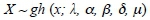
where μ is a location parameter, δ serves as a scaling factor, α determines the shape, β determines the skewness, and λ influences the kurtosis of the generalised hyperbolic distribution (Necula, 2009). Its probability density function is given by

where K_jis the modified Bessel function of the third kind, with order j. It should also be noted that the domain of the parameters must satisfy the following conditions

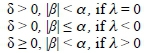
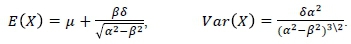
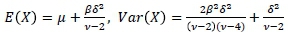
The mean and variance of this distribution (Prause, 1999) are given by

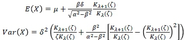
where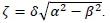

2.1 The normal inverse-Gaussian distribution (NIG)

This is a subclass of the generalised hyperbolic distribution obtained when the parameter λ = -0.5. Thus, a random variable X is said to follow a normal-inverse Gaussian distribution, denoted X ~ nig (x; α, β, δ, μ), if its probability density function is given by

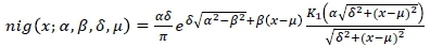
with x, μ ε |R and δ > 0, |β| < α. Also, for this distribution,

2.2 The hyperbolic distribution (HYP)

This is the subclass of GHDs obtained when the parameter λ = 1. Thus a random variable, X, is said to follow a hyperbolic distribution, denoted X ~ hyp (x; α, β, δ, μ), if its probability density function is given by

with x, μ ε |R. It should also be noted that different re-parameterisations of HYP exist. A particular case is given by

This parameterisation is very important in statistical analyses as it helps to determine the tail behaviour of the data. For instance, we have the following tail behaviours depending on the value of the parameter χ: if χ < 0, the left tail is heavier than the right tail, if χ < 0, the distribution is symmetric, and if χ < 0, the right tail is heavier than the left tail.

2.3 The variance-gamma distribution (VG)

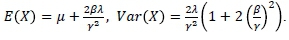
The third member of the GHD is obtained when the parameter δ -> 0. This subclass is called the VG distribution. A random variable following this distribution is denoted as X ~vg (x; λ, α, β, μ), and has probability density function defined by

where x ε R, Γ(λ) is the gamma function and γ ² = α² - β². The parameter domain is also given by λ > 0 and α > The mean and variance of this distribution are given by

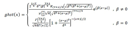
2.4 The generalised hyperbolic skew student's t distribution (GHST)

Finally, we have the GH skew Student's t distribution, which is the last subclass of the GHD family, and it is obtained as a limiting distribution when the parameters The probability density function of this distribution is given by

where we have used the fact that K_v(x) = . The mean and the variance of this distribution are given by

This distribution is the only subclass of the GHD with one polynomial and one exponential tail, thus enabling them to handle heavy-tailed data well.

 

3 Methodology

To test whether the subclasses of GHDs adequately describe our USD/ZAR exchange rate returns and to identify an optimal model, we utilise several statistical tests for model checking and selection. These are summarised below.

3.1 Robust Kolmogorov-Smirnov goodness-of-fit test

This test is closely related to the Anderson-Darling and Kolmogorov-Smirnov (K-S) tests for goodness-of-fit. But in this case, a "bootstrapping" procedure is performed. Our main reason for employing this test is because our sample size is large and the data contains many ties (i.e., repeated observations). The robust K-S test is useful in cases where the hypothesised distribution is not fully continuous (or discrete). More importantly, it also caters for data that contains ties, whereas the standard K-S test does not allow for ties in the data. The idea behind this test is to enlarge the region of acceptance hypothesis beyond that of the hypothesised distribution H(x), defined over some closed interval Z c |R. It should also be noted that this test is a two-sample test. The robust K-S test relies on the class of distributions defined by

where P(Z) is the space of all probability distribution functions on Z, and H and H~ are continuous probability distribution functions with nominal distribution H £ K. The hypotheses are, for some G ε K,

where D represent our data x1, x2, x3, . . . , xn. The test statistic is given by

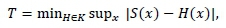
where S(x) denotes the empirical distribution of D, and is compared with some threshold value t. Thus, the null hypothesis, H₀, is rejected if T > t (Unnikrishnan, Meyn & Veeravalli, 2010).

3.2 Akaike information criterion (AIC)

Selecting the optimal model (i.e., the model that most accurately fits the data with minimum error) from a collection of models is a very important aspect in statistical analyses. Given that our analysis is principally based on fitting GHDs to data and comparing the fit of these distributions amongst one another for the optimal model, it is necessary for us to look at a criterion for model selection. In our case, we shall utilise the Akaike information criterion (AIC). This criterion suggests that the best possible model is the one with the smallest AIC value, with AIC given by

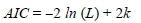
where k is the number of parameters in the model and L is the likelihood of the model.

3.3 Value-at-risk and backtesting

Value-at-Risk (VaR) is defined as a threshold value such that the probability of the market loss on a portfolio, over a given time horizon, exceeds this threshold value is equal to a pre-specified level. It is widely used as a risk measure and utilised for assessments of extreme behaviour in financial data (Jorion, 2006). More importantly, it can be used to measure a distribution's level of adequacy for tail fits, i.e. VaR backtesting.

It should be noted that financial institutions are more prone to failure due to the shortage of capital resulting from underestimation of VaR. Furthermore, Beling, Overstreet and Rajaratnam (2010) have shown that, under the Basel framework, there is a negative profit impact due to the misestimation of VaR in either direction. Hence, an adequate model for assessing the risk of a return series should not underestimate or overestimate VaR.

In the analysis of maximum loss for a portfolio, the Kupiec likelihood ratio test (Kupiec, 1995) is the most commonly used backtesting procedure. The Kupiec test relies on unconditional coverage, which means that it verifies whether the reported VaR estimate is violated significantly more, or a fewer number of times, compared to the level of significance, α. In this case, if the ratio of the number of violations is not significantly different from the level of significance, then the overall adequacy of the model is verified. Thus, under the null hypothesis that the ratio of the expected number of violations is a, the test statistic for the Kupiec test is given by

where Ν is the sample size and r" is the number of times the returns deflect below (for long position) or above (for short position) the estimated VaR value, at a level of significance. This test statistic asymptotically follows a chi-square distribution with one degree of freedom.

 

4. Data descriptives

As mentioned earlier, the data we consider in this research is the USD/ZAR exchange rate from the National Reserve Bank of South Africa. The data consists of the daily exchange rate from 04/01/1994 to 12/06/2015 and the values were collected daily at 10:30. No averaging or corrections were made to the data. In the following section, we introduce the data set and its descriptive analyses.

4.1 Time series plot

The time series of the daily USD/ZAR exchange rate is shown in Figure 1. It should be noted that the data consists of the weighted average of the banks' daily rates at approximately 10:30. Weights are based on the banks' foreign exchange transactions.

 

 

The first thing to note about this graph is that the daily exchange rate increased from about R3.40 per USD around 1994 to about R12.50 per USD around 2002, which is the highest it has ever reached since 1994. But as time went on, this value began to change haphazardly upwards and downwards to about R12.00 per USD in 2015. Thus the plot shows some irregular movements characterised by upward and downward trends. This suggests that the series is non-stationary. There is a very high degree of variability which is a common characteristic of financial data.

4.2 Descriptive statistics of log-returns of the daily USD/ZAR exchange rate

To transform the data to a stationary sequence, it is common practice to consider the log-return series (i.e., taking the first backward differences of the logarithm of the data values). Suppose our exchange rate data is given by the series {p₁, p₂, P₃, . . . , p_n}, where p_trepresents the exchange rate for day t. The log-returns (or just simply "returns"), at day t, of the series is given by

With this transformation, we obtain the time series plot and the corresponding histogram of the returns as shown below.

From the graphs below, we observe that the series hovers around zero, suggesting that the series is now stationary about the mean. However, we see some heteroscedastic patterns and volatility clustering, which characterise financial returns (Tsay, 2010). The histogram shows the leptokurtic behaviour of our log-returns as we have more returns at the centre than the tail parts, with a high peak around the mean, and fat tails.

 

 

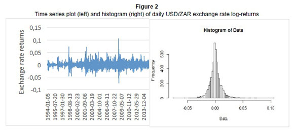
The leptokurtic behaviour is confirmed by Table 1 below, in which the kurtosis is as high as 9.423497. This also suggests that the log-return series is not Gaussian (as the kurtosis for normal distribution is 3). The Q-Q plot below also confirms this claim of non-normality; as normal distributed returns would imply that the returns lie in a straight line. Rather, our graph is S-shaped, which is due to the presence of fat tails, hence the need for heavy-tailed distributions such as the GHDs.

 

 

 

 

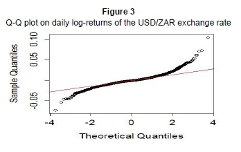
A formal test concerning normality is the Jarque-Bera normality test (also presented in Table 1). In our case, the test statistic has a value of 9548.103, with a p-value less than 0.00001, meaning that our null hypothesis of normality is rejected. The mean return of 0.0002417 also suggests a general increase in exchange rate since 1994. The skewness of 0.6060689 shows that the return series is not symmetric, as is commonly observed in financial data (Aas & Haff, 2006).

Figure 4 below shows the ACF plot of log-returns and that of squared log-returns for the USD/ZAR exchange rate.

 

 

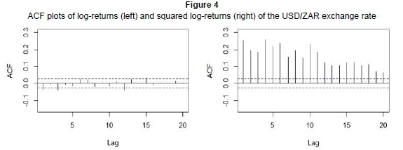
It is evident from the ACF plot of log-returns that our data are uncorrelated (all spikes are insignificant). However, the ACF plot of the squared returns shows some significant spikes, which suggests that the squared returns are autocorrelated. This is a common feature that characterises financial returns. These observations also confirm that the log-return series is stationary.

4.3 Test for stationarity

We perform two formal tests to confirm the stationarity of our return series; namely, the Augmented Dickey-Fuller (ADF) and the Philips-Perron (PP) unit root tests. Table 2 below summarises the results of both tests.

 

 

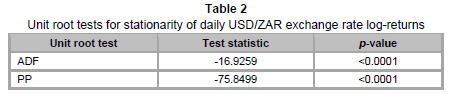
Under the null hypothesis of log-returns having a unit root, both tests show that this hypothesis is rejected at all levels of significance. This is indicated by the low p-values (both less than 0.0001). Hence our return series is stationary and we can proceed with further time series analyses.

 

5 Empirical results and model selection

This section focuses on the parameter estimation and comparison of fits for the subclasses of the GHDs and the normal distribution, on daily log-returns of the USD/ZAR exchange rate. Further, various tests are performed to select an optimal model for the USD/ZAR exchange rate's daily log-returns. We use the first 15 years of daily returns from 05/01/1994 to 02/01/2009 (3747 observations) for model training and in-sample testing, while the daily returns from 05/01/2009 to 12/06/2015 (1610 observations) are retained for out-of-sample testing.

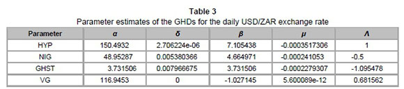
5.1 Parameters estimation for the GHDs

We estimate the parameters of the GHDs using maximum likelihood estimation (MLE). The table below illustrates the MLE parameter estimates for different subclasses of the GHDs.

Employing the estimates below, we proceed to analyse the goodness-of-fit for these GHDs and compare them to the normality assumption.

 

 

5.2 Comparison between GHDs and normal distribution

We begin with the comparison between the hyperbolic and normal distributions.

Figure 5 presents the various graphical analyses for the hyperbolic subclass. The histogram shows that the skewness of the hyperbolic distribution makes it more appropriate for fitting the daily log-returns, relative to the normal distribution. This observation is also made clearer by the log density plot, which is very important in the analysis of tail behaviour. In this case, it is evident that a heavy-tailed distribution such as the hyperbolic (with semi-heavy tail properties) is needed, as it provides a better fit compared to the normal distribution. This is further confirmed by the Q-Q plot, where it is evidenced that the hyperbolic distribution portrays a closer description of the data, especially at the tails.

 

 

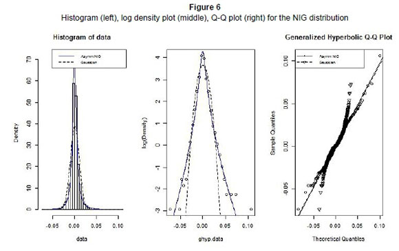
The graphs in Figure 6 illustrate the goodness-of-fit for NIG. Firstly, the histogram shows that NIG provides a better representation of the leptokurtic behaviour in daily log-returns of the USD/ZAR exchange rate. Secondly, the log density plot shows that the NIG distribution is more appropriate in fitting the tails, especially the upper tail of the log-returns and this is also finally, confirmed by the Q-Q plot. Thus once more, we obtain a better fit with NIG as compared to the normal distribution.

 

 

In a similar way to the above, we compare the fit of the normal distribution to that of GH skew Student's t distribution. The resultant graphical analyses are presented in Figure 7.

 

 

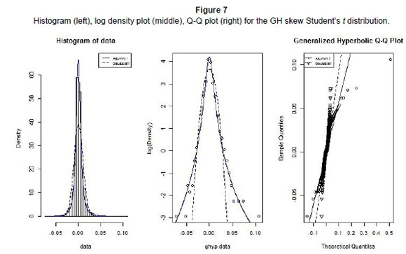
Relative to other members of GHDs, the plots in Figure 7 suggest that GHST provides the worst fit. However, relative to the normal distribution, it still shows a better depiction of our returns data, especially for the lower tail.

Finally, we compare the fit of the variance-gamma distribution to that of the normal distribution. In a similar way to the previous findings, Figure 8 shows that VG provides a better fit compared to the normal distribution as can be seen from the histogram and log density plot, in which the VG distribution fits the tails more accurately. Furthermore, the Q-Q plot shows that the VG distribution provides a very good fit to the lower tail.

 

 

In general, we have seen that the GHDs provide better fits for the daily USD/ZAR exchange rate log-returns than the classical Gaussian conjecture for financial data. The normal distribution deviates from the data most strikingly at the extreme tails, whereas the GHDs provide a more robust depiction of the tails. Concurrently, GHDs also cater for the skewness of our data set.

5.3 Goodness-of-fit test and model selection

As discussed earlier, the presence of ties and a large sample size motivates our use of the robust Kolmogorov-Smirnov (K-S) test. The table summarising the results of this test follows in the sequel.

 

 

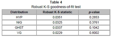
Through the "bootstrapping" procedure of the robust K-S test, we obtain the test statistics and p-values of the four GHD subclasses. Evidently, all subclasses demonstrate a high p-value, meaning we cannot reject the null hypothesis that the data follow these GHDs at all levels of significance. Furthermore, the robust K-S test shows that VG is the most robust of the four subclasses, with the lowest robust K-S distance and the highest p-value. Further comparisons may be drawn from a combined Q-Q plot of the subclasses against the data quantiles (see Figure 9).

 

 

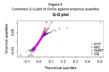
Clearly, the combined Q-Q plot suggests that NIG provides the best fit for the upper tail, while VG provides the best fit for the lower one. We may also observe that the GHST is, relatively speaking, the worst fit for both ends.

We now proceed to verify the selection of an optimal model using Akaike information criterion and log-likelihood values. These values will provide some insight into which subclass of GHDs is most robust for modelling our daily returns in general.

From Table 5, we observe that VG has the smallest AIC value of -24945.34 and the largest log-likelihood value of 12476.67. This means that the VG distribution provides the best fit compared to the other members. However, the differences between these AIC (and log-likelihood) values are diminutive. This is possibly as a result of all subclasses providing good depiction for the large bulk of data at the centre while their minor dissimilarities result from the varying tail fits of the distributions.

 

 

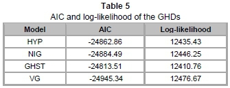
In financial terms, these tail behaviours relate to extreme risks. This has a major impact on the adequacy of capitalisation (e.g., for financial institutes) against such risks. Hence, to focus on these extreme tail fits, we utilise the Kupiec likelihood ratio test for comparing the number of violations to the corresponding Value-at-Risk level. We examine results from both in-sample backtests and out-of-sample tests. First, we take a look at the in-sample backtests.

Table 6 presents VaR estimates for different models at different levels of significance. In particular, the VaR values are estimated at 0.1 per cent, 0.5 per cent, 1 per cent, 99 per cent, 99.5 per cent and 99.9 per cent levels of significance.

 

 

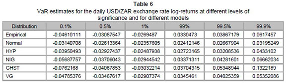
We observe that the VaR estimates from subclasses of GHDs are closer to those of the empirical distribution, compared to those of the normal distribution at almost all VaR levels. This was expected as we saw that GHDs provided a better fit compared to the normal distribution. In fact, the normal distribution underestimated VaR. On the other hand, GHST provided considerable overestimates for the upper tail, relative to the other models.

Table 7 represents the actual number of violations of VaR, as well as the expected number in brackets, at different VaR levels. These are utilised to obtain results for the Kupiec test. The p-values of the Kupiec test are summarised in Table 8 below.

 

 

 

 

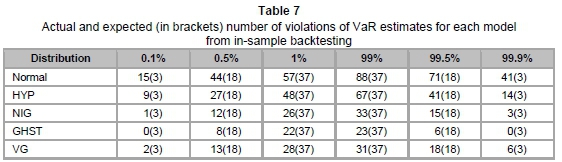
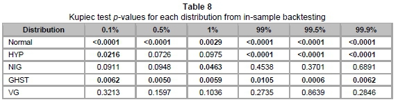
Table 8 above confirms the inaccuracy of the normal distribution for VaR estimation, where it is rejected by the Kupiec test at all VaR levels. This was anticipated, as it was earlier seen that the normal distribution provided an inadequate depiction of our data set. An interesting observation from the table is that NIG has high p-values at the upper tail (at 99 per cent, 99.5 per cent and 99.9 per cent) relative to the other subclasses of GHD. However, the lower tail is best fitted with VG, since it has the highest p-values at levels 0.1 per cent, 0.5 per cent and 1 per cent.

Overall, at the 5 per cent level of test significance, GHST is rejected at all VaR levels, HYP is rejected at four out of six VaR levels and NIG is rejected once. VG is the only model not rejected at any VaR levels at the 5 per cent level of test significance. Hence, we may select VG as the optimal model for the daily USD/ZAR exchange rate log-returns. Similarly, VG is the only model not rejected at all VaR levels at the 10 per cent level of test significance. In fact, at the latter level of test significance, all other models are rejected for losses, while NIG is the only other model not rejected for positive returns.

For out-of-sample testing, we forecast one-day-ahead VaR estimates by recalibrating the model parameters on a daily basis, using moving windows of the preceding 500 daily returns. The daily VaR estimates were calculated for the period from 05/01/2009 to 12/06/2015 (1610 observations) and compared with the corresponding realised daily returns. The resulting record of VaR violations is summarised in Table 9 and the corresponding Kupiec test p-values are presented in Table 10.

 

 

 

 

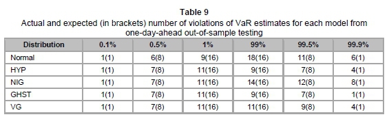
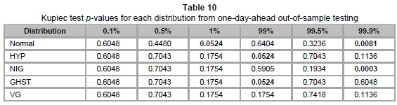
Due to the lack of data, as is common for out-of-sample testing, the results do not contrast as much as in the in-sample tests. In particular, no significant differences between the GHDs were observed for the lower tail, while Normal and HYP were the only models rejected once at the 5 per cent level of test significance. However, at the 10 per cent level of test significance, we again see that VG is the only model not rejected at all VaR levels. This further confirms VG as the most robust model for VaR estimation.

When comparing results from other research studies, we may also observe properties that are potentially distinctive to the USD/ZAR exchange rate. In particular, Aas and Haff (2006) have shown that VaR in the NOW/EUR exchange rate is well depicted by GHST, due to its dissimilar, heavy and semi-heavy, tails. However, in our analysis, GHST often produced overestimates for VaR in USD/ZAR and VG, with semi-heavy tails, producing more robust estimates. We suggest that this difference may be partially due to South Africa's prudent fiscal and monetary policies, meaning that the South African capital markets were not as largely affected by global financial crises as its international counterparts. At the same time, the USD/ZAR exchange rate is also correlated to the US market, which is one of the most commonly followed developed markets in the world. These resulted in the USD/ZAR exchange rate being uniquely different from other financial data, in that it is simultaneously affected by two vastly different markets.

 

6 Conclusion and further research

In this research we have provided assessments of the adequacy of generalised hyperbolic distributions (GHDs) for modelling the USD/ZAR exchange rate. In particular, our primary objective was to identify an optimal GHD subclass for depicting risks associated with the USD/ZAR exchange rate. Such a model should also capture stylised facts in financial data, such as skewness, asymmetry and heavy tails. Through various statistical analyses, we found that the generalised hyperbolic distributions provide better fits to the daily USD/ZAR exchange rate returns, than the classical Gaussian assumption. The robust Kolmogorov-Smirnov test and the Akaike information criterion both selected the variance-gamma distribution (VG) as the optimal model for the overall depiction of the daily USD/ZAR exchange rate returns. Furthermore, the overall Value-at-Risk (VaR) estimates produced from VG are the most robust, as suggested by the Kupiec likelihood ratio test, for both in-sample backtesting and out-of-sample tests. That is, VG does not significantly underestimate, nor does it overestimate, the expected number of VaR violations at all VaR levels under study. We also suggest that the distinct rise of VG for VaR estimation in the USD/ZAR exchange rate may be largely due to the fact that USD/ZAR is jointly correlated with two very different markets, the developed US market and the developing South African market, with vastly different structures and global focus.

Given that VG is the optimal GHD subclass to depict daily USD/ZAR exchange rate returns, further work could draw comparisons with the well-celebrated extreme value models, or incorporate VG into the framework of unconditional variance GARCH-based VaR models. Furthermore, multivariate GHDs and copula may be applied to study the dependencies among South African exchange rates and other financial variables, such as share prices, inflation rate and consumer indices.

R, Excel and SPSS were used to produce results of the various statistical tests and figures presented in this article.

 

References

AAS, K. & HAFF, D.H. 2006. The generalized hyperbolic skew Student's t-distribution. Journal of Financial Econometrics, 4(2):275-309.         [ Links ]

ARON, J., CREAMER, K., MUELLBAUER, J. & RANKIN, N. 2014a. Exchange rate pass-through to consumer prices in South Africa: Evidence from micro-data. The Journal of Development Studies, 50(1): 165-185.         [ Links ]

ARON, J., FARRELL, G., MUELLBAUER, J. & SINCLAIR, P. 2014b. Exchange rate pass-through to import prices, and monetary policy in South Africa. The Journal of Development Studies, 50(1):144-164.         [ Links ]

AZZALINI, A. & CAPITANIO, A. 2003. Distributions generated by perturbation of symmetry with emphasis on a multivariate skew t-distribution. Journal of the Royal Statistical Society B, 65(2):367-389.         [ Links ]

BARNDORFF-NIELSEN, O.E. 1977. Exponential decreasing distributions of the logarithm of particle size. Proceedings of the Royal Society London A, 353:401-419.         [ Links ]

BATTEN, J.A., KINATEDER, H. & WAGNER, N. 2014. Multifractality and value-at-risk forecasting of exchange rates. Physica A: Statistical Mechanics and its Applications, 401:71-81.         [ Links ]

BELING, P., OVERSTREET, G. & RAJARATNAM, K. 2010. Estimation error in regulatory capital requirements: Theoretical implications for consumer bank profitability. Journal of the Operational Research Society, 61:381-392.         [ Links ]

BIBBY, B.M. & S0RENSEN, M. 1996. A hyperbolic diffusion model for stock prices. Finance and Stochastics, 1(1): 25-41.         [ Links ]

EBERLEIN, E. & KELLER, U. 1995. Hyperbolic distributions in finance. Bernoulli, 1(3):281-299.         [ Links ]

FAJARDO, J., FARIAS, A. & ORNELAS, J.R.H. 2005. Analyzing the use of generalized hyperbolic distributions to value at risk calculations. Brazilian Journal of Applied Economics, 9(1):25-38.         [ Links ]

FAMA, E.F. 1965. The behavior of stock-market prices. Journal of Business, 38(1):34-105.         [ Links ]

HANSEN, B. 1994. Autoregressive conditional density estimation. International Economic Review, 35: 705-730.         [ Links ]

HUANG, C-K., CHINHAMU, K., HUANG, C-S. & HAMMUJUDDY, J. 2014. Generalized hyperbolic distributions and value-at-risk estimation for the South African mining index. International Business & Economics Research Journal, 13(2): 319-328.         [ Links ]

JORION, P. 2006. Value at risk: The new benchmark for managing financial risk (3^rd ed.) McGraw-Hill.         [ Links ]

JOWAHEER, V. & AMEERUDDEN, N.Z.B. 2012. Modelling the dependence structure of MUR/USD and MUR/INR exchange rates using copula. International Journal of Economics and Financial Issues, 2(1): 27-32.         [ Links ]

KUPIEC, P. 1995. Techniques for verifying the accuracy of risk measurement models. Journal of Derivatives, 2:173-184.         [ Links ]

MANDELBROT, B. 1963. The variation of certain speculative prices. Journal of Business, 36:394-419.         [ Links ]

NECULA, C. 2009. Modeling heavy-tailed stock index returns using the generalized hyperbolic distribution. Romanian Journal of Economic Forecasting, 2:118-131.         [ Links ]

PRAUSE, K. 1999. The generalized hyperbolic model: Estimation, financial derivatives and risk measures. Doctoral Thesis. University of Freiburg.         [ Links ]

SAMSON, L. 2013. Asset prices and exchange risk: Empirical evidence from Canada. Research in International Business and Finance, 28:35-44.         [ Links ]

TICHÝ, T. 2006. Foreign exchange rate modeling. Proceedings of Managing and Modelling of Financial Risks, 3:372-380.         [ Links ]

TSAY, R. S. 2010. Analysis of financial time series (3^rd ed.) Wiley & Sons, New Jersey.         [ Links ]

UNNIKRISHNAN, J., MEYN, S. & VEERAVALLI, V.V. 2010. On thresholds for robust goodness-of-fit tests. Presented at IEEE Information Theory Workshop, Dublin.         [ Links ]

VEE, D.N.C., GONPOT, P.N. & SOOKIA, N. 2012. Assessing the performance of generalized autoregressive conditional heteroskedasticity-based value-at-risk models: A case of frontier markets. Journal of Risk Model Validation, 6(4):95-111.         [ Links ]

WONG, D.K.T. & LI, K.-W. 2010. Comparing the performance of relative stock return differential and real exchange rate in two financial crises. Applied Financial Economics, 20(1-2):137-150.         [ Links ]

ZHOU, L., ZHANG, N. & CHEN, Q. 2013. Value-at-risk modelling for risk management of RMB exchange rate. International Journal of Applied Mathematics and Statistics, 43(13):297-304.         [ Links ]

 

 

Accepted: July 2015