


Services on Demand
Article
 English (pdf)
 Article in xml format
 Article references
Indicators

Related links
-
 Cited by Google
 -
 Similars in Google
Share

 Permalink
South African Journal of Economic and Management Sciences
On-line version ISSN 2222-3436
Print version ISSN 1015-8812
S. Afr. j. econ. manag. sci. vol.18 n.3 Pretoria 2015
ARTICLES
Measuring the impact of marginal tax rate reform on the revenue base of South Africa using a microsimulation tax model
Yolandé Jordaan; Niek Schoeman
Department of Economics, University of Pretoria
ABSTRACT
This paper is primarily concerned with the revenue and tax efficiency effects of adjustments to marginal tax rates on individual income as an instrument of possible tax reform. The hypothesis is that changes to marginal rates affect not only the revenue base, but also tax efficiency and the optimum level of taxes that supports economic growth. Using an optimal revenue-maximising rate (based on Laffer analysis), the elasticity of taxable income is derived with respect to marginal tax rates for each taxable-income category. These elasticities are then used to quantify the impact of changes in marginal rates on the revenue base and tax efficiency using a microsimulation (MS) tax model. In this first paper on the research results, much attention is paid to the structure of the model and the way in which the database has been compiled.
The model allows for the dissemination of individual taxpayers by income groups, gender, educational level, age group, etc. Simulations include a scenario with higher marginal rates which is also more progressive (as in the 1998/1999 fiscal year), in which case tax revenue increases but the increase is overshadowed by a more than proportional decrease in tax efficiency as measured by its deadweight loss. On the other hand, a lowering of marginal rates (to bring South Africa's marginal rates more in line with those of its peers) improves tax efficiency but also results in a substantial revenue loss. The estimated optimal individual tax to gross domestic product (GDP) ratio in order to maximise economic growth (6.7 per cent) shows a strong response to changes in marginal rates, and the results from this research indicate that a lowering of marginal rates would also move the actual ratio closer to its optimum level. Thus, the trade-off between revenue collected and tax efficiency should be carefully monitored when personal income tax reform is being considered.
Key words: microsimulation, tax efficiency, optimal tax, tax reform, personal income tax
1 Introduction
A vast body of literature exists arguing the features of an efficient tax regime and tax reform measures to improve on tax efficiency and collection. For example, Hassan and Bogetic (1996) find that collection is improved with a more simplified and efficient tax system with lower marginal rates and a broader tax base. According to Creedy (2010:140), a broad tax base with few exemptions and low tax rates serves as a "rule of thumb" for a good tax system. Bird (2008:12) finds that good tax policy in developing countries requires a tax system that minimises efficiency losses.
Adjusting personal income marginal tax rates and income bands is a powerful fiscal policy tool for government to affect the revenue base depending on the proportionality of the tax regime. Obviously, the secret is to adjust marginal tax rates until income is maximised and the negative impact on the economy is minimised. From a tax competition point of view, it is specifically useful to know how sensitive revenue is to the lowering of taxes, but also how tax efficiency responds to such changes. Feldstein (2011) shows that, in the United States, a combination of expanding the revenue base and reducing the marginal tax rates actually improves total personal income tax collection. Gwartney (2008:1) indicates that, from a supply-side perspective, relatively high marginal tax rates discourage productivity and encourage early retirement and even tax evasion.
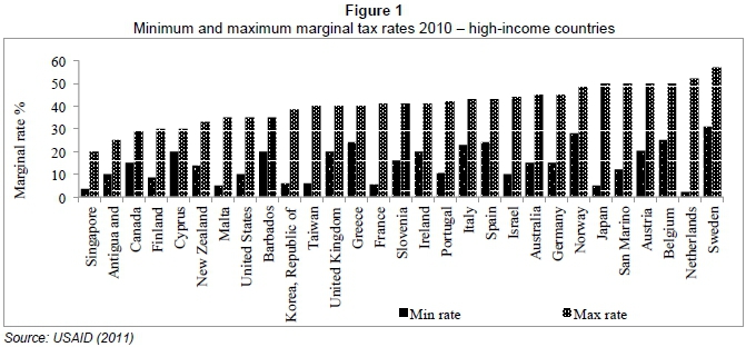
Tax reform over the past 30 years in the Organisation for Economic Co-operation and Development (OECD) countries was characterised by lower marginal tax rates and a reduction in the number of income brackets. However, it is important not to compare countries only by their marginal rates, but also to look at the threshold levels as well as the number of tax brackets (OECD, 2012:32). The empirical research of Peter, Buttrick and Duncan (2009:11) concludes that the average number of tax brackets for upper middle-, lower middle- and low-income countries should not exceed four to six brackets, thereby making the tax systems simpler to understand and to administer. It is suggested that the highest marginal rate for personal income tax (PIT) be set between 30 per cent and 50 per cent, and the lowest rate between 10 per cent and 20 per cent, with a few intermediate tax rates. The highest personal income group's marginal rate should be in line with the company tax rate to avoid tax arbitrage. If the highest PIT rate is lower than the company tax rate, companies will redistribute their profits to wages or give ownership of assets to individuals (Saunders, 2007).
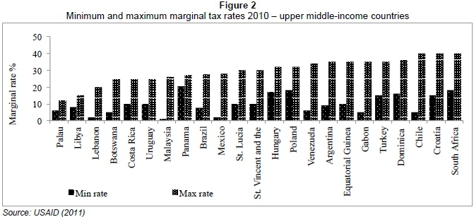
Figure 1 illustrates the maximum and minimum statutory marginal tax rates for 29 high-income countries in 2010 (United States Agency for International Development [USAID], 2011). The average minimum and maximum marginal rates are 15 and 40 per cent, respectively. Looking at 22 upper middle-income countries in Figure 2, the average minimum and maximum marginal rates are between 9 and 29 per cent, respectively (USAID, 2011).
Steenekamp (2012:50) compares marginal tax rates between South Africa and the Southern African Development Community (SADC) countries. He finds that South Africa's 40 per cent maximum marginal rate is higher than the 30 per cent average of SADC countries. A brief overview of the historic development of income tax reform in South Africa since the change in government in 1994 shows that the number of income bands was limited to nine and that individuals were taxed at a minimum and a maximum marginal rate of 17 and 43 per cent, respectively. At the time, they were also taxed differently on marital and gender status. In 1995/1996, only the highest marginal rate increased to 45 per cent, with the number of income bands stretched to 10, while gender differentiation was discontinued. In the 1997/1998 fiscal year, the lowest marginal rate increased to 19 per cent and the income bands decreased to seven. The tax-free threshold differentiated between individuals younger than 65 years and older than 65 years, while the child rebate was removed. In 1998/1999, the income bands were reduced to six, and, in 2000/2001, the top marginal rate decreased to 42 per cent, with a further reduction to 40 per cent in 2002/2003. From then onwards, South Africa's minimum and maximum marginal tax rates have remained on 18 and 40 per cent, respectively, which are substantially higher than the average for other upper middle-income countries (National Treasury, 2003).
In this paper, an attempt is made to identify the impact of an adjustment in marginal tax rates on revenue, efficiency and economic growth. A static microsimulation (MS) model is developed from survey data and used to simulate the proposed tax reforms. The choice of marginal-rate adjustments is based on international best practice with rates similar to those of South Africa's peers. The results show that such a lowering in rates to levels on a par with those of South Africa's peers has the potential to lead to improved levels of efficiency with the tax burden equal to, or even below, the optimal tax/GDP ratio from an economic-growth point of view. Although this ratio is below the optimal ratio, the results suggest that the loss in revenue could be minimised over time through a resultant increase in productivity and economic growth.
The structure of the rest of the paper is as follows: Section 2 explains the database and the adjustments that had to be made in order to bridge the gaps in published data, and the model results are validated against actual published South African Revenue Service (SARS) data. Section 3 explains the structure of the MS model. Section 4 validates the MS model results and Section 5 discusses the simulation exercises reflecting the impact of adjustments in marginal tax rates of individuals (upwards and downwards) on revenue, tax efficiency and economic growth. Section 6 concludes with some policy recommendations.
2 Data and methodology
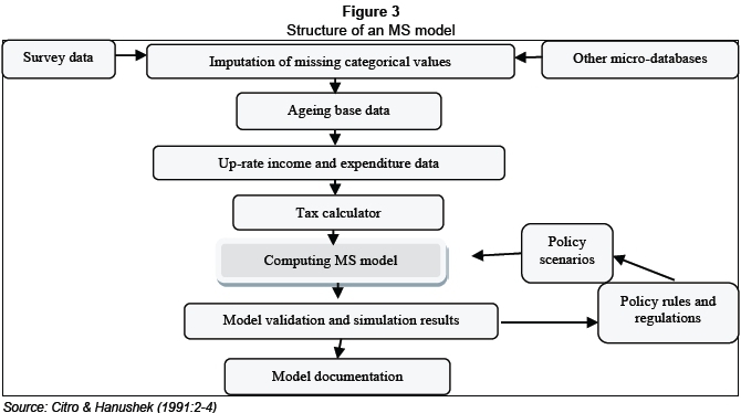
Data for MS tax models mainly originates from surveys with information on individuals' revenue collection and expenditure patterns. In the case of South Africa, the most representative survey is conducted by the Central Statistics Income and Expenditure Survey (IES), but, unfortunately, the information shows a high level of versatility (Statistics South Africa [Stats SA], 2008:1-2). Missing values as a result of non-responses due to refusal, unusable information and disqualified answers are common. In this paper, the 2005/2006 IES serves as the primary data set for the analysis. Income levels are calculated on an individual basis, with the profile of individuals explained by categorical variables such as gender, age group, education level, population group, and settlement. Some of the categorical information is unspecified, but these values cannot be excluded from the data set because the individuals are included in the weights of the survey and will affect the population total. To improve the data, the problem of unspecified values has been addressed through the imputation technique of Peichl and Schaefer (2009:3). The technique replaces unspecified values in each categorical group by the mean value of the specified values in the categorical groups. Figure 3 reflects the general structure of an MS model.
The gender variable differentiates between males and females and shows the extent to which each group is represented in the survey. Also, each individual in the household is categorised within a specific population group: African/black, Coloured, Indian/Asian, and white. Education groups range from no schooling, primary schooling, secondary schooling to degrees and diplomas. Only qualifications already obtained are included. Diplomas and certificates only count if at least six months of a course have been completed. Age is captured in completed years to the nearest completed number and is categorised in five-year age groups. Settlement is where the dwelling unit is located. Urban areas include cities and towns characterised by higher population densities, economic activity, and infrastructure. Rural areas include farms and traditional areas characterised by low population densities, economic activity, and infrastructure (Stats SA, 2008:1-2).
For the categorical variables in the IES survey containing unspecified data, a frequency table was obtained for each variable to determine the distribution of the unspecified values. When computing values for the unspecified categorical variables, the frequency distribution of the original responses remained unchanged. This methodology is available in the SAS program known as RANUNI (uniform random number generator). Briefly, the algorithm is as follows:
In equation 1, Rt is the ith random number, a is the multiplier and c the percentage increase.

The RANUNI function then generates a random number using a generator developed by Lehmer (1951) from a uniform (0, m) distribution, and turns it into (0,1) by dividing by ΓΠ. The number in parentheses is the seed/random number of the random number generator. If the seed is adjusted to a non-zero number, the same random numbers are being generated every time the program is activated (Fan, Felsövalyi & Keenan, 2002:26).
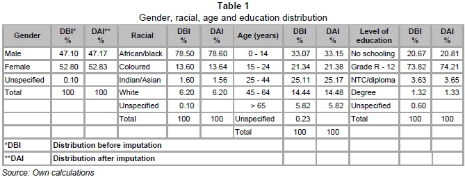
Table 1 shows that, prior to imputation, male responses account for 47.1 per cent and female responses for 52.8 per cent of the total, while non-responses amount to 0.1 per cent of the total population. Using the RANUNI statistical method, an unspecified value is replaced by a female response when the RANUNI is less than 52.8, or, alternatively, by a male response should the RANUNI be less than 47.1 per cent. It is evident that the female and male distribution before and after the imputation has only deviated slightly between males and females. After imputation, the male ratio only increased from 47.1 to 47.17 per cent and the female ratio from 52.8 per cent to 52.83 per cent.
In Table 1, the racial distribution before imputation is as follows: Africans account for 78.5 per cent, Coloureds for 13.6 per cent, Indians/Asians for 1.6 per cent and whites for 6.2 per cent of the total population. The non-response number amounts to 0.1 per cent for the total population in the survey. After imputation, the distribution between the racial groups only changes marginally. For example, the ratio for African/black only increases from 78.5 to 78.6 per cent.
Table 1 shows that, before imputation, the age group 0 to 14 years accounts for 33 per cent of the population. For age group 15 to 24 years, 25 to 44 years, 45 to 64 years, and 65 years and older, the distribution is 21.3, 25.1, 14.5 and 5.8, respectively. The non-response number amounts to 0.23 per cent. Again, the age group distribution after imputation only adjusts marginally. For example, the age group 15 to 24 years increases from 21.34 to 21.38 per cent, while the age group 65 years and older increases from 5.81 to 5.82 per cent.
The distribution of the education categories before and after imputation can be seen in Table 1. The group with no schooling represents 20.7 per cent of the population. Those with primary and secondary schooling (Grade R to Grade 12) represent 73.8 per cent of the population, while those with a national diploma only represent 3.6 per cent and those with a degree only 1.3 per cent. After imputation, the distribution between the education groups only changes marginally. For example, the share of the group with no schooling increases from 20.7 to 20.8 per cent, while those with school education increases from 73.8 to 74.2 per cent.
To validate the MS database against the 2005/2006 SARS filer data (Tax Statistics, 2010), a problem with different base years (calendar versus fiscal year) was encountered. Given the fact that the MS model is a tax model, the calendar year survey data had to be recalculated to fiscal years. The IES data has also been reweighted to take account of the population change for the fiscal year 2005/2006. The method used is the CALMAR reweighting program (Sautory, 1993), which recalculates the weights according to control totals, gender, race, and age group in order to match the population totals produced by Stats SA. The population total of the 2005/2006 IES equals the Stats SA midyear population survey of 2006 (Stats SA, 2005). Therefore, the 2005 midyear population survey is used with the 2006 midyear survey to rework the numbers to the fiscal year 2005/2006. The CALMAR method is also used by Stats SA and the modellers of the EUROMOD (Immervoll & O'Donoghue, 2009:2) and SAMOD (Ntsongwana, Wright & Noble, 2010:2) models.
3 Structure of the model
The approach followed is to construct an MS tax model - a technique used internationally for the empirical analysis of the effect of fiscal policy changes on revenue collection and expenditure, especially health care and retirement as well as other socio-economic expenditures (Buddelmeyer, Creedy & Kalb, 2007:3). It also allows for individual characteristics such as the composition of the taxpaying population in terms of age, gender, income levels, etc., and is especially useful to simulate individual income and expenditure behaviour as a result of policy changes that affect revenue (Citro & Hanushek, 1991:15). This is in contrast to macro-models which are structured on an aggregate level without the detailed information of individuals/households captured in the micro-model (Štěpánková, 2002:36). The model is a static one in which demographic characteristics are not aged.
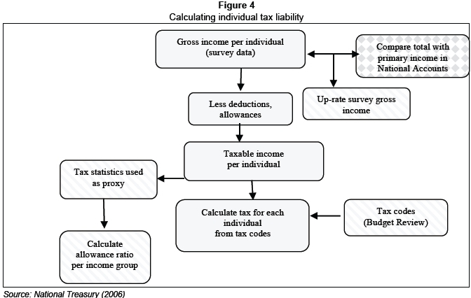
Figure 4 illustrates how individual tax liability is calculated. Total gross income of individuals (R749 billion) is compared with gross primary income (Rl 014 billion1) in the production, distribution and accumulation accounts of South Africa (South African Reserve Bank [SARB], 2012). Primary income is adjusted to the fiscal year 2005/2006 and excludes business income of about 7 per cent in order to account only for households. A factor of 1.352 is calculated to up-rate individuals' gross income in the survey.
Tax allowances, deductions and fringe benefits are not accurately recorded in the IES. Thus, the SARS filer data serves as a benchmark based on the principle that it represents the closest proxy to the full tax base of the South African economy on a disaggregated level. The SARS published filer data for allowances and deductions in 2005/2006 (Tax Statistics, 2010) has been used as a proxy to calculate a ratio for allowances, deductions and fringe benefits to be applied to each individual income group. All the allowances, deductions and fringe benefits are then added to taxable income to calculate the gross income per taxable income group (25 disaggregated groups). The total gross income is lower than the primary income obtained from the national accounts, since it only accounts for tax filers and not the total income earned.
The average allowance ratio (φ) is derived from allowances, deductions, and fringe benefits: (allow,), and gross income (yt) per taxable income group in equation 2.

Equation 2 is then applied to the SARS filer data set and the calculated average allowance ratio for each of the six taxable income groups is summarised as in Table 2.

These ratios by taxable income group (equation 2) are then applied to each individual IES gross income group in equation 3 to calculate individual allowances (allow):

Taxable income is then defined as gross income less allowances:

Owing to the lack of tax liability data in the survey, liability is calculated for each individual in the MS model by applying the tax rates and rebates to taxable income for the year of assessment ending 28 February 2006. By deducting rebates from the gross tax liability, net tax liability is derived (National Treasury, 2006).
The tax liability for each individual (i) is calculated in equation 5 by applying the official tax codes to taxable income:

The model calculates tax liability given the existing tax codes, which can be adjusted for policy-simulation purposes. As mentioned earlier, this procedure is a static method and behavioural changes are not accounted for. However, it allows policy simulations for thresholds, marginal tax rates, allowances, and income bands according to the six income categories.
Finally, the model has been constructed to also measure the changes in tax efficiency related to changes in the tax regime. The point is that an adjustment of tax rates might impact on efficiency, thereby affecting tax behaviour and possibly also revenue. Thus, in order to capture the impact of such changes in the tax regime, its impact on efficiency also has to be considered together with its impact on the revenue base. The elasticity of taxable income is used as an indicator to capture revenue and efficiency changes as reflected in changes in deadweight loss. This paper does not allow for an elaborate explanation of the elasticities and the deadweight loss used in this research.3Suffice it to say, that the inverted Pareto parameter (Atkinson, Piketty & Saez, 2011:13) has been derived for different income groups with an in-depth analysis of revenue-maximising tax/GDP ratios (Schoeman & Van Heerden, 2009:29; Scully, 1991:9) which hover around 43 per cent (calculated from macro-data). The corresponding taxable income elasticities as derived from the Laffer bound curve (Barlett, 2012:1014) are then calculated. From Figure 5 it can be seen that higher revenue-maximising tax ratios (Laffer bound curve) coincide with lower taxable income elasticity, and a lower revenue-maximising ratio coincides with higher taxable income elasticity. It is therefore assumed that the elasticities are at a direct variance with income.
The Scully (1994:11)4 model is also used to calculate an optimal growth-maximising tax/GDP ratio of 20.5 per cent for South Africa based on 2005/2006 data. The actual ratio in 2007/2008 was 27.6 per cent; in 2011/2012 it decreased to 24.6 per cent (SARB, 2012). Thus, the tax ratio that maximises growth is substantially lower than the 2011/2012 realised rate. This growth-maximising tax ratio might appear to be on the low side if measured against the revenue required to finance the government's budget. However, the challenge lies in fuelling economic growth that automatically inflates the tax base, which means that such a decline in the revenue/GDP ratio might not be too far off the mark. Since 2002, the share of individual tax (PIT) in relation to total tax has been hovering between 30 and 36 per cent (SARB, 2012). Therefore, assuming an average of 33 per cent, the optimal PIT/GDP ratio is estimated at 33 per cent of 20.5 per cent, or 6.7 per cent.
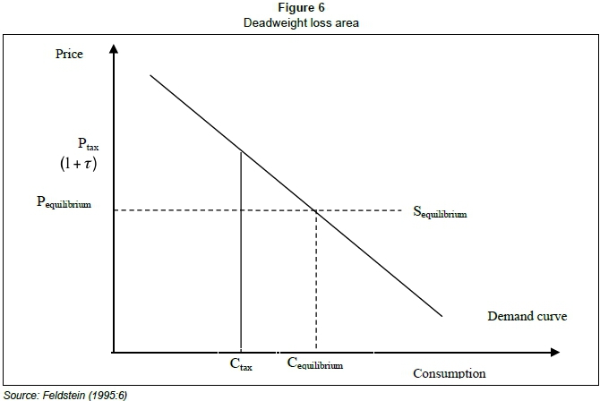
Figure 6 illustrates the derivation of the deadweight loss using the consumer-surplus methodology (Feldstein, 1995:4). The deadweight loss of PIT therefore depends on taxable income and the elasticity of taxable income. The deadweight loss changes with behavioural changes. So, if the tax rates increase to raise revenue, they affect the level of the deadweight loss as well.
4 Validation of the MS model results
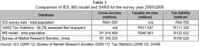
After simulating tax liability with the MS model, the results are compared with published SARS data, the IES, and data of the Bureau of Market Research of the University of South Africa. Table 3 shows that the MS model's tax liability of R132 billion exceeds the SARS assessed tax liability of R111 billion (the actual amount collected was R125 billion). This is plausible, since the MS model accounts for the whole of the South African population and not only for assessed taxpayers. The results for gross income and tax liability are very similar to those of the Bureau of Market Research (2000:17). It should be noted, though, that the MS model only calculates tax liability, which differs from the actual amount collected due to advanced and lagged payments.
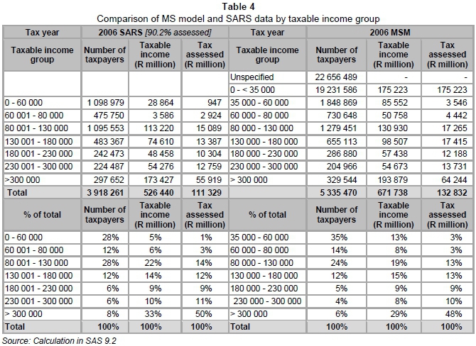
Table 4 shows the MS model results. Almost half of the population shows unspecified gross income, while approximately 19 million fall under the tax threshold of R35 000. About 1.8-million individuals earn income between R35 000 and R60 000. Those earning less than R60 000 only qualified for the Standard Income on Employees Tax (SITE) and were not liable to file a tax return. The base model results can be validated by comparing the aggregate output with the published SARS data in the Tax Statistics in Table 4. One would not expect identical results, but the aim is to show that the MS baseline results are broadly in line with the published data.
4.1 Tax reform - two scenarios simulating a more and less progressive marginal tax rate regime
As mentioned previously, the main objective with this analysis is to determine the impact of changes in marginal tax rates of individuals on the revenue base and on tax efficiency. The marginal tax rates for the 2005/2006 fiscal year are used as a base from which changes are implemented. Besides the base scenario, two other scenarios are simulated: one where marginal rates are increased and one where marginal rates are decreased. The three marginal tax rate structures are reported in Table 5. The scenarios are as follows:

Scenario A: This is the base scenario with marginal rates as in the 2005/2006 fiscal year. The marginal rate at the lower end is 18 per cent and 40 per cent at the highest end. It should also be mentioned that these rates have remained unchanged since the 2002/2003 fiscal year.
Scenario B: From the literature, it is evident that high-income countries' marginal tax rates are higher than those of upper middle-income countries. In order to choose a realistic scenario with higher marginal rates, the rates in South Africa that applied in the financial year 1998/1999 were used in the model. The scenario is useful, since, in that year, the number of income tax bands was reduced to six from the previous 10, making the comparison much easier. Marginal rates in this scenario range between 19 and 45 per cent for the lowest and highest income groups, respectively.
Scenario C: This scenario includes lower marginal tax rates. According to the literature discussed, the marginal tax rate for the lower-income band should be between 10 and 20 per cent, and the highest marginal tax rate between 30 and 50 per cent, with the number of income tax bands between four and six. Therefore, the scenario reflects a tax regime comparable with the tax regimes of South Africa's peers, with marginal tax rates starting at 12 per cent and increasing to a maximum of 30 per cent for the highest income group.
4.2 Impact on the revenue base and tax efficiency
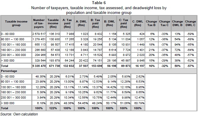
The results for the base Scenario (A) are given in Table 6, which reflects the number of taxpayers, taxable income, tax assessed, and the deadweight loss per population group for the different income groups. The total deadweight loss amounts to R37.5 billion, with total tax liability at R132.8 billion. Note that tax efficiency decreases (deadweight loss increases) with an increase in taxable-income levels. This decrease in efficiency is especially noticeable in the case of the highest income group (54.5 per cent increase in deadweight loss).
Table 6 also shows the results of both more and less progressive marginal tax rate regimes, compared with the base model. In Scenario B, the marginal tax rate per income group increases from 18 to 19 per cent, 25 to 30 per cent, 35 to 43 per cent, 38 to 44 per cent, and 40 to 45 per cent, respectively. These increases result in an increase in total revenue, from the previous R132.8 billion to R153.7 billion (an increase of 16 per cent), but with deadweight loss increasing from R37.5 billion to R56.2 billion (an increase of 50 per cent).
The decreased marginal tax rates in Scenario C (from 18 to 12 per cent, 25 to 15 per cent, 30 to 19 per cent, 35 to 23 per cent, 38 to 27 per cent, and 40 to 30 per cent, respectively) imply a loss of about R43 billion (tax liability decreases from R132.8 to R89.9 billion), but also a reduction in the deadweight loss by R21.3 billion. The changes in both revenue and deadweight loss per income group show that income groups are affected differently by changes in marginal taxes. Although those in the highest income group are most affected in absolute terms in both Scenarios B and C as far as tax liability is concerned, the percentage change is different from that of some of the other groups. In the case of Scenario B, the tax liability of those in the income group above R300 000 increases by 15 per cent, while their tax efficiency decreases by 38 per cent. In Scenario C, this group's tax liability decreases by 29 per cent and tax efficiency increases by 52 per cent. However, a similar analysis of the income group R130 000 to R180 000 demonstrates that, in the case of Scenario B, their tax liability increases by 18 per cent, but tax efficiency as measured by the inverse of the deadweight loss of tax in this income group decreases by 94 per cent. In Scenario C, with the lower rates, their tax liability decreases by 37 per cent and their deadweight loss by 65 per cent (increase in tax efficiency).
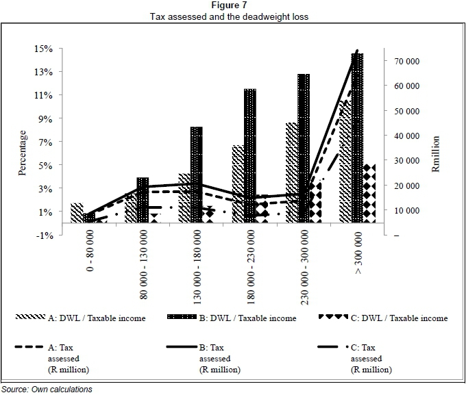
Figure 7 shows that both tax liability and the deadweight loss as a percentage of taxable income increase over all the taxable income groups. With higher marginal tax rates (Scenario B), tax revenue increases, but tax efficiency decreases. Lower marginal tax rates (Scenario C) show a decrease in tax revenue in all income groups, but an increase in efficiency.
Figure 8 shows that, in the base scenario, the deadweight loss as a percentage of total PIT amounts to 28 per cent, but, with a more progressive regime, it increases to 37 per cent, and, with a less progressive regime, it declines to 16 per cent. Note that Thomas (2007:23), in using the elasticity of taxable income with respect to tax rates (0.52), estimates the deadweight loss as a percentage of tax revenue at 15 per cent for New Zealand's flatter-rate system. For the United States, Robson (2007:15) summarises different studies and the ratio range between 18 per cent and 37 per cent.
As indicated earlier, the optimal growth-maximising tax ratio (PIT/GDP) where economic growth is maximised is estimated at 6.7 per cent. Figure 9 shows that, for Scenarios A and B, the PIT/GDP ratios are 8.2 and 9.6, respectively, which are higher than the optimal ratio. With less progressive marginal tax rates, the PIT/GDP ratio declines to 5.6, which is less than the optimal tax ratio, and it can be assumed that such a policy reform would stimulate economic growth and thereby expand the revenue base to compensate for the first-round loss in revenue.

5 Conclusion
Of all the tax-policy scenarios tested in this study, the one that appears to have the most potential to positively impact on economic growth realigns marginal tax rates to levels closer to those of South Africa's peers. Such a policy intervention is also very relevant given the trend in tax globalisation and the resultant international tax competition for a developing country such as South Africa. Studies show that several countries have embarked on a declining trend in marginal tax rates on personal income. As a general guideline, it is proposed that the top maximum marginal rates should vary between 30 and 50 per cent, with minimum rates between 10 and 20 per cent. Currently, the rates for upper middle-income countries average about 9 per cent for the lowest income category to about 29 per cent for the highest category (SADC countries: 30 per cent). In South Africa, the current minimum and maximum marginal rates are 18 and 40 per cent, respectively, which are clearly higher than those of its peers.
When the model is adjusted, it reflects that the most favourable scenario for reaching the optimal PIT/GDP ratio of 6.7 per cent is to lower marginal rates. In fact, when the marginal rates are lowered to the averages of South Africa's peers (12 to 30 per cent), the PIT/GDP ratio will actually decrease to only 5.6 per cent. Obviously, the corresponding loss in revenue will have to be compensated for, but basic theory explains that, in the longer term, the revenue base will be broadened as a result of the efficiency gains that exceed the loss in revenue. Although not tested in the model due to its stationary nature, it is expected that such a loss in revenue would be covered by an increase in productivity and capital flows that further advance economic growth and thereby expand the revenue base. It has also been concluded that such a realignment of marginal rates will benefit taxpayers primarily in the middle-income groups, which comprise a large cohort of South African employees. For example, the analysis for the income group R130 000 to R180 000 demonstrates that, with the lower rates suggested, tax liability decreases by 37 per cent while tax efficiency increases by 65 per cent. Should the tax authorities in South Africa target the optimal PIT/GDP growth level (6.7 per cent), the decline in marginal rates do not have to be as extreme as indicated and will reduce the revenue loss, but, obviously, also reduce the gain in efficiency.
The authors acknowledge the fact that tax-policy recommendations as outlined in this study have to be dealt with carefully given the complexity of the impact of such policy changes. It is therefore advised that, in follow-up studies, the quality of the results be further substantiated by linking this model to a dynamic CGE model, which would improve on the quantification of the secondary impact of tax adjustments on the economy's performance, such as job creation and revenue. Furthermore, it is also acknowledged that historic events such as the policy of "apartheid" have impacted negatively on the structure and composition of the revenue base of South Africa, with the result that comparisons with peer countries are rather complicated. Accordingly, policymakers have to discount these caveats when considering the policies recommended in this study and carefully weigh the trade-offs between lower levels of personal tax income and the benefits of increased tax efficiency and economic growth.
References
ATKINSON, A.B., PIKETTY, T. & SAEZ, E. 2011. Top incomes in the long run of history. Journal of Economic Literature, 49(1):3-71. [ Links ]
BALLARD, C.L., FULLERTON, D., SHOVEN, J.B. & WHALLEY, J. 1985. Introduction to "A general equilibrium model for tax policy evaluation". A general equilibrium model for tax policy evaluation. University of Chicago Press. [ Links ]
BARLETT, B. 2012. What is the revenue-maximizing tax rate? Tax Notes, 134:8. Available at: http://ssrn.com/abstract=2008750 or http://dx.doi.org/10.2139/ssrn.2008750 [accessed 2012-07-23]. [ Links ]
BIRD, R.M. 2008. Tax challenges facing developing countries. International Center for Public Policy (formerly the International Studies Program) Working Paper Series, at AYSPS, GSU paper 0802. [ Links ]
BUDDELMEYER, H., CREEDY, J. & KALB, G. 2007. Tax policy - design and behavioural microsimulation modelling. Cheltenham, UK & Northampton, MA, USA: Edward Elgar Publishing Limited. [ Links ]
BUREAU OF MARKET RESEARCH BUNDLES. 2000. Personal disposable income in South Africa by population group, income group and district. Pretoria: University of South Africa, Bureau of Market Research. Research report no. 279. [ Links ]
CITRO, C.F. & HANUSHEK A. 1991. Improving information for social policy decisions: The uses of microsimulation modeling. Washington, D.C.: National Academy Press. [ Links ]
CREEDY, J. 2010. The elasticity of taxable income: An introduction. Public Finance and Management, 10:556-589. [ Links ]
FAN, X., FELSÖVÄLYI, A. & KEENAN, S. 2002. SAS for Monte Carlo studies: A guide for quantitative research. SAS Institute. [ Links ]
FELDSTEIN, M. 1995. The effect of marginal tax rates on taxable income: A panel study of the 1986 Tax Reform Act. Journal of Political Economy, 103:551-572. [ Links ]
FELDSTEIN, M. 2011. The tax reform evidence from 1986. Wall Street Journal. Available at: http://www.nber.org/feldstein/wsj10242011.html [accessed 2012-07-14]. [ Links ]
GWARTNEY, J.D. 2008. Supply-side economics. The concise encyclopedia of economics. David R. Henderson (ed.) Liberty Fund, Inc. Library of Economics and Liberty. Available at: http://www.econlib.org/library/Enc/SupplySideEconomics.html [accessed 2012-07-14]. [ Links ]
HASSAN, F.M.A. & BOGETIC, Z. 1996. Effects of personal income tax on income distribution: Example from Bulgaria. Western Economic Association international contemporary economic policy. Volume XIV. [ Links ]
IMMERVOLL, H. & O'DONOGHUE, C. 2009. Towards a multi-purpose framework for tax-benefit microsimulation: A discussion by reference to EUROMOD, a European tax-benefit model. International Journal of Microsimulation, 2(2):43-54. [ Links ]
LEHMER, D.H. 1951. Second Symposium on large-scale digital calculating machinery. Cambridge: Harvard University Press:141-146. [ Links ]
NATIONAL TREASURY. 2003. Budget review. Pretoria: Department of Finance. [ Links ]
NATIONAL TREASURY. 2006. Budget review. Pretoria: Department of Finance. [ Links ]
NTSONGWANA, P., WRIGHT, G. & NOBLE, M. 2010. Supporting lone mothers in South Africa: Towards comprehensive social security. Available at: http://www.casasp.ox.ac.uk/docs/Lone%20Mothers%20and%20Comprehensive%20Social%20Security.pdf [accessed 2012-05-18]. [ Links ]
OECD. 2012. Economic policy reforms 2012: Going for growth. OECD Publishing. Available at: http://dx.doi.org/10.1787/growth-2012-en [accessed 2012-06-03]. [ Links ]
PEICHL, A. & SCHAEFER, T. 2009. FiFoSiM - an integrated tax benefit microsimulation and CGE model for Germany. International Journal of Microsimulation, 2(1):1-15. Available at: http://www.microsimulation.org/IJM/V2_1/IJM_2_1_1.pdf [accessed 2010-03-19]. [ Links ]
PETER, K.S., BUTTRICK, P. & DUNCAN, D. 2009. Global reform of personal income taxation 1981-2005: Evidence from 189 countries. Available at: http://www.econstor.eu/dspace/bitstream/10419/35825/1/605989540.pdf [accessed: 2012-10-01]. [ Links ]
ROBSON, A. 2007. No free lunch the cost of taxation. New Zealand Business Roundtable, Wellington, New Zealand. [ Links ]
SARB (South African Reserve Bank). 2012. Quarterly Bulletin (various issues). Pretoria. [ Links ]
SAUNDERS, P. 2007. Taxploitation: The case for income tax reform. Published by the Centre for Independent Studies. [ Links ]
SAUTORY, O. 1993. La macro CALMAR: Redressement d'um echantillion par calage sur marges. Working Paper no. F9310. Institut National de la Statistique et des Etudes Exconomiques. [ Links ]
SCHOEMAN, N.J. & VAN HEERDEN, Y. 2009. Finding the optimum level of taxes in South Africa: A balanced budget approach. South African Journal of Industrial Engineering, 20(2): 15-31. [ Links ]
SCULLY, G.W. 1991. Tax rates, tax revenues and economic growth. Policy Report 98. Dallas, TX: National Center for Policy Analysis. [ Links ]
SCULLY, G.W. 1994. What is the optimal size of government in the United States? Policy Report 188. [ Links ]
STATISTICS SOUTH AFRICA. 2005. Mid-year population estimates 2005 to 2006: Statistical release P0302. Available at: http://www.statssa.gov.za/publications/statspastfuture.asp?PPN=P0302&SCH=4696 [accessed 2012-07-14]. [ Links ]
STATISTICS SOUTH AFRICA. 2008. Income and expenditure of households 2005/2006: Statistical release P01001. Available at: http://www.statssa.gov.za/publications/statsdownload.asp?PPN=P0100&SCH=4108 [accessed 2012-01-03]. [ Links ]
STEENEKAMP, T.J. 2012. The progressivity of personal income tax in South Africa since 1994 and direction for tax reform. Southern African Business Review, 16(1):39-57. [ Links ]
ŠTĔPÁNKOVÁ, P. 2002. Using microsimulation models for assessing the redistribution function of a tax- benefit system. Finance a úivěr', 52(1):36-50. [ Links ]
TAX STATISTICS. 2009. National Treasury and the South African Revenue Service. Pretoria. [ Links ]
TAX STATISTICS. 2010. National Treasury and the South African Revenue Service. Pretoria. [ Links ]
THOMAS, A. 2007. Taxable income elasticities and the deadweight cost of taxation in New Zealand. Unpublished paper, Inland Revenue, Wellington. [ Links ]
USAID. 2011. USAID leadership in public financial management project: Collecting taxes Full data. [ Links ]
Accepted: April 2015
1 Primary income (2005/2006) = [(1 070*10/12) + (1 190 *2/12)]*93%.
2 Primary income (2005/2006)/IES gross income = 1 014 billion/749 billion.
3 A more comprehensive description of the methodology is contained in the author's thesis which is to be available soon.

