ARTICLES

 

A primer on counterparty valuation adjustments in South Africa

 

 

Gary van Vuuren; Ja'nel Esterhuysen

School of Economics, North West University

 

 

---

ABSTRACT

Counterparty valuation adjustment (CVA) risk accounts for losses due to the deterioration in credit quality of derivative counterparties with large credit spreads. Of the losses attributed to counterparty credit risk incurred during the financial crisis of 2008-9 were due to CVA risk; the remaining third were due to actual defaults. Regulatory authorities have acknowledged and included this risk in the new Basel III rules. The capital implications of CVA risk in the South African milieu are explored, as well as the sensitivity of CVA risk components to market variables. Proposed methodologies for calculating changes in CVA are found to be unstable and unreliable at high average spread levels.

Key words: counterparty credit risk, CVA, credit ratings, Basel III

---

 

 

1 Introduction

The 2008-2009 financial crisis originated when asset price bubbles inflated, interacting with new kinds of financial innovations that masked risk (Baily, Litan & Johnson, 2008). In December 2010, the Basel Committee on banking supervision (BCBS) updated Basel II with a set of rules known as Basel III (BCBS, 2011) designed to augment and repair the Basel II rules which did not function effectively in the financial crisis. Amongst these are new regulations for CVA and CVA risk.

The traditional approach to control counterparty credit risk was to establish limits against future exposures and verify potential trades against these limits - these are commonly referred to as potential future exposures (PFEs) (Algorithmics, 2012). The severe volatility experienced during the financial crisis, however, led to a comprehensive review of accounting for counterparty credit risk (CCR). As a result, the value of derivatives transactions with counterparties is now adjusted by dealers to reflect the possibility of loss incurred because of counterparty default (Hull & White, 2012). This adjustment is known as the credit value adjustment (CVA). CVA eliminates the need for controlling CCR through limits by introducing dynamic CCR pricing directly into new trades. Many banks already take CVA into account in their accounting statements, but the financial crisis has led innovative banks to more accurately assess CVA, and integrate CVA into pre-deal pricing and structuring. Calculating CVAs is, however, computationally intensive (Pykhtin & Zhu, 2007: Gregory, 2009a).

In addition to the measurement of CVA, CVA risk arises from changes in (a) counterparty credit spreads and (b) market variables that affect the no-default value of derivative transactions (Hull & White, 2012). CVA risk, therefore, may only be accurately assessed after the effect of changes in both components have been identified and measured. While Basel III requires an assessment of CVA risk arising from changes in counterparty credit spreads to be included in the market risk capital calculation, CVA risk - arising from changes in underlying market variables - is not required under Basel III.¹ This article explores the impact of CVA risk on regulatory capital requirements for banks and examines the influence of high spread levels on the accurate assessment of CVA risk.

This paper proceeds as follows: Section 2 provides a broad literature review explaining the concept of CCR, its importance in modem finance, why CVA is necessary and problems with the concept of CVA and its practical implementation. Section 3 covers the various methodologies proposed by several authors to measure CVA and provides a synthesis of these methodologies into a coherent approach for the South African market. In addition, this section details the data requirements and establishes the requisite mathematics for measuring CVA. Due to the calculation complexity involved in determining portfolio CVA, a single, simple interest rate derivative was used as the underlying derivative transaction to explain the processes involved. The results obtained from models proposed in Section 3 are provided in Section 4, along with a discussion of these results and an interpretation of model strengths and weaknesses. The influence of changes in average spread levels on CVA is explored and found to be counterintuitive and potentially inaccurate if applied indiscriminately. The effect of changing underlying market factors on risk capital is also investigated, despite the omission of this effect from Basel III rules. Using South African data, specific attention is paid to the South African market. Section 5 proposes future research and concludes.

 

2 Literature review

It became apparent in the 1990s that over the counter (OTC) derivatives trading gave rise to significant credit risk exposure (Canabarro & Duffie, 2003). Banks implemented two principal measures to deal with this risk: risk reduction via enforced close-out netting agreements with (or collateral posting from) the relevant counterparty and risk pricing by charging counterparties a spread, dependent on the riskiness (for example, credit rating, maturity) of the transaction. This charge - the CVA - is minimal for a transaction in which the collateral is exchanged daily, in cash, on the full mark-to-market of the derivative portfolio, but it can be substantial if the counterparty is not obliged to post collateral, and particularly if the credit quality of the counterparty is poor (for example, rated subinvestment grade or worse than BB-).

Currently (2014), the majority of a typical bank's CVA comprises two classes of counterparty namely sovereigns (which traditionally do not post collateral despite their substantial derivatives trades) and corporates (which unlike most banks, are often not in a position to move collateral every day). These corporates may be willing to post collateral less frequently, but resent such restrictions on cash flows and often demand that banks only request collateral when requirements exceed a certain threshold (Hull & White, 2012). Individual CVAs may be insubstantial, but the total CVA for banks' corporate derivatives books can be extensive.

Canabarro & Duffie (2003) introduced methodologies to measure, mitigate and price CCR. Monte Carlo simulation techniques were proposed as a pricing mechanism for CCR and a practical estimation of CVA using currency and interest rate swap trades between two defaultable counterparties was presented.

Portfolio level counterparty risk and credit mitigation techniques were discussed by De Prisco & Rosen (2005) who also employed Monte Carlo simulation to calculate statistics relevant to CCR measurement. A practical implementation of collateral modelling was proposed. The measurement of the expected exposure in credit derivative portfolios was also affected by wrong way risk. (Wrong way risk arises when the exposure to a counterparty is positively correlated with the credit quality of that counterparty, so default risk and credit exposure increase together).

Gibson (2005) discussed both an analytical and a Monte Carlo simulation method to measure expected exposure and expected positive exposure for margined and collateralised counterparties. The former method uses a Gaussian model to determine the mark-to-market value of a portfolio exposed to counterparty risk. The latter simulation method however uses a Gaussian random walk to explore the relationship between collateralised exposures and other variables, such as the initial mark-to-market, the threshold, and the re-margining period.

Redon (2006) presented two analytical methods to measure expected exposure subject to wrong way risk. The first calculates expected exposure as a weighted average of expected exposure in the presence and absence of country crises, while the second - based on a Merton model² of default risk - estimates expected exposure by assuming Brownian motion to model the mark-to-market value of the portfolio subject to counterparty risk. Correlating the Brownian motions used to model both default and mark-to-market allow the determination of wrong way risk and the derivation of analytical expressions for expected exposure.

Pykhtin & Zhu (2007) demonstrated how margin agreements may be employed to reduce CCR and, through the exploration of differences between counterparty and contract-level exposures, presented a methodology for calculating expected exposure and CVA assuming wrong way risk.

Bilateral counterparty risk was discussed in detail by Brigo & Capponi (2008) who demonstrated that in the absence of spread volatility, CVA decreases as the correlation between investor and counterparty tends to 1. Modelling the joint default of the investor, counterparty and underlying credit default swap (CDS) led to the conclusion that pure contagion models may not be appropriate for modelling CVA risk in high correlation environments. The authors also concluded that simple add-on approaches to capture CVA behaviour (such as those described by the BCBS, 2006) were ineffectual.

Gregory (2009b) calculated bilateral CVA for a portfolio comprising OTC derivatives. A Gaussian copula model which permitted simultaneous defaults was used and the effect of these defaults (which effectively represent systematic risk) on the measured CVA, was shown to be insignificant.

Using a structural model subject to jump diffusion, Lipton & Sepp (2009) explored CCR in CDS contracts. From their results, novel techniques were developed for measuring CVA.

A Markov portfolio credit risk model which accounts for default and wrong way risk dependence by allowing simultaneous defaults among underlying credit names, was proposed by Assefa, Bielecki, Crépey & Jeanblanc (2009). Employing the standard assumption of no dependence between exposure and probability of default, a relationship between the counterparty's hazard rate and the value of variables was specified, whose values can be generated by Monte Carlo simulation (and used to calculate CVA). The results obtained show good agreement between the behaviour of expected positive exposure and CVA (Assefa et al., 2009).

Other authors who tackled the wrong-way risk problem include Cespedes, De Juan Herrero, Rosen & Saunders (2010) and Sokol (2010) who both approached the problem by assuming the exposure follows a one-factor Markov process and a copula (Gaussian or otherwise) determines the dependence between this process and the time to default.

CVA losses were considerable for some banks during the credit crisis. Under Basel II, the risk of counterparty default and credit migration risk were addressed, but mark-to-market losses due to CVA were not (i.e. CVA risk had no capital assigned to it). Roughly two-thirds of losses attributed to CCR during the financial crisis, however, were due to CVA losses. Only about one third were due to actual defaults (BCBS, 2011). Basel III now includes charges for CVA risk designed to ensure that banks carry substantial amounts of capital against CVA risk - particularly for over-the-counter derivatives trading with counterparties who do not post daily cash collateral. It is important to note that the new capital does not provide for the risk of loss due to counterparty default, but rather the risk that the CVA might increase (Hull & Wihte, 2012).

A separate but related problem involves central counterparties (CCPs). In 2009, the Group of 20 mandated local regulators to route a portion of derivative trades through domestic central counterparties (CCPs) (Group of 20, 2009). In part because this exercise involves co-operative cross-border regulatory schemes, most large international markets (including the Eurozone, Australia, Hong Kong and Canada) have retreated from the directives, stating "concerns of domestic supervisors" (Wood, 2013).

South African derivative dealers are active and enthusiastic participants of international markets and must, therefore, address clearing mandates of international dealers despite the absence of a domestic CCP (February 2014).³ South Africa is also committed to the successful implementation of Basel III which includes CVA capital charges (and thus clearing incentives for derivative counterparty risk). Understanding the vagaries of CVA is thus of critical importance to the South African derivatives market (Wood, 2013).

 

3 Methodology and data

Since all derivatives involve counterparties, valuation of derivative transactions must take into account the possibility of loss incurred because of counterparty default (Hull & White, 2012).

CVA is thus a cost. To measure CVA and ultimately the CVA risk associated with derivative transactions, the underlying deriva-tive(s) must first be valued. In practice, banks will more likely trade portfolios comprising several derivatives, but for this article, a single, simple interest rate swap was used. This serves the triple purpose of (a) providing a basis for the complete CVA calculation without the introduction of unnecessary complexity, (b) calibrating the South African yield curve using the Vasicek mean reverting interest-rate model and (c) elucidating the effects of elevated credit spread levels on CVA.

3.1 Construction and calibration of the South African yield curve

Yield curve models are divided into two principal types: equilibrium approaches and no-arbitrage models. The former focus on modelling the dynamics of the instantaneous rate. Yields at longer maturities are then derived using assumptions about the risk premium. Equilibrium models focus primarily on time-series dynamics at the expense of inaccurate fitting of the complete cross-section of the yield curve. The latter models emphasise perfect fitting of the term structure at points in time so as to guarantee that no arbitrage possibilities exist. Although these models are of particular importance for pricing derivatives, they ignore time series dynamics of the yield curve which can be important for bond pricing and other fixed-income securities (Diebold & Li, 2006).

The Vasicek model - which follows the equilibrium tradition and an early proponent of term structure models - appeared in 1977. Subsequently, it has survived and inspired several other models and it remains of considerable importance in valuing securities that require accurate time-series dynamics, including bond options, futures and other interest rate derivatives (Vasicek, 1977; Mamon, 2004). A key innovation of the Vasicek model, supported and justified through economic arguments, was the introduction of a mean-reverting stochastic process to model the evolution in time of the short rate. The model assumes that the current short rate is known with certainty and its subsequent evolution is governed by (Vasicek, 1977):

where the current short rate, r_t is a continuous (no jumps) function of time and follows a Markovian diffusion process, γ is the long run mean of the short rate, a is a measure of the speed of the return of the short rate to the long run mean (the mean reversion coefficient), σ is the short rate volatility and zt is a standard Wiener process. Research has relaxed the condition of constant volatility (Brenner, Harjes & Knoner, 1996; Hong, Li & Zhao, 2004) and Shimizu and Yoshida (2006) have adapted Equation 1 to include diffusion processes with jumps.

The parameters of Equation (1) (α,γ and σ) were estimated using maximum likelihood methods (James & Webber, 2004) and historical South African data spanning 2001 - 2013 procured from South African banks. Discount factors (used to price the interest rate swap -see Section 3.2) were calculated from (Hull & White, 1990, 1995):

where

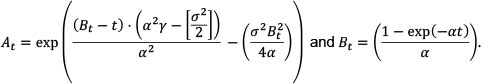
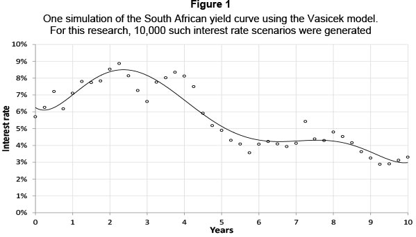
Figure 1 shows the term structure (up to 10 years) of one possible yield curve constructed using the Vasicek model. Relevant parameters were derived directly from the South African market.

3.2 Pricing a simple interest rate swap

A simple floating rate note (FRN) was used to price the interest rate swap. The FRN pays a floating rate coupon / at the end of each coupon period h and the accrual period is the same for all coupons. The floating rate is fixed at the prevailing market rate, for the i^th coupon period, at the beginning of each coupon period t_i. The floating rate thus corresponds to the forward rate between t_i and t_i + h measured at time t_i. The present value of the FRN today is the expected value of the future floating cashflows plus the principal at maturity. Future forward rates,/(t_i, t_i, t_i + h), are unknown, but these may be set equal to today's expected forward rates /(0, t_i, t_i + h) using the principal of no arbitrage.⁴ The FRN value is the present value of the sum of N expected floating rate coupons, f_ih, plus principal:

with the i^th forward rate given by / = /(0, t_i, t_i + h) and DF the relevant discount factors (Vasicek, 1977).

The value of this FRN (assumed to have no credit risk exposure) can be shown to equal par (i.e. 100 per cent) by substituting the definition of the forward rate (Equation 4, below) into Equation 3:

Simple fixed/floating interest rate swaps may be represented by a series of fixed (or floating rate) payments, exchanged with a counterparty into a series of floating (or fixed) rate cash flows. Such a swap - paying a fixed rate C plus principal and receiving a floating rate plus principal - is used as the underlying derivative in this paper (Vasicek, 1977).

Assume j = 1, ..., N floating coupons with accrual periods hj and i = 1, ..., M fixed rate coupons with coupon period l_i. The principal amounts are the same on both sides of the swap, so they cancel and:

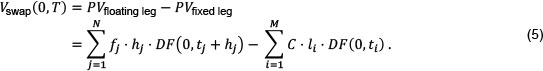
Market rate swaps are constructed such that the initial mark-to-market value is zero, thus the fair market coupon (annualised swap rate R(0,T) for maturity T) may be derived by rearranging Equation (6) to solve for the swap rate R(0,T) = C:

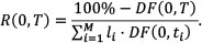
The market swap rate, R(0,T), is the swap level conventionally quoted in the market (Vasicek,1977). This rate is the annualised fixed rate paid or received on a market swap with a given maturity T. Note that the discount factors, DF, are calculated using Equation 2.

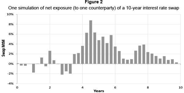
Figure 2 shows the net exposure (to one counterparty) of a 10-year interest rate swap as a percentage of notional associated with the simulated yield curve in Figure 1. For this research, 10,000 such exposure profiles were generated corresponding to the 10,000 interest rate scenarios.

3.3 CVA calculation

CVA is the market value of counterparty credit risk: the difference between the risk-free portfolio value and the true portfolio value that takes into account the counterparty's default. When there are netting and collateral agreements, CVA must be calculated at the counterparty level and not separately for each individual trade (Hull & White, 2012).

In addition to modelling limitations, calculating CVA is computationally intensive. It is now standard for banks to employ Monte Carlo simulations to compute counterparty exposures. This is the most expensive step: A single simulation of a portfolio of 50,000 positions, over 2,000 scenarios and 100 time steps, requires 10 billion valuations. A comprehensive risk analysis requires a large number of CVA calculations for sensitivities, CVA VaR and marginal CVA of new trades (Rosen & Saunders, 2012).

CVA can be defined either on a unilateral or a bilateral basis. Unilateral CVA assumes that the institution which does the CVA analysis (the bank) is default-free. It gives the market value of future losses caused by the counterparty's potential default. Bilateral CVA takes into account the possibility of both the counterparty and the bank defaulting. This is required for an objective fair value calculation since both bank and counterparty require a premium for the credit risk they bear, otherwise, they would not agree on the fair value of the trades. Unilateral CVA is now part of Basel III, (BCBS, 2009) while bilateral CVA is more in line with the market practice at top financial institutions for pricing and hedging, as well as accounting rules (FASB, 2006).

Assuming no wrong way risk (equivalent to assuming that the default probability, exposure and recovery values are independent), CVA is given by:

where R is the recovery rate, ((1 - R) is the loss given default), B(tj) is the risk-free discount factor at time tj, EE(tj) is the expected exposure at time tj, q(tj_-1, tj) is the marginal default probability in the interval [tj_-1, tj] and where m is the maturity (Gregory, 2009b). Note that default is present in Equation 6 only via default probabilities, thus when employing a simulation framework to estimate CVA, only exposures need to be simulated, not default events (which are rare) (Gregory, 2009b).

3.4 Estimating the components of the CVA calculation

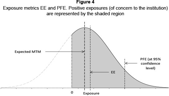
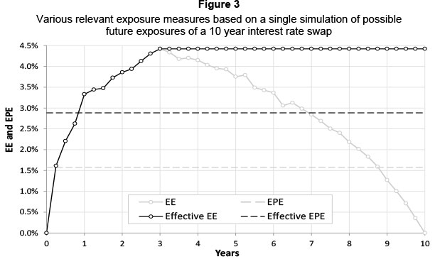
Expected exposures are the probability-weighted positive exposures: calculating these is a non-trivial exercise. Consider the positive exposure profile for a 10 year interest rate swap in Figure 3 below. The effective exposure (EE) is the positive mark-to-market value (since it is only these exposures - the positive mark to market (MtM) values - which are of concern to the institution since losses will only occur for these exposures) of an institution's exposure to a counterparty. The expected positive exposure (EPE) is the average EE through time while the effective EE is the non-decreasing EE: the value ratchets up, never down, over the derivative's lifetime. The effective EPE is the average of the effective EE. Note that future exposures are simulated, thus the potential future exposure (PFE, not shown in Figure 3) is the exposure exceeded with a given probability (usually 95 per cent or 99 per cent). If 1,000 simulations of possible future exposure profiles are generated, the PFE is the 50^th largest exposure at a 95 per cent confidence level. In principle, this is similar to the well-known and widely used historical value at risk methodology in market risk.

The EE represents the expected (probability-weighted) exposure value conditional to being in the shaded area (i.e. exposure > 0) in Figure 4 below.

 

 

To estimate the value of EE analytically, consider a normal distribution with mean μ and standard deviation σ where the former represents the expected mark-to-market value of the derivative value (or the portfolio of derivatives) and the latter represents the standard deviation of these mark-to-market values. The mark-to-market value, V, of this transaction at any time t is given by V = μ + σΖwhere Z is a standard normal variable. It follows that the (positive) exposure, E, may be written as E - max (V,0) = max (μ + σΖ, 0). The expected exposure in this case is:

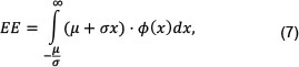
and where the lower integration limit is from μ + σΖ, hence

Integrating Equation 7 gives:

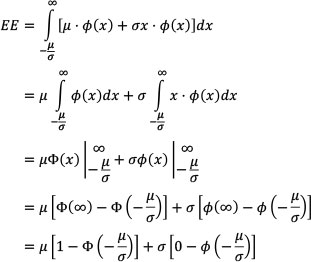
Hence

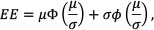
where φ(...) is the normal distribution function, φ(...) is the cumulative normal distribution function and use has been made of the fact that 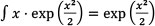and To generate the results required, 10,000 interest rate scenarios (and associated exposure profiles for each scenario) were generated using Monte Carlo simulation.

Recovery rates are assumed to be constant. Although this condition may be relaxed, recovery rates are notoriously difficult to estimate practically, so this assumption is not unusual (e.g. Gregory, 2009b, Hull & White, 2012).

Risk neutral discount factors are determined using Equation 2, which are - in turn -based on an interest rate model (in this case, a mean-reverting, Vasicek interest rate model).

Marginal probabilities of default may be calculated from credit spreads. If the complete term structure of credit spreads for the relevant counterparty cannot be observed in the market this may be estimated using credit spread data for similar companies (in the same sector, for example, and preferably operating in the same geography). A reasonable estimate of the risk neutral marginal probability, q(0,j), between times 0 and tj is given by where Sj is the credit spread for a maturity of tj. It follows that the marginal risk neutral probability of default - defined by qj - may be given by:

Swap values were obtained from one of the 'Big 4' South African retail and commercial banks.

With the components of Equation 6 established, these are combined and the results obtained presented in the following section.

 

4 Results

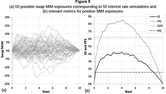
Of the 10,000 possible exposure profiles generated from the 10,000 interest rate scenarios, (for clarity) only 50 are shown in Figure 5(a) below. Figure 5(b) illustrates the expected exposure, the potential future exposure and the expected (average) values of each of these swap MtM metrics.

 

 

4.1 Effect of credit spread changes on CVA

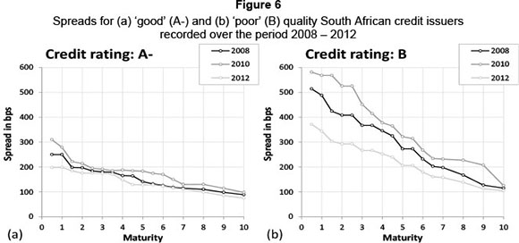
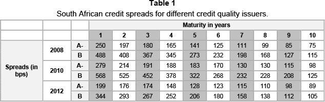
Credit spreads for maturities up to 10 years for South African issuers of differing credit quality are shown in Table 1, spanning from the onset of the crisis in 2008 until December 2012. Credit spreads were at their highest levels, during the European sovereign crisis in 2010, but have since recovered. These data provide an indication of levels to which credit spreads may rise. It is likely that worse credit quality issuers suffered even higher spreads.

The spreads for these different quality issuers -spanning 5 (2008-2012) turbulent years - are shown in Figure 6 below.

 

 

Using Equations 6 and 8, the CVA for a 10-year, OTC interest rate swap with payments netted off and settled on a quarterly basis, was calculated using South African spreads derived from the recent market (December 2012) and as shown in Table 1 (in basis points (bps)).

The results obtained compare favourably with those estimated from other studies conducted in similar markets (see, for example, Carlson & Silén, 2012). CVA for low spreads (2012) high spreads (2008-10) is shown in Figure 7.

 

 

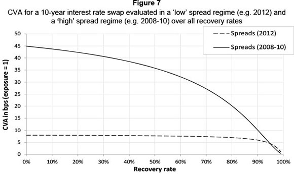
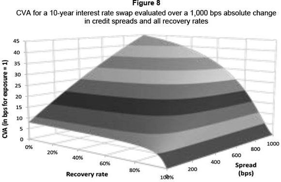
The CVA for different credit spreads, seen in Figure 7, was measured over all recovery rates (i.e. 0% < RR < 100%). Using a recovery rate of 55 per cent,⁵ the CVA is roughly three times higher when spreads are wide than when spreads are tight. At low recovery rates, the effect is more dramatic (up to six times greater). Figure 8 shows the full relationship of CVA to recovery rates and the absolute spread level.

 

 

4.2 CVA risk: changes in spreads

CVA is affected by two types of exposures: one from movements in counterparty credit spreads and the other from movements in underlying market variables. Considering the former, the impact on the CVA of a small change in spreads (As) over all s_i (i.e. a small parallel shift) may be estimated using a delta/gamma approximation, i.e. Δ/(χ) = ! · Δχ + ! Γ · (Δχ)² where δ = df / dx and Γ = d²f / dx² (Hull & White, 2012). Using Equation 6, the change in CVA is:

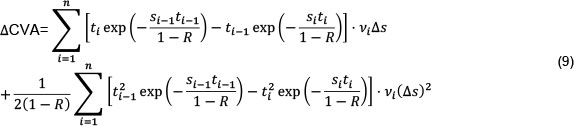
Note that Equation 9, the ACVA, is affected by changes in spreads (As) and the absolute spread level. The influence of both the change in spread and the absolute spread level is shown in Figure 9. To remain consistent with BCBS senior debt LGD values (BCBS, 2009), a fixed recovery rate of 55 per cent was chosen for this analysis.

 

 

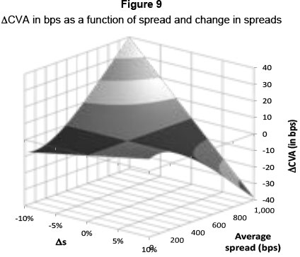
The results of Figure 9 pose some interesting questions. For low average spreads (such as those enjoyed by good quality credits during benign economic periods), as expected, CVA increases with increasing s. However, for high levels of average spreads (i.e. poor quality credits in volatile market conditions), an increase in spreads results in a decrease in CVA. It is difficult to believe these results were a deliberate attempt by this approach's proponents to restrict potentially punitive regulatory capital charges when markets are volatile and spreads are high.

Capital equations governing the Basel II Internal Ratings Based (IRB) approach for credit risk reduce the amount of regulatory capital required for unexpected credit losses at high probabilities of default (i.e. for PDs > 40 per cent, see Laurent, 2004) which seems counterintuitive at first glance. The resolution of the paradox, however, is fairly simple. At a given confidence interval⁶ total credit losses are the sum of expected and unexpected losses: the former are covered by bank pricing and provisioning and these increase with PD at a rate faster than regulatory capital (which covers unexpected losses) increase. As PDs increase, therefore, regulatory capital, covering unexpected losses, decrease since expected losses become more 'expected' and bank impairments increase faster. This logic cannot be applied to the shape of the ACVA versus As curves (higher spreads should result in higher CVA regardless of average spread). Ignorance of this could be detrimental to banks reserving capital for potential CVA losses, especially in highly volatile market conditions. Using this model (albeit when applied to the problem of wrong way risk), Hull & White (2012) found similar issues and argued that the sign of the calculated effects were counterintuitive.

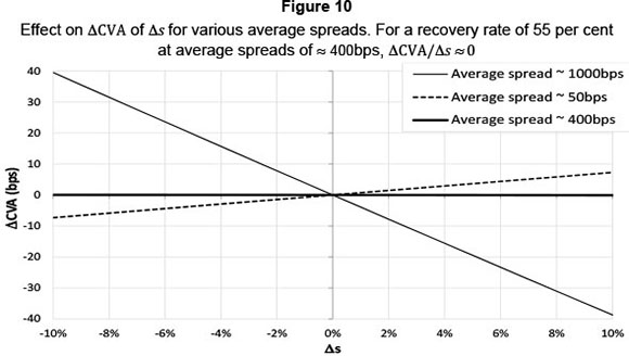
The slope of ACVA versus As changes sign (for a recovery rate of 55 per cent) when the underlying credit has an average spread of ≈ 400bps. As shown in Figure 10, at this average spread, the change in CVA for changes in spreads is negligible. These average spread levels are not rare (see Figure 6 and Table 1): they are commonplace for low maturity, poor quality credits or during stressed market conditions. That the proposed methodology suggests no increase in CVA for any changes in spread at these average spread levels, requires further investigation. The results at higher average spreads (namely that CVA decreases for increasing changes in spreads) is patently incorrect and potentially highly damaging.

 

 

4.3 CVA risk: changes in underlying market variables

Establishing the influence of small parallel variations in counterparty credit spreads on CVA and risk capital is a simple exercise using Equation 9. To accomplish the same for changes in underlying market variables is more complex since they evolve in time via geometric Brownian motion paths or mean reversion processes. The simulation dynamics for each is quite different.

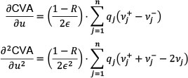
Using Equation 6 and rewriting B(tj) ^.EE(tj) as Vj, consider a market variable u with an initial value of u₀. Assume Vj changes to v_j⁺ and v_j^- when u₀ changes by a small amount, to u₀ + or u₀ - respectively. The associated partial derivatives of Equation 6 are:

Hull & White (2012) provide a discussion on the challenges posed by these complexities and offer an alternative way of measuring wrong way risk. Wrong way risk may be modelled by changing the way the VjS are calculated, but the calculation of the q(t)s (Equation 8) may be altered to incorporate the way variables used in the Monte Carlo simulation - discussed in Section 3 and used to determine CVA -evolve. To accomplish this, Hull & White (2012) introduce hazard rates: direct measures of the probability of default and although hazard rates are not observable in the market, they are related to credit spreads which are observable. A commonly-used approximation for the average, risk-neutral hazard rate between time 0 and t is:

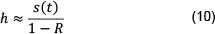
Where S(t) is the credit spread for maturity t.

Hull & White (2012) asserted that a counterparty's hazard rate may be modelled using a deterministic or stochastic variable that (a) affects the exposure to the counterparty and (b) can be calculated in the Monte Carlo simulation (Section 3). Potential candidate variables include credit spreads, share prices, relevant commodity prices (e.g. the oil price for an oil producer, the gold price for a gold producer, etc.). A robust relationship which satisfied the constraints outlined above was found to be:

Where a(t) is a function of time, the constant parameter b is a measure of the right-way (defined as the situation in which exposure to a counterparty is negatively correlated with the credit quality of that counterparty. So default risk and credit exposure move oppositely). A wrong way risk in the model is where w(t) is the value of the portfolio with the relevant counterparty, the constant σ measures the noise implicit in the model and e is a normally distributed such that e - N(0,1). Hull & White (2012) found that unless σ >> w(t), the noise term σe is negligible and may be ignored. Equation 11 becomes:

and for small percentage changes in h:

Two approaches to estimating b were proposed (Hull & White, 2012):

1) assemble historical data on the counterparty's credit spreads and associated ws. These credit spreads may be converted into hazard rates using Equation 10 and b may be estimated using simple linear regression techniques on Equation 13; or

2) employ subjective judgement about the amount of counterparty right/wrong-way risk.

Although Hull & White (2012) adopt the latter approach, arguing that the former approach assumes the influence of the market factors on counterparty credit spreads is repeatable and thus unrealistic. Subjective judgements are not without their biases, so here, the former approach was used. Equation 12 may be discretised:

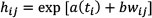
where h_ij and wj are the values of h(t,) and w(t,) on the j^th simulation for the i^th time step. To match survival probabilities, Equations 10 and 12 are combined such that:

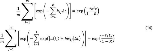
for a total of m simulation trials and k time steps.

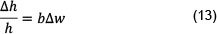
The data required to estimate b effectively (the slope of the regression generated from Equation 14) were procured from South African banks spanning 10 years from January 2003 to January 2013. Combining Equations 10 and 13, the percentage change in spreads may be used as a proxy for percentage changes in hazard rates. i.e.Δs/s = Δh/h. Credit spreads as well as associated change in portfolio value, Δw were assembled for different counterparties of various credit rating grades, and for differing contract maturities. Linear regression of these quantities is shown in Figure 11 (Aw in R000s).

 

 

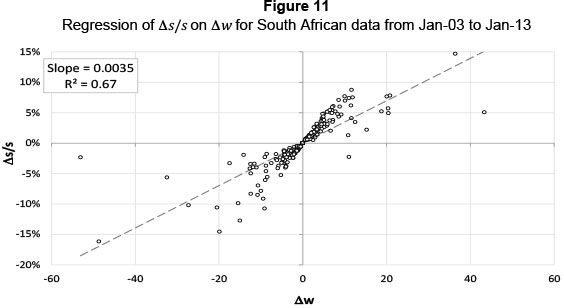
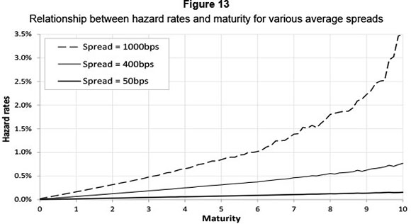
The slope is an estimate for b in the South African market (0.0035 ± 0.0002 with 95 per cent confidence). This value of b is then substituted into Equation 14 and a for each simulation trial determined via a Newton-Raphson technique. Having established a, true hazard rates can be backed out from Equation 14. These are shown in Figure 12 for varying maturities and spreads. The recovery rate was again assumed to be 55 per cent.

 

 

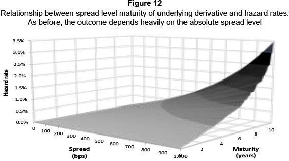
As expected, when spreads are high, hazard rates increase exponentially for longer matureties, as shown in Figure 13.

 

 

5 Conclusions

A step-by-step guide for measuring CVA has been established for a simple OTC interest rate derivative. Implementation of CVA and its associated sensitivity measures for a portfolio of derivative instruments is considerably more complex. Much of this complexity is, however, computational rather than analytical so successful execution involves more computing time rather than calculation difficulties.

CVA risk, which arises from changes in both counterparty credit spreads and market variables that affect the no-default value of derivative transactions, was also explored in detail. CVA is a complex derivative, so it is difficult to estimate the effects of these changes on CVA without a robust mathematical model. High average spreads manifest in times of high market volatility, or in counterparties of poor credit quality, affect CVA risk in counterintuitive (and potentially dangerous) ways. These high spread levels have been observed in South Africa and, although relatively rare, are not impossible. Although there may be an economic justify-cation for the behaviour of CVA when spreads are high, care must be taken not to install complex models blindly without understanding model outputs while considerably more testing is required before market implementation.

It has been demonstrated that a relationship between hazard rates and other observable variables may be modelled and that these models are simpler, computationally faster, and easier to back test than more complex models that have appeared in the literature to date. The model proposed by Hull & White (2012) has been used to calibrate South African data in stressed and unstressed market conditions. Further research is needed to determine which variables work best and to determine the appropriate functional form for the relationship.

 

References

ALOGRITHMICS, 2012. Credit value adjustment and the changing environment for pricing and managing counterparty risk. Available at: www.cvacentral.com/sites/default/files/Algo-WP1209-CVASurvey.pdf [accessed 31-01-2014].         [ Links ]

ASSEFA, S., BIELECKI, T.R., CRÉPEY, S. & JEANBLANC, M. 2009. CVA computation for counterparty risk assessment in credit portfolios, in Recent advancements in theory and practice of credit derivatives, Bloomberg Press:1-27. Available at: http://grozny.maths.univ-evry.fr/pages_perso/crepey/papers/I-C-3.pdf.         [ Links ] [accessed 19-10-2012].

BAILY, M.N. LITAN, R.E. & JOHNSON, M.S. 2008. The origins of the financial crisis, The initiative on business and public policy: Fixing Finance series, Paper 3: November.         [ Links ]

BCBS. 2006. International convergence of capital measurement and and capital standards. Available at: BCBS: www.bis.org/publ/bcbs128.pdf [accessed 19-06-2011].         [ Links ]

BCBS, 2009. Strengthening the resilience of the banking sector. Available at BCBS: http://www.bis.org/publ/bcbs164.pdf [accessed 24-06-2011].         [ Links ]

BCBS, 2011. Basel III: A global regulatory framework for more resilient banks and banking systems. Available at: BCBS: www.bis.org/publ/bcbs189.pdf [accessed 24-06-2011].         [ Links ]

BRENNER, R.J., HARJES, R.H. & KNONER, K.F. 1996. Another look at models of the short term interest rate. The Journal of Financial and Quantitative Analysis, 31(1):85-107.         [ Links ]

BRIGO, D. & CAPPONI, A. 2008. Bilateral counterparty risk valuation with stochastic dynamical models and application to Credit Default Swaps, Working Paper.         [ Links ]

CANABARRO, E. & DUFFIE, D. 2003. Measuring and marking counterparty risk. Chapter 9 in Asset/ liability management for financial institutions, Leo Tilman (ed.): New York.         [ Links ]

CARLSON, J. & SILÉN, A. 2012. Credit value adjustment: risk capital charge under Basel II, Masters thesis, Lund University, Centre for Mathematical Sciences. Available at: http://lup.lub.lu.se/luur/download?func=downloadFile&recordOId=2856020&fileOId=2856025 [accessed 22-10-2012].         [ Links ]

CEPEDES, J.C G., De Juan Herrero, J.A., Rosen, D. & Saunders, D., 2010. Effective modeling of wrong way risk, counterparty credit risk capital and alpha in Basel II. Journal of Risk Model Validation, 4(1):71-98.         [ Links ]

DE PRISCO, B. & ROSEN, D. 2005. Modelling stochastic counterparty credit exposures for derivatives portfolios, Chapter 1 of Counterparty credit risk modelling: Risk management, pricing and regulation, Pykhtin, M. (ed.) Risk Books: London.         [ Links ]

DIEBOLD, F.X. & Li, C. 2006. Forecasting the term structure of government bond yields. Journal of Econometrics, 130(2):337-364.         [ Links ]

FASB (Financial Accounting Standards Board). 2006. Statement of financial accounting standards, No. 157.         [ Links ]

GIBSON, M. 2005. Measuring counterparty credit exposure to a margined counterparty. Chapter 2 of Counterparty credit risk modelling: Risk management, pricing and regulation, Pykhtin, M. (ed.) Risk Books: London.         [ Links ]

GREGORY, J. 2009a. Being two-faced over counterparty risk, Risk, February.         [ Links ]

GREGORY, J. 2009b. Counterparty credit risk: The new challenge for financial markets. Chichester, UK: John Wiley and Sons.         [ Links ]

GROUP OF 20. 2009. Leaders' statement: The Pittsburgh summit. Available at: G20: http://www.pittsburghsummit.gov/mediacenter/129639.htm [accessed 18-12-2012].         [ Links ]

HONG, Y., LI, H. & ZHAO, F. 2004. Out-of-sample performance of discrete-time spot interest rate models. Journal of Business and Economic Statistics, 22(4):457-473.         [ Links ]

HULL, J. & WHITE, A. 1990. Pricing interest rate derivative securities. The Review of Financial Studies, 3(4):573-392.         [ Links ]

HULL, J. & WHITE, A. 1995. The impact of default risk on the prices of options and other derivative securities. Journal of Banking and Finance, 19(2):299-322.         [ Links ]

HULL, J. & WHITE, A. 2012. CVA and wrong way risk. Financial Analysts Journal, 68(5):58-69.         [ Links ]

HULL, J., NELKEN, I. & WHITE, A. 2004. Merton's model, credit risk and volatility skews. Journal of Credit Risk, 1(1):3-28.         [ Links ]

JAMES, J. & WEBBER, N. 2004. Interest rate modelling. Chichester, UK: John Wiley & Sons.         [ Links ]

LAURENT, M.P. 2004. Asset return correlation in Basel II: Implications for credit risk management, Université Libre de Bruxelles, Solvay Business School, Centre Emile Bernheim, Working Papers CEB. Available at: http://www.solvay.edu/EN/Research/Bernheim/documents/wp04017.pdf [accessed 28-05-2013].         [ Links ]

LIPTON, A. & SEPP, A. 2009. Credit value adjustment for credit default swaps via the structural default model. Journal of Credit Risk, 5(2):123-146.         [ Links ]

MAMON, R. S. 2004. Three ways to solve for bond prices in the Vasicek model. Journal of Applied Mathematics and Decision Sciences, 8(1):1-14.         [ Links ]

PYKHTIN, M. & ZHU, S. 2007. A guide to modeling counterparty credit risk. GARP Risk Review, July/August: 16-22.         [ Links ]

REDON, C. 2006. Wrong way risk modeling. Risk, April.         [ Links ]

ROSEN, D. & SAUNDERS, D. 2012. CVA the wrong way. Journal of Risk Management in Financial Institutions, 5(3):252-272.         [ Links ]

SHIMIZU, Y. & YOSHIDA, N. 2006. Estimation of parameters for diffusion processes with jumps from discrete observations. Statistical Inference for Stochastic Processes, 9(3):227-277.         [ Links ]

SOKOL, A. 2010. A practical guide to Monte Carlo CVA. Chapter 14 in Lessons from the crisis, Berd, A. (ed.) London: Risk Books.         [ Links ]

VASICEK, O.A. 1977. An equilibrium characterization of the term structure. Journal of Financial Economics, 5(2):177-188.         [ Links ]

WOOD, D. 2013. Special report: South Africa. Risk Special Report. Available at: http://www.risk.net/risk-magazine/special/2251551/special-report-south-africa [accessed 10-05-2013].         [ Links ]

 

 

Accepted: April 2014

 

 

Endnotes
1 Several banks consider these Basel III proposals to be inadequate and have developed sophisticated, internal models for managing both types of risk (Hull & White, 2012).
2 The Merton model assesses credit risk of a company by characterising the company's equity as a call option on its assets. Put-call parity is then used to price the value of the put and this is treated as an analogous representation of the company's credit risk (Hull et al., 2004)
3 The Johannesburg Securities Exchange implemented a domestic CCP at the end of 2013 (Wood, 2013).
4 is assumption is true when a payment is made at the end of the fixing period - similar to FRNs.
5 For senior unsecured claims, the LGD is 45 per cent (BCBS, 2006) leaving a recovery rate of 55 per cent.
6 99.9 per cent under Basel II rules.