ARTICLES

 

Interpolating yield curve data in a manner that ensures positive and continuous forward curves

 

 

Paul F du Preez^I; Eben Maré^II

^IJohannesburg Stock Exchange
^IIDepartment of Mathematics and Applied Mathematics, University of Pretoria

 

 

---

ABSTRACT

This paper presents a method for interpolating yield curve data in a manner that ensures positive and continuous forward curves. As shown by Hagan and West (2006), traditional interpolation methods suffer from problems: they posit unreasonable expectations, or are not necessarily arbitrage-free. The method presented in this paper, which we refer to as the "monotone preserving r(t)t method", stems from the work done in the field of shape preserving cubic Hermite interpolation, by authors such as Akima (1970), de Boor and Swartz (1977), and Fritsch and Carlson (1980). In particular, the monotone preserving r(t)t method applies shape preserving cubic Hermite interpolation to the log capitalisation function. We present some examples of South African swap and bond curves obtained under the monotone preserving r(t)t method.

Key words: yield curves, monotone preserving cubic Hermite interpolation, positive forward rate curves, South African swap curve

JEL: C650, E400, G120, 190

---

 

 

1 Introduction

A yield curve is a plot depicting the spot rate of interest for a continuum of maturities, in some time interval. Yield curves have a number of roles to perform in the functioning of a debt capital market, including:

1) Valuation of future cash flows;

2) Calibration of risk-metrics;

3) Calculation of hedge ratios; and

4) Projection of future cash flows. Akima (1970)

As noted by Andersen (2007) only a limited number of fixed income securities trade in practice, very few of which are zero-coupon bonds. As such, a model is required to interpolate between adjacent maturities of observable securities, and to extract spot rates from more complicated securities such as coupon bonds, swaps, and Forward Rate Agreements (FRAs). As noted by the Bank For International Settlements (2005), such models can broadly be categorised as parametric or spline-based models.

Under parametric models, the entire yield curve is explained through a single parametric function, with the parameters typically estimated through the use of some least-squares regression technique. Important contributions in this field have come from Nelson and Siegel (1987) and Svensson (1992). As noted by Andersen (2007) the resulting fit of such parametric functions to observed security prices is typically too loose for mark-to-market purposes, and may result in highly unstable term structure estimates. As such, financial institutions involved in the trading of fixed income securities rarely rely on parametric models.

Under spline-based models, the yield curve is made up of piecewise polynomials, where the individual segments are joined together continuously at specific points in time (called knot points). Such methods involve selecting a set of knot points, extracting the corresponding set of spot rates, and finally interpolating in order to obtain a spot rate function. McCulloch (1971) was the first article to suggest modelling the yield curve in such a fashion.

Various methods exist for extracting the set of zero-coupon spot rates corresponding to the chosen set of knot points. Typically, a multivariate optimisation routine is employed whereby the objective is to establish the set of spot rates, which, when combined with an appropriate method of interpolation, produces a yield curve that minimises pricing errors. Such methods have been proposed by McCulloch (1971), McCulloch (1975), Vasicek (1977), Fisher, Nychka and Zervos (1995), Waggoner (1997) and Tangaard (1997). The problem with this type of approach, however, is that the resulting yield curve is rarely capable of exactly pricing back all of its inputs.

Hagan and West (2006) describe an alternative procedure for extracting the set of spot rates which corresponds to the chosen set of knot points. These authors describe a process called bootstrapping, whereby:

1) The set of knot points are chosen to correspond to the maturity dates of the set of input instruments.

2) The set spot rates which correspond to the set of knot points are found via a simple iterative technique.

The abovementioned iterative procedure will converge to a set of spot rates, which, when combined with a chosen method of interpolation, will produce a curve that exactly prices back all input securities. This bootstrap is a generalisation of the iterative bootstrap discussed in Smit (2000). The process of bootstrapping, however, was first described in Fama and Bliss (1987).

Regardless of how the spot rates corresponding to the chosen set of knot points are extracted, careful consideration has to be given to the chosen method of interpolation. Some methods result in discontinuities in the forward curve whilst others are incapable of ensuring a strictly decreasing curve of discount factors (see Hagan & West, 2006). Both scenarios are unacceptable in a practical framework. Discontinuities in the forward curve imply implausible expectations about future short term interest rates (unless the discontinuities occur on or around meetings of monetary authorities), whilst a non-decreasing curve of discount factors implies arbitrage opportunities.

Hagan and West (2006) introduce the monotone convex method of interpolation, and show that this method is capable of ensuring positive, and mostly continuous forward curves. The monotone convex method does, however, under certain circumstances, produce forward curves with material discontinuities. In this paper, we present a method for interpolating yield curve data in a manner that ensures positive and continuous forward curves.

The objective of this paper is not to introduce a "perfect" method for interpolating yield curve data (in fact, our opinion is that such a method does not exist), but rather to present a method that practitioners can use when they require forward curves that are both positive and continuous. To our knowledge, the method presented in this paper is the only method capable of achieving this feat.

 

2 Arbitrage-free interpolation

In an effort to be consistent with the notation of Hagan and West (2006), we define:

• Z(t0, t); the price at time t₀, of the zerocoupon bond maturing at time t.
• r(t₀, t); the continuously compounded spot rate of interest, applicable from time to time .
• f(t₀, t); the instantaneous forward rate, as observed at time , applicable to time .

For ease of notation and without loss of generality, we will assume for the remainder of this paper that t0 = 0, and omit the t₀ term from the abovementioned notation.

The functions Z(t), r(t) and f (t) are related through the following equations:

and

Equations (1) and (2) imply that if f (t) for some t ϵ [0, ∞), then Z (t) is not monotone decreasing at t. If Z (t) is not monotone decreasing, then an arbitrage opportunity must exist. In order to prove this statement, consider the scenario where Z (t₁) < Z (t₂), for t₁ < t₂.

Under such circumstances, and investor would be able to buy a zero-coupon bond maturing at time t₁, and simultaneously sell a zero-coupon bond maturing at time t₂, for an immediate profit of Z.(t₂) - Z (t₁). At time t₁ the investor would simply place the received unit of currency under his/her mattress, and pay it to the buyer of the t₂ bond at t₂.

Note, if represents the price of an inflation-linked zero-coupon bond maturing at t, then the abovementioned arbitrage relation would not necessarily hold. Under such circumstances the cash inflows and outflows at and are not known in advance, seeing that they are inflation dependant. Hence, the cash inflow of (t₂) - Z (t₁) at t₀ would not necessarily constitute a profit.

When interpolating a set of rates that are arbitrage free (in the sense that the input set of discount factors are monotone decreasing), it is crucial that our interpolation function preserve this property.

 

3 Continuous forward curves

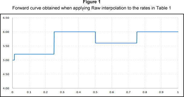
McCulloch and Kochin (2000) point out that "a discontinuous forward curve implies either implausible expectations about future short-term interest rates, or implausible expectations about holding period returns". Considering the zero rates in Table 1; Figure 1 shows the forward curve obtained when applying linear interpolation on the log discount factors (Hagan & West, 2006 refer to this method of interpolation as the "Raw" method).

 

 

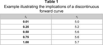
Figure 1 can be interpreted as the curve that depicts the evolution of overnight deposit rates under the term structure given in Table 1. Along the entire curve, overnight rates are seen to jump at each of the knot points used to construct the curve. Clearly, this type of behaviour is implausible, and as such, we should avoid using such curves to value derivative instruments (especially instruments that rely on forward curves to project future cash flows).

When interpolating yield curve data, we would thus prefer to obtain a continuous forward curve (see, for example, Filipovic (2009) and James and Webber (2000) who also note that consistency with a dynamic term structure model is a desirable feature).

 

4 The basic interpolation function

Consider the set of rates r₁, r₂, ..., r_n  for maturities t₁, t₂, ..., t_n. When interpolating, we wish to establish a yield curve function r (t) , for t ϵ [t₁, ... ,t_n], with the following properties:

1) r (t) should interpolate the data in the sense that r (ti) = r_i, for i ϵ {1,2, ..., n}.

2) r (t)should be continuous.

3) In order to present arbitrage potential, the log capitalisation function should be monotone increasing (a monotone increasing capitalisation function implies a monotone decreasing discount function). This property should be relaxed when working with real rates.

4) The forward rate function f(t), for t £ [0, t_n], should be continuous.

We postulate applying a shape preserving cubic Hermite method of interpolation to the log capitalisation function. For the remainder of this paper, we will refer to this method as the "monotone preserving r(t)t" method. Consider the interpolant:

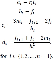
for t_i< t < t_i+1, and define h_i:= t_i+1 - t_i, and m_i := (r_i+1t_i+1 - r_it_i)/h_i.

Suppose the instantaneous set of forward rates f₁, f₂, ..., f_n for maturities t₁, t₂, ..., t_n is known a priori, and relax any arbitrage-free requirements (for the moment). It can then easily be shown (see Hagan and West (2006)) that:

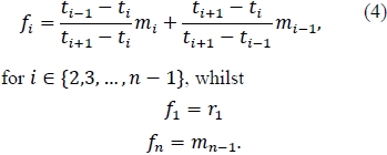
The problem we face in practice is that the instantaneous forward rates are seldom observable. We will thus have to rely on an estimation method, and for this purpose, we postulate using a similar method to that proposed by Hagan and West (2006). We propose estimating f_i, for i ϵ {2,3, ... , n-1}, as the slope at , of the quadratic that passes through the point (t_i-j,m_i-j-1), for j = 1,0,-1. The instantaneous forward rates at the end points, i.e. f₁ and f_n are chosen so as to ensure that f'_{1 =}f'_n = 0.

The instantaneous forward rates are thus estimated as:

 

5 The monotonicity region

We now impose the condition that the log capitalisation function r (t) t be monotone increasing. A monotone increasing function implies a positive forward curve (see equation 2). The work done in the field of shape preserving cubic Hermite interpolation, by authors such as Akima (1970), de Boor and

Swartz (1977), Fritsch and Carlson (1980) and Hyman (1983) suggest amending the estimates for f_i , for i ϵ {1,2, ... n }. In particular, Hyman (1983) notes a simple generalisation of what was recognised by de Boor & Swartz (1977), namely that if r (t) t is locally increasing at t_i, and if:

then r (t) t will be monotone on the interval [ti, ti₊₁], for i ϵ {1,2, ... n-1}. Fritsch and Carlson (1980) independently developed the same monotonicity condition. We will enforce equation (5) in order to ensure that r (t) t is monotone increasing.

We will use the analysis developed by Fritsch and Carlson (1980) to prove the monotonicity region for r (t) t, for t ϵ [0, t_n].

Assume that mi_-1, fi > 0, for i = 1,2, ..., n. Equation (3) implies that:

for t_i< t < ti+₁, , whilst f'(t) is given by:

In order to establish the monotonicity condition implied by equation (5), we need to distinguish between three distinct scenarios:

1) fi + fi₊₁ - 2mi = 0. Here f(t) is a straight line connecting the points f_i and fi₊₁. Since fi, fi₊₁> 0, we observe that f(t) > 0, for t ϵ [ti, ti₊₁].

2) fi + fi₊₁ - 2mi < 0. Here f(t) is a parabola which is concave down, implying that:

for t ϵ [ti, ti₊₁].

3) fi + fi₊₁ - 2mi > 0. Here f(t) is a parabola which is concave up, i.e. f(t) has a unique minimum on the interval [t_i, ti₊₁], for t ϵ [ti, ti₊₁] . Since f_i, f_i+1 > 0 , it follows that if this unique minimum is greater than zero, then f (t) > 0, for tϵ [ti, ti₊₁].

The scenario where fi + fi₊₁ - 2mi > 0 requires further analysis. In particular, observe that under this scenario, f(t) has a local minimum at:

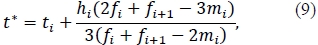
and the value of at is given by:

The function r(t)t will thus be monotone increasing on the interval [ti, ti₊₁], if one of the following conditions is satisfied:

1) t^* < t, or t^* > t .

2) f(t^*) > 0.

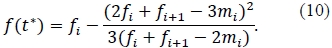
Fritsch and Carlson (1980) define αi = fi/mi, and βi = fi₊₁/mi, from where t* and f(t*) can be written as:

and

where

Note, the condition fi+ fi₊₁ - 2mi > 0 (i.e. the condition under investigation) is equivalent to the condition αi βi - 3 < 0. Equation (11) implies that t^*< t when:

Similarly, t^* > t when:

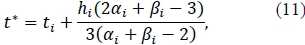
which is equivalent to requiring that αi + 2β_i - 3 < 0. Since m_i > 0, equation (12) implies that f(t*) > 0 when:

It follows that r(t)t will be monotone increasing on the interval [ti, ti₊₁], if one of the following conditions is satisfied:

1) α_i + 2β_i - 3 < 0

2) 2α_i + β_i - 3 < 0

3) Φ(α_ί,β_ί) > 0

4) α_i+β_i -2< 0.

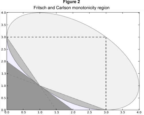
The final condition stems from the fact that f(t) > 0 when f_i + fi₊₁ - 2m_i< 0, as established earlier. Note, Φ (α_{ί,βi) = 0 is the ellipse described by:}

The abovementioned monotonicity constraints are graphically illustrated in Figure 2. The shaded areas represent the areas where r (t) t will be monotone increasing. The area bounded by the α and β axis, and the dotted lines at α = 3 and β = 3 represents the de Boor and Swartz (1977) monotonicity region. This region implies that if α_i,β_i < 3, then r(t)t will be monotone increasing.

 

 

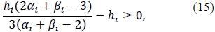
Requiring that is equivalent to requiring that fi, fi₊₁< 3, and can be achieved by requiring that:

for i ϵ {2, 3, ... n - 1}. In order to ensure that the function r (t) t, for t ϵ [t₂, t_n-1] is monotone increasing, we can thus clamp fi as follows:

for i ϵ {2,3, ... n -1}. Note, f(t) will be positive on the interval [t₁, t₂] provided:

and similarly f(t), will be positive on the interval [tn_-1', t_n] provided:

Since f₁= m₁, and fn = mn_-1 , the clamping proposed by equation (19) will ensure that r (t) t is monotone increasing, for t ϵ [t₁,t_n].

If negative forward rates are allowed, i.e. when considering inflation-linked yield curve data, we will simply omit the clamping proposed by equation (19).

 

6 Extrapolation

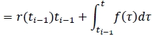
From equation (2) it follows that:

which implies that if t ϵ [ti_-1, t_i], then:

A simple (and naive) method of extrapolation is obtained by assuming that f (t) is constant before t₁ and after tn . More specifically, we will require that f (t) = f₁ when t < t₁, and we will require that f(t) = fn , when t > tn.

Equation (21) implies that:

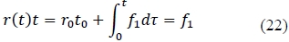
when t < t₁, whilst:

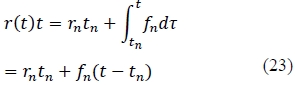
when t > tn. Note, the abovementioned method of extrapolation was specifically chosen to ensure continuity in r(t) and f(t), at t₁ and

 

7 Locality

If we change the value of an input at ti, then we would like to know the interval [ti_-l, ti+u], on which the interpolated yield curve values change. Hagan and West (2006) define l and u as locality indices, and use them to determine the degree to which an interpolation algorithm is local.

Changing the value of ri would clearly affect the values of mi_-1 and mi. It follows from equation (6) that changing the value of mi_-1 would affect the values of fi and fi_-1 , whilst changing the value of mi would affect the values of fi and fi₊₁. Changing the value of ri thus affects the values of fi_-1, fi, and fi₊₁, which in turn affects the coefficients ci_-2, ci_-1, ci and ci₊₁. The value of r (t) will thus be affected on the interval [ti_-2, ti₊₂]. It follows that the monotone preserving r (t)t method has locality indices l = u = 2.

 

8 Results

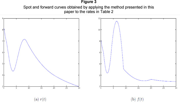
Hagan and West (2006) use the rates given in Table 2 to illustrate the inadequacies of various methods of interpolation. The input set of discount factors are monotone decreasing, and the interpolated curve should preserve this property.

 

 

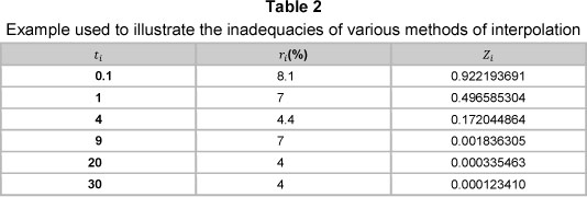
Figure 3 shows the spot and forward curves obtained by applying the monotone preserving r (t) t method to the rates in Table 2. The resulting forward curve is positive and continuous, a feat not be taken lightly; the monotone convex method is the only other method that achieves this feat for this particular example.

8.1 Monotonicity vs. continuity

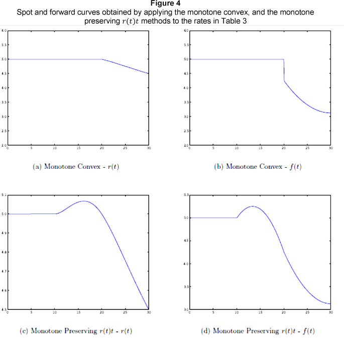
The method presented in this paper aims to ensure a positive and continuous forward curve, however, under certain circumstances, continuity is ensured at the expense of monotonicity. Consider the rates in Table 3, Figure 4 shows the corresponding spot and forward curves obtained by applying the monotone convex method, and monotone preserving r (t) t method.

 

 

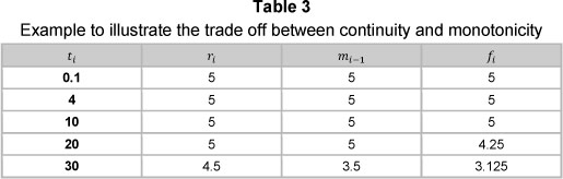
Figure 4 highlights the weaknesses of both methods:

1) Under the monotone convex method, f (t) is seen to have a material discontinuity at t = 20.

2) Under the monotone preserving r (t) t method, both r (t) and are increasing in the to year region, and then decreasing in the to year region. This behaviour is somewhat unintuitive; the input data suggests that both r (t) and f (t) should be constant in the 10 to 20 year region.

Figure 4 shows that under the monotone convex method, monotonicity trumps continuity, whilst the converse is true for the monotone preserving r (t) t method. When deciding on an appropriate method to interpolate yield curve data, the user has to decide what is more important for his/her particular purpose; monotonicity or continuity. Different users will have different criteria.

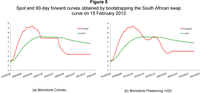
8.2 The South African swap curve

Figure 5 is an example that illustrates the spot and 90-day forward curves obtained by bootstrapping the South African swap curve under the monotone convex, and the monotone preserving r (t) t methods.

For this particular example, the spot and forward curves produced by the monotone convex, and the monotone preserving r (t) t methods are seen to be remarkably similar. The fundamental difference between the two methods is, however, clearly illustrated:

1) under the monotone preserving r (t) method, the forward curve is a set of parabolas joined together in a continuous fashion, whilst

2) under the monotone convex method, the forward curve is also a set of parabolas, however, if on a specific segment, the monotonicity of the input data is compromised, the parabola is augmented (which can lead to discontinuities, as seen earlier).

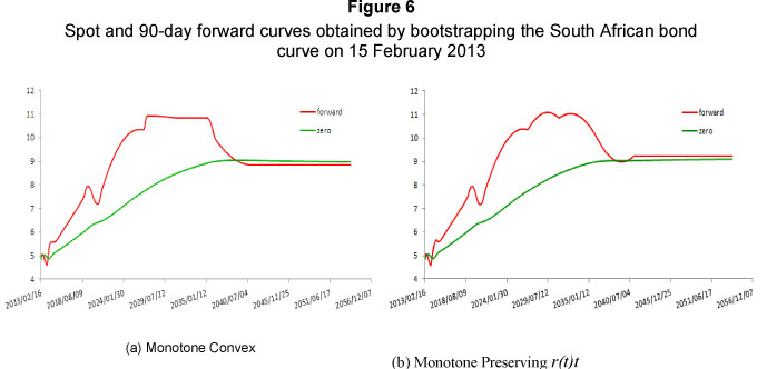
8.3 The South African bond curve

Figure 6 is an example that illustrates the spot and 90-day forward curves obtained by bootstrapping the South African bond curve under the monotone convex, and the monotone preserving r (t) t methods. Again, the fundamental difference between the two methods is clearly illustrated.

 

9 Conclusion

In this paper, we presented a method for interpolating yield curve data in a manner that ensures positive and continuous forward curves (the monotone preserving r (t) t method). Positive forward curves are essential from an arbitrage-free perspective, whilst discontinuous forward curves imply implausible expectation about future short term interest rates.

The monotone preserving r (t) t exhibits some weaknesses: the forward curve is continuous but there are points of non-differentiability (differentiable forward curves are often required to calibrate no-arbitrage term structure models, like the models of Ho & Lee (1986); Hull & White (1990); Cox, Ingersol & Ross (1985)), and under certain conditions, continuity in the forward curve is preserved by sacrificing monotonicity in the forward curve. However, when interpolating yield curve data, all methods exhibit weaknesses; traditional methods either imply discontinuous forward curves, or they fail to ensure positive forward curves (sometimes both).

The aim of this paper was not to introduce a "perfect" method for interpolating yield curve data, but rather to present a method that practitioners can add to their arsenal when interpolating yield curve data. The onus is then on the practitioner to define the properties which he deems to be the most important, and to then apply the appropriate interpolation method.

 

Acknowledgement

The authors wish to express their gratitude towards the anonymous referees whose views and comments aided in the presentation of this article.

 

References

BANK FOR INTERNATIONAL SETTLEMENTS. 2005. Zero-coupon yield curves: Technical documentation. BIS Working Papers, 25.         [ Links ]

AKIMA, H. 1970. A new method of interpolation and smooth curve fitting based on local procedures. Journal of the Association for Computing Machinery, 17(4):589-602.         [ Links ]

ANDERSEN, L. 2007. Discount curve construction with tension splines. Review of Derivatives Research, 10(3):227-267.         [ Links ]

COX, J.C., INGERSOL, L.J. & ROSS, S.A. 1985. A theory of the term structure of interest rates. Econometrica, 21(4):385-407.         [ Links ]

DE BOOR, C. & SWARTZ, B. 1977. Piecewise monotone interpolation. Journal of Approximation Theory, 21(4):411-416.         [ Links ]

FAMA, E. & BLISS, R. 1987. The information in long-maturity forward rates. The American Economic Review, 7(4):680-692.         [ Links ]

FILIPOVIC, D. 2009. Term-structure models: A graduate course. Springer Finance.         [ Links ]

FISHER, M., NYCHKA, D. & ZERVOS, D. 1995. Fitting the term structure of interest rates with smoothing splines. Federal Reserve System Working Paper # 95-1 .         [ Links ]

FRITSCH, F.N. & CARLSON, R.E. 1980. Monotone piecewise cubic interpolation. SIAM Journal of Numerical Analysis, 17(2):238-246.         [ Links ]

HAGAN, P.S. & WEST, G. 2006. Interpolation methods for curve construction. Applied Mathematical Finance, 13(2):89-129.         [ Links ]

HAGAN, P.S. & WEST, G. 2008. Methods for constructing a yield curve. Wilmott Magazine, May, 70-81.         [ Links ]

HO, T. & LEE, S. 1986. Term structure movements and pricing interest rate contingent claims. Journal of Finance, 41(5):1011-1029.         [ Links ]

HULL, J. & WHITE, A. 1990. Pricing interest rate derivative securities. The Review of Financial Studies, 3(4):573-592.         [ Links ]

HYMAN, J.M. 1983. Accurate monotonicity preserving cubic interpolation. Journal on Scientific and Statistical Computing, 4(4):645-654.         [ Links ]

JAMES, J. & WEBBER, N. 2000. Interest rate modeling. Wiley & Sons.         [ Links ]

MCCULLOCH, J.H. 1971. Measuring the term structure of interest rates. Journal of Business, 44(1):19-31.         [ Links ]

MCCULLOCH, J.H. 1975. The tax adjusted yield curve. Journal of Finance, 30(3):811-830.         [ Links ]

MCCULLOCH, J.H. & KOCHIN, L.A. 2000. The inflation premium implicit in the US real and nominal term structures of interest rates. Technical report, Ohio State University (Economics Department), 12.         [ Links ]

NELSON, C.R. & SIEGEL, A.F. 1987. Parsimonious modelling of yield curves. Journal of Business, 60(4):173-489.         [ Links ]

SMIT, L. 2000. An analysis of the term strucure of interest rates and bond options in the South African capital market. PhD Thesis, University of Pretoria .         [ Links ]

SVENSSON, L.E. 1992. Estimating and interpreting forward interest rates: Sweden 1992-1994. NBER Working Paper, 4871.         [ Links ]

TANGAARD, C. 1997. Nonparametric smoothing of yield curves. Review of Quantitative Finance and Accounting, 9(3):251-267.         [ Links ]

VASICEK, O.A. 1977. An equilibrium characterisation of the term structure. Journal of Financial Economics, 5(2):177-188.         [ Links ]

WAGGONER, D.F. 1997. Spline methods for extracting interest rate curves from coupon bond prices. Federal Reserve Bank of Atlanta Working Paper, 10.         [ Links ]

 

 

Accepted: March 2013

 

 

To a large extent, this paper is motivated by the work of Patrick Hagan and Graeme West (see Hagan & West, 2006; Hagan & West, 2008)). As a sign of appreciation, we would like to dedicate this paper to the memory of Graeme West.