


Servicios Personalizados
Articulo
 Inglés (pdf)
 Articulo en XML
 Referencias del artículo
Indicadores

Links relacionados
-
 Citado por Google
 -
 Similares en Google
Compartir

 Permalink
South African Journal of Economic and Management Sciences
versión On-line ISSN 2222-3436
versión impresa ISSN 1015-8812
S. Afr. j. econ. manag. sci. vol.16 no.4 Pretoria ene. 2013
ARTICLES
Empirical analysis of space and capital markets in South Africa: A review of the REEFM - and FDW models
Douw GB Boshoff
Department of Construction Economics, University of Pretoria
ABSTRACT
This paper assesses the different models, in conjunction with the different theories surrounding the distinction and interdependencies between space- and capital markets. First, the theory of space- and capital markets is discussed with reference to two models, the FDW and the REEFM models. The FDW model provides a diagrammatic explanation of the behaviour of the property market, while the REEFM is an econometric model based on statistical principles that are able to forecast property-market behaviour by interpreting specific given variables. The REEFM model as the perceived more sophisticated model, untested in South Africa, was then analysed to test its applicability in the South African context. The findings confirmed the applicability of the model, although one part is not confirmed and is suggested for further research.
Key words: FDW model, REEFM model, property economics, property market behaviour
JEL: G140, 170, 100, 190, P470
1 Background
The unique characteristics of real estate create, on the one hand, many opportunities for real estate investors, and, on the other, many difficulties. The different factors influencing the behaviour of real estate should therefore be investigated carefully.
DiPasquale and Wheaton (1992:181) stated that analysing the market for real estate presents challenges because of the interrelation of space- and asset markets.
The earliest recording of work that distinguishes between use decisions and investment decisions with respect to real estate was probably Weimer (1966), but Hendershott and Ling (1984) were the first to integrate space-and capital markets into real estate. According to Viezer (1999:504), Hendershott and Ling's model evaluated investment value responses to tax code alterations in a dynamic programming algorithm that used a traditional discounted cash-flow equation with assumed parameters.
Corcoran (1987) graphed the space market and capital market of real estate separately, but interdependently, explicitly distinguishing between the short- and long-run supply of space. A similar model was published by Fisher (1992: 167). Fisher shows the equilibrium existing between the short- and long-run situations of the space and capital markets.
DiPasquale and Wheaton (1992) and Fisher, Hudson-Wilson and Wurtzebach (1993) further refined this model, which is referred to as the diagrammatic model by Viezer (1999:504)). The model was officialized in a textbook on property economics by DiPasquale and Wheaton (1992) as the FDW-model, the most detailed treatment found in a seminal textbook.
Du Toit (2002) carried out research on the FDW-model and describes the principles of the model with an accompanying practical example of office space in Pretoria. The FDW-model conceptualizes the interrelationships between the market for space, asset valuation, construction sector and stock adjustment.
Viezer (1998) developed a completely new model that similarly describes the space and asset markets in the property sector, but this model is of an econometric rather than diagrammatic nature. Viezer refers to it as the Real Estate Econometric Forecast Model (REEFM), and uses statistical principles to explain the property market, in contrast with the diagrammatical FDW-model.
2 Research problem
The literature reviewed shows the development of models that distinguish between space and capital markets in real estate. This appears to be a logical exposition of measuring the activities in the real estate market, with the possibility of explaining the movements in the real estate sector. Although some research could be found on the application of the FDW-model in the South African context, nothing could be found on the application of the REEFM model in South Africa, even though it appears to be more sophisticated, with well-described econometric equations.
The aim of this study is to test the applicability of the REEFM model in the South African context by way of statistical analysis. The different equations specified in the model will be analysed by applying South African data and testing the significance of each equation by diagnostic testing. If each equation in its own right can be confirmed, using the results of all the preceding equations, the model can either be confirmed as applicable or rejected as not applicable to South African data.
The null-hypothesis, that the six stochastic and four deterministic equations of the REEFM model, as proposed in section 4, do not properly explain behaviour in the South African market. If the null-hypothesis can be rejected, then the alternative hypothesis can be accepted that the equations form a meaningful model for explaining behaviour in the South African property market.
3 The FDW model
3.1 The FDW-model defined
Archour-Fischer (1999:33) states that the Fischer-DiPasquale-Wheaton model is an elegant metaphor that integrates the different markets in the built environment, with specific reference to the property market, the capital market and construction activity. Du Toit (2002:10) describes the FDW model as being a static quadrant model that has the ability to trace the relationships between real estate market and asset market variables. Archour-Fischer also suggests that it is a dynamic model (Archour-Fischer, 1999:40-42), in which the parameters of the model can be changed to determine the influence in the different markets represented by the model, although Viezer (1998) criticizes the application of the model (see section 2.3).
Taking into consideration the flow of real estate as discussed by DiPasquale and Wheaton, it is evident that the depreciation of real estate and the subsequent replacement of such depreciation is an output of the model, as it is a reduction in the stock level seen in quadrant four of the model. The reduction and replacement cause a shift in the supply and demand patterns so that the market reacts to it. It thus acts as an input to the rest of the model. The model reacts to the changes and further depreciation takes place, resulting in a change in the then present stock level.
A discussion of the theory relating to the model will be presented in the following section. It should, however, be emphasized that Du Toit has already extensively discussed the principles of the model, and it is not the intention of this study to reproduce his work. However, it is necessary to include a detailed discussion of the model in order to explain different concepts later in the article.
Figure 1 shows a graphical illustration of the model, which consists of four quadrants, as shown in Figure 1, and represents the following (Archour-Fischer, 1999:34-37):
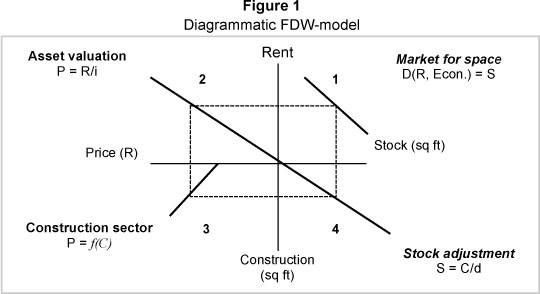
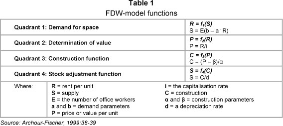
Quadrant 1 - Demand function on the market for space;
Quadrant 2 - The valuation function;
Quadrant 3 - The construction function;
Quadrant 4 - The adjustment supply.
Quadrant 1 indicates the demand function on the market for space demanded by users, represented in this study by the occupiers of office space. With a static supply, the price of space or rent level will increase when demand increases, and conversely. In equilibrium, the supply of property should be equal to the demand at various price levels.
In Quadrant 2 the rent level applicable to the equilibrium level of demand is discounted at the capitalisation rate, which is illustrated in Figure 1 as the slope of the asset valuation curve, to arrive at the asset value, represented by the function P = R/i.
Quadrant 3 represents the construction activity, which is a function of the asset value. When the asset value is higher than construction costs (represented in Figure 1 as the intersection of the construction curve and the x-axis), new F construction will be triggered, otherwise construction will come to a halt. Thus, Ρ = f(C).
The level of construction activity is carried over to Quadrant 4, the adjustment of supply, and is given by the function S = C /d, or ΔS = C-dS.
3.2 Theoretical testing
3.2.1 Assumptions
Some of the information crucial to the calculation of the variables and equilibrium level in the model was not supplied by the author of the literature (Archour-Fischer, 1999). The missing variables were therefore selected as follows:
- Market capitalisation rate (i) - 11 per cent
- The α parameter - 0.01
It should be noted that only the α or the β parameter need be supplied, as the other is then calculated from given data. The value of 0.01 assigned to the α parameter indicates a slope of the construction function of 0.01. This means that the construction activity will change one unit for every hundred units change in the value of space. The β parameter is then calculated as R 1 669.90, which indicates that new construction will be triggered when the value per unit is more than that shown in the figure below.
3.2.2 Calculations
In order to test the validity of the model's functions, the different calculations should indicate an equilibrium level. The first function, the demand for space, determines the supply, according to the given figures. The last function also calculates supply, but from another set of parameters. Therefore, should there be equilibrium, both calculations would result in the same answer.
The calculations are carried out separately for each quadrant, which will indicate how each quadrant is influenced. The last quadrant should end with the same answer as that of the first quadrant.
Quadrant 1: S = E(b - a . R)
= 100 000 office workers (420 - 2 x R 201.78 per worker)
= 100 000 (420 - 403.56)
= 100 000 (16.44)
= 1 644 000 m2
Quadrant 2:
P = R / i
= 201.78 / 0.11
= R 1 834.36
Quadrant 3:
C = (P - β) / α
= (1 834.36 - 1 669.90) / 0.01
= 16 446 m2
Quadrant 4:
S = C / d
= 16 446 / 0.01
= 1 644 600 m2
The results for S above are indicated by 1 644 000 m2 and 1 644 600 m2. This indicates a variance of 0.03%, which is accepted as a result of the approximation of decimals and is statistically within acceptable range.
3.3 Remarks on the FDW model
The FDW model seems to offer an acceptable interpretation of the property market using a diagrammatic model, which is mathematically explained by the developers of the model. However, Viezer (1998) points out that the FDW model is of little value as an investment tool, and he develops a Real Estate Econometric Forecast Model (REEFM) that is able to forecast implicit market returns. The REEFM seems to be of much more value as an investment tool, as it can be used for calculating historical returns and forecasted returns.
According to Archer and Ling (1997), a multi-factor asset pricing model should be used to determine the discount rate, which in turn would determine both the market value and the cap rate, rather than assuming that the cap rate is exogenously determined. Viezer (1998) developed an econometric model for the integration of real estate's space and capital markets - the Real Estate Econometric Forecast Model (REEFM). In his research, he answers the above comment by Archer and Ling by including a stochastic equation for, inter alia, the cap rate. Viezer's equation contains five predetermined variables four of which are taken, with some modifications, from the pre-specified Arbitrage Pricing Theory (APT) model by Chen, Roll and Ross (1986).
The FDW model is interpreted by Viezer (1998) to suggest that equilibrium is a natural state where all values are determined simultaneously, but in reality there are lags in the adjustment process. Viezer (1999:507) also modifies the DiPasquale and Wheaton (1992) model by positing that real construction costs are a function of the lagged net change in stock, rather than a current-period new construction.
Viezer further points out that the FDW model is of little value in terms of practical advice, and is limited to forecasting the changes in the direction of real estate markets and general levels of return. He maintains that the model should be estimated statistically in individual markets if it is to be useful to the practitioner. The REEFM integrates real estate's space and capital markets econometrically rather than diagrammatically. The model also links the short- and long-run markets, and calculates implicit market returns for property markets (Viezer, 1998:143). The model can therefore be used as an effective investment or forecast tool. The only forecast inputs needed are the local economic variables, and national financial variables (Viezer, 1998:144).
4 The REEFM model
4.1 Principles of REEFM
It should be emphasised that it is not the intention of this paper to either explain or to discuss the fundamentals of the REEFM, or to investigate the validity of the research by Viezer (1998). The paper will test only the applicability of the model for use in the South African property market.
The conceptual framework of REEFM is illustrated in Figure 2 (Viezer, 1998:107). REEFM is a recursive model, containing six stochastic equations (occupancy, real rents, capitalisation rate, market value per unit, change in stock, and real construction costs) and seven deterministic equations (a net operating income proxy, market value per unit, stock of space, vacancy rate, implicit appreciation market return, implicit income market return and implicit total market return) (Viezer, 1998:134-5).
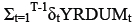
The six stochastic equations given by Viezer are all in the format:
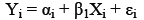
where:
αi = Y intercept for the population;
βl = slope for the population;
εi = random error in Y for observation i.
This relationship is confirmed by two sources, with different formats for the same equation:
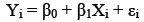
(Levine, Berenson & Stephan, 1998:538) and;

(Steyn, Smit & Du Toit, 1989:378), which is the function of a straight line relationship between x and y.
Each of the stochastic equations is a variation of the above equation, allowing for the different variables that influence the Yi -factor. In all six equations the variable:
is also added, which is missing data indicators to be used in estimating the unbalanced panel (Viezer, 1998:115).
The deterministic equations are in different formats, calculating a specific result in each case by combining the results from the stochastic equations.
In both the stochastic and deterministic equations, the variables are given in the format Vp.m.t., which in this case would indicate a variable (V) for property type p, in metro area m, at time period t.
The different equations will be discussed in the text to follow, and the similarities and differences relating to the FDW model will be explained.
4.1.1 Short-run asset market

(Viezer, 1998:115)

(Viezer, 1998:115)
Viezer explains occupancy (OCCp.m.t.) as a function of lagged real rent, (RNT$p.m.t, nominal rent deflated by the Consumer Price Index) and an economic variable. The economic variable in the case of office space would be office employment. Real rents, in turn, respond with a lag to vacancies in the market (Viezer, 1998:114-15). On the contrary, the FDW model only takes the demand as equal to the supply of office space, using only the equation S = E(b - a.R) to calculate this (see section 2.2.2). Rent levels are taken as a given, and are not calculated as above. This means that the variables are calculated according to a much less scientific method, limiting the capabilities of the model for the historical explanation of the market, as well as possibilities for forecasting, which would be much more useful.
The first deterministic equation is a proxy for the net operating income (NOIp.m.t). The net operating income is determined by multiplying the occupancy by the rental levels. However, the rental levels are calculated for real rent in terms of equation 2 and should therefore be inflated by the Consumer Price Index (CPI). The equation for the net operating income is therefore:

(Viezer, 1998:117)
4.1.2 Short-run capital market
The capital market attempts to translate the results of the short-run space market into asset prices. "The reasonably calculated expected future net income flow of an investment property discounted to its present value, when capitalised at the prevailing rate sought by prudent investors, represents the estimated capitalised value of the property at that time" (SAIV, 1999:6-4). When considering the future income stream, it increases approximately in line with inflation, or the country's CPI. The income stream can therefore be capitalized by dividing the first year's income by the capitalisation rate, which is the discount rate minus CPI. As the discount rate is not determined, the Cap rate cannot be determined from the discount rate. However, Viezer determines the Cap rate with the equation:

(Viezer, 1998:123)
The variable RNTp.m.t.-1/MSFp.m.t.-1 considers the backward-looking comparisons of appraisers and therefore takes into consideration historical data. %ΔECONp.m.t is the percentage change in the economic variable as used in the equation for occupancy. INFLt is the current inflation rate, while RISKt and TERMt are risk variables used by Viezer as the difference between the corporate Baa bond rate and the 10-year Treasury bond rate, and the difference between the 10-year Treasury bond rate and the 3-month Treasury bill rates respectively (Viezer, 1998:123, 124).
With the Cap rate established, it is possible to calculate the market value per unit for the metro property stock with the equation:

(Viezer, 1998:124)
The PASS variable indicates the extent to which the inflation rate is passed through to the property appreciation. The MSFE variable is then regressed to determine the actual property value per unit:

(Viezer, 1998:124)
While the above equations are used to determine the per unit market value of property, the FDW model divides the demand, multiplied by the rate per unit, by the cap rate to get to the market value. While REEFM takes into consideration different risk factors as well as economic variables for calculating the cap rate, the FDW model does not indicate how this is calculated (Du Toit, 2002:31). From this it is also taken that REEFM calculates the market value of property in a much more scientific way, which creates an opportunity for explaining the current market as well as forecasting future trends.
4.1.3 Long-run space market
The long-run space market is the addition of new stock or construction and the removals of stock or depreciation. These construction and removals are a function of the difference in quantities (STK - OCC) and real prices (MSF$ - CST$) (Viezer, 1998:132). The asset market is expressed in quantities and the capital market is expressed in prices with the following equations:
Asset market:

(Viezer, 1998:132)
The stock of space in the current period takes into consideration the stock in the previous period, plus the current period's construction, minus the current period's removals:

(Viezer, 1998:132)
Capital market:

(Viezer, 1998:132)
In the above, the real construction costs are indicated as being a function of the lagged net change in stock (Viezer, 1998: 132).
The last equation to close the loop for the model is the vacancy rate:

(Viezer, 1998:133)
The FDW model is represented as a static model, and does not take into consideration any new construction. Construction is calculated by the FDW model only as the replacement of depreciation. The depreciation rate is given as a set figure (Archour-Fischer, 1999:37). From this it is evident that any influence of the long-run space market on the equilibrium level is excluded from the FDW model, which puts into question the validity of any practical use of the FDW model.
5 Case study
In order to apply the theory to practice, secondary data of macro-economic statistics (South African Reserve Bank, 2013) and infor mation of offices in the property market (Rode, 1990 to 2008) were investigated. Data were captured per quarter for the period from Quarter 1 (1990) to Quarter 3 (2008). The totals were aggregated to a national level, and were substituted into the theoretical model for analysis.
The data is mostly of a time-series nature and for regression purposes is transformed by way of first differences and log-transformation where applicable. Details of transformation and the different data sets that were used are explained in the text.
5.1 Short-run space market
The short-run space market consists of two stochastic and one deterministic equation. The first stochastic equation, OCCt, is a function of real rent and an economic variable as per equation 1.
The economic variable for office type properties is the number of office workers. For the purposes of calculation in this study, the figures for total employment in the private sector are used.
RNT$t levels are a function of the vacancy levels in the preceding period, and could therefore be predicted when the vacancy level is available using equation 2.
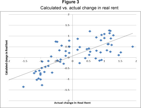
The applicability of preceding-period vacancies to determine real rent is tested by a regression of the actual quarterly rental levels to the actual quarterly vacancy level preceding the current time period with one year in terms of equation 2. The result is an adjusted R square of 0.043 with an f-value of 4.351. The critical f-value is 3.98 and 7.05 at the 0.05 and 0.01 levels respectively. Although the regression rejects the hypothesis that previous-period vacancies cannot explain the variance in real rents, the correlation is negligible. Furthermore, the Durbin-Watson statistic shows a value of 0.212, while dL and dU are 1.583 and 1.641 respectively. This also suggests evidence of autocorrelation. By transforming the data by way of a first difference, the Durbin-Watson statistic changes to 1.524, which just fails to reject the hypothesis that no autocorrelation exists, but the R square changed to -0.014 with an f-value of 0.043. By using annual rather than quarterly data, the adjusted R square increased to 0.649 with an f-value of 28.757. The critical f-value is 8.86 at the 0.01 level, confirming that previous-period vacancies are a good indicator of current period rental levels. The Durbin-Watson statistic for the annual data was determined as 1.543, with dL and du at 0.776 and 1.054 respectively. The hypothesis that autocorrelation is present in the annual data can therefore be rejected. The actual versus the calculated real rent is shown graphically in Figure 3.
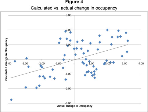
The use of equation 1 to calculate occupancy, revealed that first difference transformed rentals of the preceding-period, in combination with employment data that is also first different transformed, failed to predict occupancy. However, if the first difference of current-period rentals is used, an adjusted R square of 0.360 is determined, with an f-value of 5.50. The critical f-values for the 0.05 and 0.01 levels of significance are 3.74 and 6.51 respectively. It could therefore be accepted with at least 95% confidence that 36% of the variance in the occupancy is explained by current-period rentals and employment.
The Durbin-Watson statistic for the regression is 1.548, with dL and dU for the 0.01 level at 0.66 and 1.254 respectively. The suggestion of any autocorrelation in the data can therefore be rejected. The actual versus the calculated occupancy is illustrated in Figure 4.
5.2 Short-run capital market
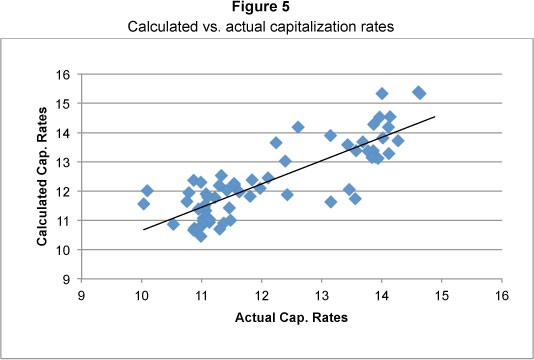
Equation 4 calculates capitalisation rates with reference to bond rates, inflation, changes in employment (South African Reserve Bank, 2013) and previous-term rent/value relationships (Rode, 1990 to 2008). The data has been log transformed for purposes of calculation.
The quarterly data provided reasonably good results, but the Durbin-Watson statistic at 0.328 failed to reject the hypothesis of no autocorrelation. Annual data not only resolved the autocorrelation, but also increased the adjusted R square from 0.366 to 0.634, while the f-value changed from 8.86 to 6.882. The critical f-value for the annual data is 5.06 at the 0.01 level, indicating that equation 3 can largely explain the movement in capitalization rates with 99% confidence. The comparison of actual versus calculated capitalization rates is illustrated in Figure 5.
With the capitalisation rates determined, it is possible to capitalise the NOI, which is determined in terms of equation 3, then to calculate the market value per unit in terms of equation 5. Equation 6 is then used to regress the actual property value per unit. The first difference transformed quarterly data and provided a good fit, but once again the Durbin-Watson statistic at 0.244 failed to reject evidence of no autocorrelation. The annual data provided an adjusted R square of 0.622 with an f-value of 20.744. The critical f-value at the 0.01 level is 9.65. The Durbin-Watson statistic in this case is 1.409, with the dL and dU values at 0.653 and 1.010 at the 0.01 level. It is therefore confirmed that evidence of autocorrelation is rejected. The calculated vs. actual change in MSF values is presented in Figure 6.

5.3 Long-run space market
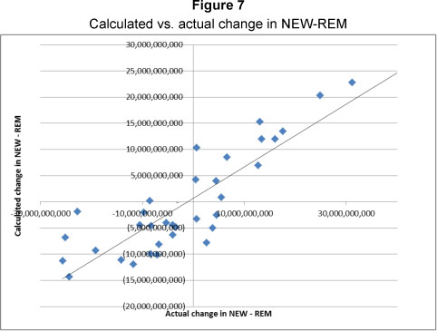
For the asset market, the regression of the first difference of NEW-REM as per equation 7 resulted in an adjusted R square value of 0.553 for the annual data. NEW-REM is taken as the annual change in all fixed assets as reported by the South African Reserve Bank (2013). The f-value is 5.944 with a critical f-value of 5.14 at the 0.05 level. The hypothesis that equation 7 is true could therefore be accepted at the 0.05 level, but failed to reject the null hypothesis that equation 7 is not true at the 0.01 level. The Durbin-Watson statistic obtained a value of 1.804, which confirms that no autocorrelation is present. The comparison of calculated versus actual change in NEW-REM is displayed in Figure 7.
When analysing the capital market, the only equation that failed to provide satisfactory results was the change in construction cost to be a function of the change in stock. By analysing quarterly or annual data the adjusted R square values were 0.20 with the f-values also below 0.20. This indicated that equation 9 failed to reject the hypothesis that construction costs are not affected by previous-period changes in stock. However, this is not considered critical at this stage in order to arrive at a conclusion, but it is recommended that the specific analysis of this be investigated by way of further research.
5 Conclusion
The paper investigated different models that considered the space and capital markets in real estate, testing the applicability of the principle of space and capital market differentiation on the South African property market. Although the theoretical principles of two models, the FDW and REEFM models, were discussed, only the REEFM model was tested empirically for application in the South African context. The different equations that form the REEFM model were tested individually and it was found that all but one equation had statistical significance when explaining office property behaviour. The model as a combination of the set of equations could also be accepted as applicable because the results of each equation were carried forward to the next. The hypothesis at each equation is therefore tested according to the calculated data from all the equations combined. By confirming the applicability of the individual equations, the combined dataset could therefore also be accepted as applicable.
The value of this paper lies in the possibility of applying the model in the South African context in order to monitor property behaviour more closely. It is recommended that the model also be tested on other real estate asset types, i.e. industrial, retail or residential, or to apply the principles on smaller markets, i.e. specific geographical areas. As such it could be used successfully to explain specific property economics, or even to valuate property in general.
References
ARCHOUR-FISCHER, D. 1999. An integrated property market model: A pedagogical tool. Journal of Real Estate Practice and Education, 2(1). [ Links ]
ARCHER, W R & LING, D.C. 1997. The three dimensions of real estate markets: Linking space, capital, and property markets. Real Estate Finance, 14:7-14. [ Links ]
CHEN, N., ROLL, R. & ROSS, S.A. 1986. Economic forces and the stock market, Journal of Business, 59:383-403. [ Links ]
CORCORAN, P.J. 1987. Explaining the commercial real estate market. Journal of Portfolio Management, 13:15-21. [ Links ]
DIPASQUALE, D. & WHEATON, W.C. 1992. The markets for real estate assets & space: A conceptual framework. Journal of the American Real Estate and Urban Economics Association, 20(1):187-97. [ Links ]
DU TOIT, H. 2002. Appraisal of the Fischer-DiPasquale-Wheaton (FDW) real estate model and development of an integrated asset market model (IPAMM). Unpublished treatise submitted in part fulfilment of the requirements for the MSc (Real Estate), University of Pretoria. [ Links ]
FISHER, J.D. 1992. Integrating research on markets for space and capital. Journal of Real Estate and Urban Economics Association, 20(1):161-80. [ Links ]
FISHER, J.D., HUDSON-WILSON, S. & WURTZEBACH, C.H. 1993. Equilibrium in commercial real estate markets: Linking space and capital markets. Journal of Portfolio Management, 19:101-107. [ Links ]
HENDERSHOTT, P H & LING, D C, 1984. Prospective changes in tax law and the value of depreciable real estate. Journal of the American Real Estate and Urban Economics Association, 12:297-317. [ Links ]
LEVINE, D.M., BERENSON, M.L. & STEPHAN, D. 1998. Statistics for managers. New Jersey: Prentice Hall. [ Links ]
RODE & ASSOCIATES. 1997 to 2002. Rode's report on the SA property market. 1990:1 - 2008:3. [ Links ]
SOUTH AFRICAN INSTITUTE OF VALUERS (SAIV). 1999. The valuers' manual. (7th ed.) Durban: Butterworths. [ Links ]
STEYN, A.G.W., SMIT, C.F. & DU TOIT, S.H.C. 1989. Moderne statistiek vir die praktyk. (4th ed.) Pretoria: J L van Schaik. [ Links ]
SOUTH AFRICAN RESERVE BANK. 2013. Available at: http://www.resbank.co.za/qbquery/timeseriesquery.aspx. Online interactive data [accessed 2013 April to May]. [ Links ]
VIEZER, T.W. 1998. Statistical strategies for real estate portfolio diversification. Doctoral Dissertation, Ohio State University, Columbus, OH. [ Links ]
VIEZER, T.W. 1999. Econometric integration of real estate's space and capital markets. Journal of Real Estate Research, 18(3):503-19. [ Links ]
WEIMER, A.M. 1966. Real estate decisions are different. Harvard Business Review, 44:105-112. [ Links ]
Accepted: March 2013

