


Serviços Personalizados
Artigo
 Inglês (pdf)
 Artigo em XML
 Referências do artigo
Indicadores

Links relacionados
-
 Citado por Google
 -
 Similares em Google
Compartilhar

 Permalink
South African Journal of Economic and Management Sciences
versão On-line ISSN 2222-3436
versão impressa ISSN 1015-8812
S. Afr. j. econ. manag. sci. vol.16 no.3 Pretoria Jan. 2013
ARTICLE
Ending the myth of the St Petersburg paradox
Robert W Vivian
School of Economic and Business Science, University of the Witwatersrand
ABSTRACT
Nicolas Bernoulli suggested the St Petersburg game, nearly 300 years ago, which is widely believed to produce a paradox in decision theory. This belief stems from a long standing mathematical error in the original calculation of the expected value of the game. This article argues that, in addition to the mathematical error, there are also methodological considerations which gave rise to the paradox. This article explains these considerations and why because of the modern computer, the same considerations, when correctly applied, also demonstrate that no paradox exists. Because of the longstanding belief that a paradox exists it is unlikely the mere mathematical correction will end the myth. The article explains why it is the methodological correction which will dispel the myth.
Keywords: Central Limit Theorem, deductive logic, inductive logic, Law of Large Numbers, simulation of games, economic paradoxes, St Petersburg game, St Petersburg Paradox
JEL: B3, C44, 9, D81, N00
1 Introduction
A game of chance, the St Petersburg game, when applied to decision theory involving risk1, is believed to produce a paradox, the St Petersburg paradox, which has been very influential, especially in economics fields involving theories of decision making. This belief has existed for nearly 300 years. This article explains the foundation of this belief, why in fact there is no paradox and then discusses the methodological considerations which gave rise to the belief and why it is anticipated the same methodological considerations will result in ending that belief. This article follows the chronological order in which the relevant events occurred.
2 Probability theory - the Expected Monetary Value rule (EMV) - De Fermat and Pascal (1654)
How risk can be managed including how a game of chance can be valued has long drawn academic attention. This is of considerable practical importance as in the case of insurance where risk products routinely need to be priced.2 How to price risk resides in academic fields such as management science (or operations research). It is the application of quantitative techniques to assist management decision making. Generally when facing risk, the decision maker has to make a decision but does not know what the appropriate decision is. Mathematics, statistics and probability theory all can be employed to assist the decision maker to arrive at the appropriate decision. It can be accepted that these problems are too complex for the correct decision to be intuitively arrived at, hence the need to resort to a discipline like management science.
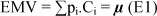
Today a standard quantitative method employed to arrive at an appropriate decision involving risk, in practice, is well-known. The probabilities (pi) associated with possible outcomes (Ci) are multiplied and these products are summed to arrive at a value, referred to as the expected value.3 When expressed in monetary values, it is referred to as the Expected Monetary Value (EMV), with µ being used as the symbol for the EMV; thus:
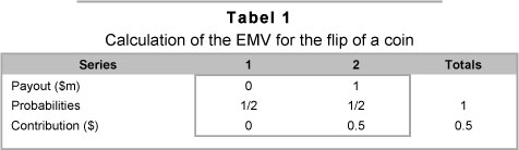
Pierre de Fermat (1601-65) and Blaise Pascal (1623-62) are usually credited with formulating this solution4 dating back to 1654.5 A simple problem can be used to illustrate the calculation. The calculation is independent of the unit of currency used and over the centuries different currencies have been used for the St Petersburg game so for simplicity sake only one unit of currency is used in the article; the dollar. Assume $0m will be paid if on the flip of a coin a tail appears and $1m if a head appears.
The question then is; what is the expected value of this game? There is an equal probability, 1/2 on the flip of a coin, of either a tail or a head appearing, with associated outcomes of $0m and $1m respectively. The ranked sequence of probabilities and outcomes is thus {1/2 , $0m; 1/2 , $1m,}. Using the method described above the EMV is calculated as:

The EMV calculation can also be shown in tabular form as indicated in Table 1, below:
Empirically the game can be played, say, M times and an average of these games obtained. The average of M games with a sum of S is thus:

If an attempt is made to measure the EMV, as an empirical average,  , the empirical value is seldom exactly equal to the expected value as determined by the expected value formula (E1). The reason is simple to understand. If a coin is flipped say 10 times, it is unlikely that there will be exactly 5 heads and 5 tails, and it is even less likely that if a coin is flipped 100 times that there will be exactly 50 heads and 50 tails and so on. There is a wide range of possible outcomes with µ being simply one of those outcomes, albeit the most likely outcome. The range of possible outcomes for
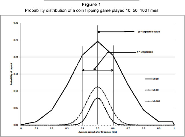
  can be described by a distribution which can be determined from probability theory or simulation. Figure 1 indicates the distribution of possible outcomes when the game is played M times, for three different values of M for an outcome of $1m being paid per game each time a head appears.6
Four observations can be made regarding Figure 1. First there is a family of distributions which are all symmetrical about µ. Second, the apex of the distributions, µ = $0.5m is constant, that is, it is independent of M, the number of games played. Third the probability of achieving a result exactly equal to $0.5m decreases as M increases; ie the probability value at which the apex occurs decreases as M increases. Fourth as M increases the dispersion (λ), about µ, decreases. Thus the empirical value,  ,for any set of games played M times and its relationship to µ, the apex of the distribution, is more accurately described as:
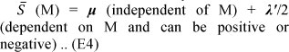
Where λ'/2 is the difference between the empirical average and the expected value, µ,achieved after the game is played M times for any particular series of M games.
The value of dispersion λ in Figure 1, can be pre-selected, say, to include a predetermined area under the distribution curve, say 84 per cent in which case it is anticipated that λ'/2, the empirical result from any series of games played M times, usually will produce a value less than λ/2. As M tends to infinity, the probability of achieving exactly µ tends to zero and λ (M), the dispersion with a pre-selected area under the distribution, also tends to zero. In other words the probability of the EMV equalling µ tends to zero and of being anything but µ also tends to zero. In this case it can be said that the flipping of a coin is subject to both the Central Limit Theorem and the Law of Large Numbers. It is subject to the first because the distribution is symmetrical, about a constant µ, and the second because the dispersion tends to zero as M tends to infinity. And thus when, in practice, the equation EMV = µ is used to solve problems there are unstated and more often than not forgotten assumptions. These are that Central Limit Theorem and Law of Large numbers apply and that a large number of games are involved. These assumptions usually produce a practical outcome approximating µ which is independent of M. These assumptions do not hold for all complex games (Liebovitch & Scheurle, 2000). As is shown below, these assumptions also do not hold for the St Petersburg game.
Having concluded that mathematics, statistics and probability theory can assist the decision maker, the enquiry becomes, what are the questions for which the decision maker requires answers? A casino operator, for example, will want to know if a specific prize is offered for a particular game, say an offer $1m for the coin flipping game, what amount should gamblers be asked to wager to play the game so as to produce an expected profit for the casino? This question is usually posed as what is the fair value of the game? The fair value, in this case is the breakeven value. It is the amount which if paid by gamblers to play games, then the sum of payments received by the casino as income will equal the sum of amounts paid by the casino to gamblers. Thus take as an example the above flipping of the coin game. At $0.5m per game for a 100 games gamblers will pay $50m to the casino and the casino expects to pay back $50m to gamblers. The net expected profit of the casino is thus zero.
There is a second question which can be asked; and that is, what amount is it anticipated that a gambler will be Willing To Pay (WTP), to play a particular game? It can be accepted that when dealing with complex games of chance that gamblers cannot intuitively determine the fair value (break-even value) of the game, but, the fair value can in many cases be calculated by applying probability theory. Generally, as a rule of thumb, it is anticipated that gamblers should be Willing To Pay (WTP) an amount to the same order as the Fair Value, or expected value, of the game. Answering questions about gamblers' Willingness To Pay resides more centrally in fields such as behavioural economics, or consumer behaviour, or psychology, not management science or operations research. How gamblers behave, usually cannot be determined objectively by merely examining the game. The decisions, however, can be observed to arrive at answers. There may well be a sort of weak link between the management science objective fair value and the behavioural economics WTP decisions which is the rule of thumb mentioned above. It is anticipated, from observation, that gamblers should be Willing to Pay amounts in the region predicated by the EMV.
3 The birth of the St Petersburg game - Nicolas Bernoulli 9th September 1713
With this background the origins of the St Petersburg game is examined. The above observations relate to the simple game of flipping a coin but the question then becomes:
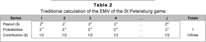
Can the EMV theory developed by Pascal and de Fermat be used with confidence for all games of chance? This was the issue which concerned the Swiss mathematician Nicolas Bernoulli (1687-1759)7. Nicolas devised five games which, in his opinion, clearly demonstrated that gamblers would not make decisions in line with the values determined by the EMV formula. Gamblers' WTP did not in his view coincide with the fair value of the game. It should be noted that his enquiry had shifted from managerial science to behavioural economics. He sent these games in a letter dated the 9th September 1713 to the French mathematician Pierre Rémond de Montmort (1678-1719)8. One of these games, once simplified, is what today is called the St Petersburg game. In this game a coin is flipped until a head appears whereupon the game ceases. The payout starts with $1 and doubles with each flip of the coin. If it appears at the jth flip an amount of $2 j-1 is paid. The traditional EMV for the game can be determined from the method described above giving the result indicated in Table 2.
This gives the traditional solution of:

or
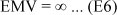
Thus according to the traditional solution the expected value of the St Petersburg game is infinite. However, it is accepted that 'no prudent ... man would be willing to pay even a small number of shillings [dollars]' to play the St Petersburg game (Todhunter, 1865:220). The traditional managerial science solution to the St Petersburg game indicates that the fair value of the game is infinite; suggesting that gamblers should be willing to pay a substantial amount, say $1m per game, but a behavioural economics observation indicates that gamblers are only willing to pay modest amounts. Therein seemingly lies the paradox as explained by Todhunter (1865:220), 'The paradox then is that the mathematical theory is apparently directly opposed to the dictates of common sense.' Theory and behavioural observation thus point in different directions. That is the apparent paradox in decision theory.9
4 "Cardinal" utility solution to the St Petersburg paradox -Daniel Bernoulli 1738
Montmort, exchanged correspondence with Nicolas but in the end did not resolve Nicolas' problems. In a letter dated 22nd March 1715 he indicated that he had already written 16 pages but had not completed the task and doubted if he had the strength to do so. In December 1716 in a letter it is clear he had given up. He died shortly thereafter in 1719. But Nicolas' letter had reached others who suggested solutions to the paradox. The game reached Nicolas' cousin Daniel Bernoulli (1700-82) who included the game in a paper which was published in the 1738 edition of the Papers of the Imperial Academy of the Sciences in Petersburg. Daniel Bernoulli (1738/1954) accepted the traditional solution, EMV = ∞ to be correct and turned his attention from the mathematics of the game to behavioural economics and set about explaining the behaviour of gamblers being only prepared to offer modest amounts. He suggested gamblers do not make a linear evaluation of their possible gains but evaluate possible incremental gains in terms of what he called their "moral expectation." He argued that individuals who add additional incremental wealth to their current fortunes would value the increment as being inversely proportional to their existing wealth. This represents what today is called diminishing marginal utility of wealth. This function he suggested could be described by a natural log function. Thus instead of multi-plying the probabilities and linear gains, he argued that probabilities should be multiplied by the moral expectation of incremental wealth. This approach produces what today is called the expected utility value (EUV) theory.

Using his new theory he worked out how much gamblers would be prepared to gamble as10:

This gives an amount of $2 where Wo = 0; and an amount of $3 where Wo = 10, and an amount of $6 Wo = $1 000 and so on (Todhunter, 1865:220). This modest amount in is line with what was thought gamblers would be willing to pay to play the game. Other solutions, at the time, included one from Cramer who suggested a gambler would be willing to pay $13, again a modest sum.
These low outcomes derived from the moral expectation calculations were consistent with what was thought gamblers would be prepared to offer to play the game. And hence Daniel Bernoulli concluded that a solution to the St Petersburg paradox had been found.11
5 Ordinal utility: Adam Smith (1776), David Ricardo (1817), and Jeremy Bentham (1748-1832) et al.
Daniel Bernoulli's paper appeared to gather dust as a different thread of utility theory moved to centre stage in economics but this thread was derived from another source. Adam Smith in his Wealth of Nations drew attention to the fact that a distinction existed between value in exchange (price) and value in use (usefulness or utility). As illustration he used diamonds that are very expensive. They have a substantial value in exchange, but they are not very useful. On the other hand water is inexpensive but of great value in use. This enigmatic distinction however proved difficult to convert into a comprehensive economic theory despite the efforts of many of the great economists of the time. It was not until the 1870s that three economists, William Stanley Jevons (1835-1882), Leon Walras (1834-1910) and Carl Menger (1840-1921) working separately prompted what is known as the marginal revolution. By the turn of the century it was accepted that utility was difficult to measure and it was impossible to make interpersonal comparisons. A cardinal utility theory appeared to be elusive and it was reluctantly accepted that economics would have to be largely content with ordinal utility12 and preference curves were introduced to assist analysis.
6 Rediscovery of Daniel Bernoulli's cardinal utility - Von Neumann and Morgenstern (1947)
Interest in Bernoulli's "cardinal" expected utility hypothesis was rekindled by the publication of John von Neumann (mathematician) and Oskar Morgenstern's (economist) Theory of Games and Economic Behaviour (1947). They provided a method for individuals to reveal their certainty equivalents13, and by incorporating ordinal utility placed economics on the promised utility foundation which had eluded economists since Adam Smith's diamond-water enigma.14 Bernoulli's original 1738 paper then became a matter of considerable importance but since it was written in Latin it was largely inaccessible to readers. It was translated for the first time into English in 1954. And thus the St Petersburg paradox moved centre stage.
7 Resolving the paradox - correcting the original mathematical error
Strangely in the 300 years which have elapsed since Nicolas Bernoulli set out the game virtually no-one questioned if the traditional derivation of the linear expected monetary value of the game is correct15. That a problem exists with the traditional solution is clear from the following quotation which appears in Daniel Bernoulli's original 1738 paper16:
"The number of cases [M] to be considered here is infinite: in one half (1/2) of the cases [M] the game will end at the first throw, in one quarter (1/22) of the cases [M] it will conclude at the second, in an eighth (1/23) part of the cases [M] with the third, in a sixteenth (1/24) part [M] with the fourth, and so on ... ad infinitum."
That this statement contains an error was noted by Karl Menger (1902-85)17 who was the technical consultant to the 1954 translation of Bernoulli's paper from Latin to English. He noted:
"Since the number of cases is infinite, it is impossible to speak about one half of the cases, one quarter of the cases, etc., and the letter [M] in Bernoulli's argument is meaningless."
Menger did not realise the significance of the error and did not fully correct it. It is a simple matter to correct since M cannot be infinite to derive a solution, M must be allocated a finite value say M=2k. If Bernoulli's method is applied to these games then 2k-1 games end after the first flip, 2k-2 games end after the second flip and so on. If 2k games are played then the following series of games is expected to evolve:

The expected length of the above series is only k in length, not infinite. Since each term in the series contributes 1/2 to the EMV of the above series of games, the above series produces a total of k/2.
To complete the determination of the expected value of M=2k games it must be established if all the games are expected to be within the above series of k terms. It must be checked to see if all the games are accounted for in the series k in length. The above series (E9) is a geometric progression which is easily summed. The sum of series (E9) is 2k - 1. Thus if 2k games are played one game is expected to end outside of the series which is k in length. This one game which progresses beyond the kth term can be any game in the series and can end anywhere after the kth term. If it ends at the kth + 1 term it will contribute 1 to the EMV of the games and there is a 50 per cent probability that it will end at the k+1 term (Vivian 2003).
If it ends anywhere further from the kth + 1 term it will contribute a greater value to the EMV but there is a declining probability that the game will progress further away for the kth term. This additional amount which is contributed to the EMV from the game which ends after the k+1 term can be represented by λ, the value of which depends on where the game in fact ends beyond the k+1 term.
The EMV of playing St Petersburg games once Daniel Bernoulli's error is corrected is thus:

or if expressed in the usual format of µ + λ

Where µ = (k/2 + 1) and is as before the apex of the distribution in this case the distribution of St Petersburg games as indicated in Figure 2. The values of λ with associated probabilities are as follows:

In the St Petersburg game µ = (k/2 + 1) represents the outcome at the apex of the distribution with a confidence level of 50 per cent. In the St Petersburg game µ is not a constant, it is dependent of M the number of games played. This differs from the simple game of flipping a coin discussed above which produces µ, a constant, and thus independent of M. In the St Petersburg game λ on the other hand is independent of M whereas in the game of flipping of a coin λ decreases as M increases. The distribution of the St Petersburg game does not conform to either the Central Limit Theorem or the Law of Large Numbers. Even if the St Petersburg game is played an enormous number of times the expected value is relatively modest. Thus for example if the game is played 264 (18 446 744 073 709 600 000) times the expected value is a mere $33 at a confidence level of 50 per cent. This expected value is nowhere near as large a figure as anticipated by the traditional solution.
If the correct derivation of the EMV is carried out then the expected value of the game becomes finite, modest, and subject to predicable levels of confidence. The modest figure is in line with what it is thought gamblers would be willing to pay to play the game. With the correct derivation, there is no paradox.18 Once the error is realised, corrected and the correct value determined, and it becomes clear that no paradox exists it can be anticipated that the view that the St Petersburg game leads to a paradox will disappear; the myth that the St Petersburg game produces a paradox in decision theory will be dispelled. But entrenched views are resilient and the myth did not disappear. So the question becomes why should the belief in the existence of a paradox cease at this point of time? This article attempts to answer this question. The answer is to be found in a methodological twist to the story of the paradox which is now considered.
8 The methodological twist dispelling the myth of the paradox
The methodological twist involves recalling the influential debate about what is the appropriate methodology to arrive at the truth. This debate started a few decades before the birth of the paradox, was influential at the birth of the paradox and has continued ever since19. Two fundamental methodologies can be identified; the older being Aristotle's Organon (deductive method). This ancient method was disputed and rejected by Sir Francis Bacon in his Novum Organum (observation - inductive method)20. The switch from the one to the other dominated scientific enquiry when Nicolas was writing the letter to Montmort and no doubt played a significant part in the reason for him formulating the problems in the first place. When any new theory is advanced how is the truth of this theory to be established? In terms of Aristotle's Organon truth could be found from reason or logic. Sir Francis rejected this as being sufficient to validate any theory. Validity had to be established empirically; through observation preferably an observation of nature.
Pre-1620: Aristotle's Organon
Before 1620 the dominant methodology was Aristotle's Organon. This can be described as the deductive (syllogistic) or philosophical method of logic. This method rests strongly on belief and thus has a natural affinity with religion. The 1500s and 1600s brought the limitation of this methodology into focus.
For what seemed at the time to be good reasons the almost universally accepted view, was that the sun rotated round the earth, the Ptolemaic system.21 This view also appeared to have Biblical support.22 This belief formed part of the Aristotelian system of an unchanging celestial realm. This view was a product of Organon. However, Nicolaus Copernicus (1473-1543), a Polish astronomer began to form a different view, the heliocentric view, that it was the earth and the other planets which rotated around the sun. He 'sought, with scanty instrumental means, to test by observation the truth it embodied.'23 His views were published contemporaneously with his death as De Revolutionibus orbium coelestrium (libri vi) (1543)24. Copernicus had found a new basis to discover the truth; observation of nature, not deduction. The tide however turned strongly against Copernicus' heliocentric view. In 1615 Roman Inquisition consultants examined the question and pronounced the Copernican theory to be heretical. By this time Galileo (1564-1642), an Italian, and others became convinced that Copernicus' view was correct and with accepting this view that truth could be found from observation, measurement and the application of the mathematical sciences. He published his views in The Assayer (1623). In 1630 he published his Dialogue Concerning the Two Chief World Systems (Ptolemaic and Copernican) in which he inadvertently insulted and ridiculed the Pope. The reaction was swift. He was brought before the Roman Inquisition and sentenced to lifelong house arrest.
Sir Francis Bacon's Novum Organum (1620)
To a perceptive observer it was clear that a new important method of discovering truth had been found, observation, specifically about nature, and then progression via the inductive method. This was the so-called scientific method. The perceptive observer in this case was Sir Francis Bacon, who in England, in 1620 published his views in his Novum Organum. He specifically rejected Aristotle's Organon method. He stated the essence of this new method is in the opening paragraph of the Novum:
'Man, as the ... interpreter of nature ... understands as much as his observations ... permit him and neither knows nor is capable of more'
Knowledge, about nature, comes from making observations of nature which man can understand, explain and interpret. Observation of nature was where the truth was to be found. In doing so man is not to be bound or encumbered by preconceived conclusions arrived at from a purely deductive process. The new scientific age was ushered in as relying merely on Aristotle's Organon deductive system was rejected. This new objective, impersonal observation based system began to dominate all scientific enquiries. Any conclusions which were arrived at had to be validated by observation of nature.
8.1 The natural world of Nicolas and Daniel Bernoulli in 1713 and 1730
Understanding this debate, then, the question becomes what was the natural world observation sought by Nicolas and Daniel Bernoulli in the early 1700s to validate by observation the correctness of the expected monetary value decision theory? A new theory had evolved, the expected monetary value theory, which was to be applied as a solution to making decisions involving risk. To decide if this theory was correct it had to be validated by observation. As pointed out above there are two basic issues involved in games of chance, the study of the game itself (management science) and the study of the behaviour of the gambler, the decision maker, (behavioural economics). In 1713 nothing could be observed about the game itself to validate the correctness of the theory. All that could be observed was the decision of the decision maker. Daniel decided, from observation, that decision makers do not make decisions as predicted by the expected value theory when applied to the St Petersburg game and hence because of this observation the EMV as a general decision theory had to be rejected. That he rejected the EMV as a general theory is clear from the title of his paper and his opening remarks to his paper. His title is "Exposition of a new theory of the measurement of risk" and in paragraph 3 he states emphatically 'The rule [EMV] must be discarded.' He applied the Novum observation methodology to arrive at this conclusion. He argued that from observation of the behaviour of gamblers that it was clear that people do not make decisions in terms of the EMV rule. Therefore since observation trumps hypothesis the EMV rule had to be rejected. The EMV of the St Petersburg game, as determined mathematically at the time was infinite, but the decision maker did not, in fact, make decisions as predicted by the calculation of the EMV of the game. Thus he concluded that the EMV rule had to be discarded. Having created a new solution, his diminishing marginal utility of wealth he triumphantly proclaimed in the Novum observation terminology:
'Since all our propositions harmonize perfectly with experience [Novum] it would be wrong to neglect them as abstractions resting upon precarious hypotheses [Organon]'
Observation had triumphed over hypotheses. Of course his utility solution says nothing about the St Petersburg game itself. It deals exclusively with observations and explanations about decision makers. What decision makers do however is not natural world observation such as observing the actual outcomes when games are played. It is thus the application of the Novum observation methodology, to gamblers and not the game, which produced the utility solution to the St Petersburg game. The methodology produced the paradox. It does not appear as if anyone took a different but equally possible interpretation of the observations of the behaviour of gamblers and that is that gamblers' decisions were pointing to the fact that the mathematical solution to the game was incorrect and if correctly determined it would harmonise with the decisions of gamblers.
Some comments are directed at his approach of observing gamblers and not the game. First in "observing" gamblers Daniel was clearly working in the field of behavioural economics and not that of the management science. This was different to what Pascal and de Fermat were dealing with. They were concerned with management science not behavioural economics. Daniel says nothing about the game itself. In fact a purpose of his paper was to reject the notion that gamblers look only at the game; that is a central thesis of his paper. He concentrated on the observed behaviour of gamblers. Second his observation about gamblers is not an observation of nature but about human behaviour. The Novem methodology was focused primarily on observing nature. It is not clear that observing human behaviour falls within the purview of the Novum methodology at all. Finally although he refers to the modest amounts that gamblers are willing to pay his source on this point is not clear. It does not appear if any experiments were carried out to determine the amounts gamblers are willing to pay to play St Petersburg games until quite recently (Cox, Vjollca & Bodo, 2009; Hayden & Platt, 2009).
8.2 The natural world of 2013
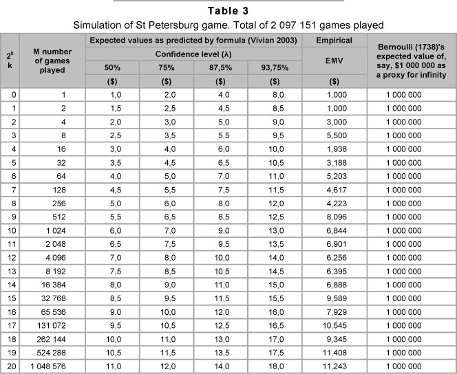
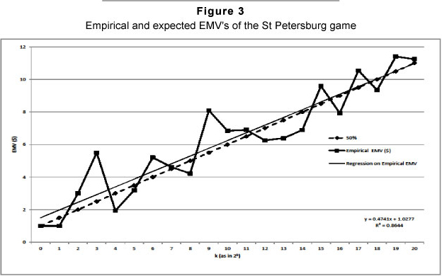
In 2013 things are very different. With the advent of the modern computer outcomes from playing St Petersburg games can easily be observed simply by simulating games. Observations of nature are now available. What happens when games are simulated is indicated below. Table 3 indicates the empirical EMV determined from simulating St Petersburg games when played from 1 game through to 1 048 576 games or a total of 2 097 151 games.25
The results are also shown graphically in Figure 3 with a trend line added. These outcomes are, as noted, observations of nature unlike the observations of gamblers which involve observing human action or behaviour. The following observations can be made about the outcomes recorded in Table 3 and Figure 3.
1) No series of games produced a large empirical EMV. The empirical EMVs ranged from 1 to 11.408. The notion that St Petersburg games produces large average values, say a mere R1 000 000 per game can be discounted as something which simply is not observed in nature.
2) This range of empirical outcomes is in line with amounts which gamblers are thought to be willing to play the game. There is no decision theory paradox.
3) From Figure 3 it is clear that as the number of games increase, the trend produces a line which is upward sloping. Unlike with flipping a coin, the EMV is not constant, ie, it is dependent on M the number of games played. Neither the Central Limit Theorem nor the Law of Large Numbers apply to the St Petersburg game.
4) The results are consistent with the results predicted by the formula EMV = (k/2 + 1) + λ.
5) The observation made by Daniel Bernoulli's (1738/1954) with respect to his utility solution is equally true for the empirical results. The empirical results harmonise with the theoretical results.
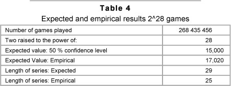
A further simulation was carried out this time with 226 games being played, ie 268 435 456 games. The predicted and empirical results are summarized in Table 4. The expected length of the series is not the traditional infinite series but a series which is expected to contain 29 terms; ie k+1 or 28+1. The empirical length consisted of 25 terms. The expected value is not Bernoulli's infinite value (or a mere $1 000 000 per game, if you like) but a mere $15 (ie k/2+1) at a 50 percent confidence level. The empirical EMV was $17.02. Observation about the game and theoretical predictions harmonise. The detailed results of this simulation are indicated in Table 5.
9 Conclusion
The desktop computer enables any schoolboy nowadays to simulate the St Petersburg game and the game is increasingly being simulated.27 Anyone observing the outcomes of these simulations will notice that the outcomes are never very large as predicted by Bernoulli. It is now simply a matter of time before Bernoulli's solution that the St Petersburg game has an infinite expected value even when a finite number of games are played will be rejected. The view that the St Petersburg game produces a paradox in decision theory likewise will be abandoned, not because it is easy to prove mathematically that that view is incorrect but for the same reason that we no longer believe the earth is flat or the sun rotates around the earth. We can nowadays observe that these things are not true. We can observe that the St Petersburg game does not produce large expected outcomes and hence does not produce a decision theory paradox. Observations from results of nature will dispel the myth of the St Petersburg paradox as observation has dispelled other myths about nature. It is now just a matter of time. If the Bernoullis had the modern computer the paradox would never have seen the light of day. On the other hand, no doubt, the St Petersburg game will be of continued interest for other reasons including the field of behavioural economics.
10 Postscript - prior simulations of St Petersburg games
The thesis of the article is that as the St Petersburg game is being simulated, increasingly, so the traditional view that a paradox exists will be abandoned. It would be incorrect, however, to believe that the St Petersburg game has not been simulated. For the sake of completeness this postscript briefly discusses some of the attempts which have been made to simulate the St Petersburg game. As will be seen the early simulations led to the conclusion that no paradox existed.
Buffon (1777) and earlier simulations
Buffon (1777) appeared to be the first to use simulations to validate probability theory which he applied to the St Petersburg game (Stigler, 1991). Buffon's original work was published in French which has conveniently, for the first time recently, been translated into English and is now generally available (Hey, Neugebauer & Pasca, 2010). Buffon hired a child to flip a coin and recorded the results. The child played 2 048 games. This experiment has been widely discussed (including De Morgan, 1838, De Morgan, 1847, De Morgan, 1915, Moritz, 1923; Stigler, 1991, Aase, 2001). De Morgan (1847) added a further 2 048 games to give a total of 4 096 games (212 games) and the second edition of his work published in 1915 added even more games. Buffon's 2 048 games produced an average of $5 per game. Later an average of $15.4 was determined for the 4 096 games. These combined results were discussed by Moritz (1923). Moritz accepted that if a game is played 2k times it produces what he calls a theoretical value of k/2 and compared this value with the average from the actual playing of the game taken from Buffon's simulation. He reproduces Buffon and De Morgan's (1847) empirical results on a table on page 60 of his article.28 Buffon's simulations, now augmented by that of others produced modest average values which Moritz noted increased as the numbers of games were played (Moritz, 1923:61). Moritz concluded that if 2k games are played this should yield an average of k/2 per game. He then concluded that in fact any pre-selected average for a series of games could be achieved simply by playing the requisite number of games but since it takes time to play the requisite number of games, he noted that insufficient time may exist to achieve the outcome. He noted for example that to secure an average of $18 would require 236 games which he pointed out exceeds the number of seconds in the Christian era. This was of course before the age of the computer. In the face of the results produced by simulation, Moritz concluded that the traditional infinite solution is meaningless (Moritz, 1923: 61). It is suggested that this view is too extreme. More correctly the traditional view is a special case of being correct where an infinite number of games can be played, which is of little practical significance. A more appropriate comment would have been to note that the central limit theorem does not apply and thus that the expected value is dependent on the number of games played.
It is clear that mathematicians at that time had rejected the idea that the St Petersburg game produces a paradox. Feller (1945:302), without reference to Buffon's experiment, specifically dismissed the idea that the St Petersburg game produced a paradox:
'instead of a paradox we reach the conclusion that the price should depend on k, that is to say [the price will] vary as the number of trials increases.'
Feller (1968) repeated this view in his leading textbook.
It should be clear from the propositions set out in this article, that mathematicians in the early to mid-1900s accepted that the average value of games played is a function of the number of games played, is finite and modest and no paradox exists. . These conclusions seemed not to have been noticed, or, were forgotten after the publication of Von Neumann and Morgenstern's (1947) textbook on game theory. These conclusions appear to have remained forgotten ever since despite more recent simulations.
Ceasar (1984) and more recent simulations
More recently Ceasar (1984) simulated St Petersburg games using a computer, producing results for the average values and continued to produce results for Bernoulli's and Cramer's utility solutions. In his simulations the number of games were incremented from 100 to 20 000. He produced a graph for the average value which indicates modest finite outcomes increasing in value as the number of games increase. He demonstrated a wide discrepancy between the mathematical average and the utility solutions. The thrust of his article was to demonstrate that the computer could be used to simulate St Petersburg games and to compare mathematical and utility solutions. The need to resort to manual flipping of the coin was passed. The age of the computer had arrived. The article contains little theoretical discussion.
Russon and Chang (1992)
Russon and Chang (1992) simulate St Petersburg games and find such a wide discrepancy between the simulated average values and traditional predicted value that they suggest a 'practical average' be adopted. Vivian (2004) re-examined their argument and concluded that if the expected value is correctly determined then theory and simulation could be reconciled.
Klyve and Lauren (2011)
The above authors simulate St Petersburg games from 1 000 to 1 000 000 times, producing finite, modest outcomes generally increasing as the number of games increase. They point out that the average per-game winnings depends rather strongly on the number of games played. This, they point out is however, well-known. They attempt to produce a distribution of the St Petersburg game based on Buffon's 2 048 games and end up with a strange distribution which they admit they are at a loss to explain.
Behavioural economics simulations
A large number of simulations has been carried out to test decision makers' Willingness to Pay, many of which involve the St Petersburg game. A discussion of these simulations falls outside the scope of this article but the article by Neugebauer 2010 can be consulted for a detailed discussion on this line of research.
Conclusion re simulations
It is clear that once St Petersburg games are simulated, certain conclusions become inescapable; viz the average values are always finite, modest and increase as increasing numbers of games are played. These observations are at variance with the traditional single value infinite expected value solution to the game. Oddly in the early 1900s once the game was simulated, the idea that the game produced a paradox was rejected, which conclusion seems to have been forgotten. It is this forgotten conclusion that will be rediscovered as the St Petersburg game is increasingly simulated. These simulations, together with the correct derivation of the expected value, spell the end of the myth of the paradox.
Acknowledgement
This article is based on a Senate Lecture delivered on the 15th May 2012. A special word of appreciation is extended to Prof Reekie for comments made on earlier drafts of this article prepared for the Senate Lecture. The usual disclaimers apply
References
AASE, K.K. 2001. On the St Petersburg paradox. Scandinavian Actuarial Journal, 1:69-78. [ Links ]
BACON, F. 1620. The new Organon or the true directions concerning the interpretation of nature. No publisher details. [ Links ]
BERNOULLI, D. 1738/1954. Exposition of a new theory on the measurement of risk. Econometrica, 22(1):23-36. [ Links ]
CLERKE, A.M. 1911. Copernicus - a short biography. Encyclopaedia Britannica. [ Links ]
CEASAR, A.J. 1984. A Monte Carlo simulation related to the St Petersburg Paradox. College Mathematics Journal, 15(4):339-342. [ Links ]
COX, J.C. & VJOLLCA, S. & BODO, V. 2009. On the empirical relevance of the St Petersburg lotteries. Economic Bulletin, 29(1):214-220. [ Links ]
DE MORGAN, A. 1838. An essay on probabilities, Green & Longmans. [ Links ]
DE MORGAN, A. 1847. Formal logic, Taylor & Walton. [ Links ]
DE MORGAN, A. 1915. A budget of paradoxes (2nd ed.) Chicago: Open Court Publishers. [ Links ]
DEVLIN, K. 2008. The unfinished game - Pascal, Fermat and the seventeenth-century letter that made the modern world, Philadelphia, United States; Basic Books. [ Links ]
FELLER, W. 1945. Note on the law of large numbers and 'fair' games. Annals of Mathematical Statistics, 16(3):301-304. [ Links ]
FELLER, W. 1968. An introduction to probability theory and its applications (3rd ed.) New York, USA: John Wiley & Sons Inc. [ Links ]
FRIEDMAN, M. & SAVAGE, L. 1948. The utility analysis of choices involving risk. Journal of Political Economy, 56(4):279-304. [ Links ]
HAYDEN, B.Y. & PLATT, M.L. 2009. The mean, the median and the St Petersburg paradox. Judgment and Decision Making, 4(4). [ Links ]
HEY, J.D., NEUGEBAUER, T.M. & PASCA, C.M. 2010. Georges-Louis Leclerc de Buffon's essays on moral arithmetic. LSF Research Working Paper Series, 10-06. [ Links ]
HIGGS, R. 2011. The dangers of Samuelson's economic method. Independent Review, 15(3):471-476. [ Links ]
JEVONS, W.S. 1897. Elementary lessons in logic: deductive and inductive, London, England: MacMillan and Co. [ Links ]
KLYVE, D. & LAUREN, A. 2011. An empirical approach to the St Petersburg paradox. Mathematical Association of America, 42(4):260-264. [ Links ]
KNÜSEL, L. 1998. On the accuracy of statistical distributions in Microsoft Excel 97. The Statistical Software Newsletter, 375-77. [ Links ]
KNÜSEL, L. 2010. On the accuracy of statistical distributions in Microsoft Excel 2010.' Available at: http://www.csdassn.org/software_reports/Excel2011.pdf [accessed 2012-06-27]. [ Links ]
LIEBOVITCH & SCHEURLE. 2000. Two lessons from fractals and chaos. Complexity, 5:34-43. [ Links ]
MAISTROV, L.E 1974. Probability theory - a historical sketch. New York, USA: Academic Press. [ Links ]
MCCULLOUGH, B.D. & BERRY, W. 2003. On the accuracy of statistical procedures in Microsoft Excel 2007. Computational Statistics and Data Analysis, 49:1244-1252. [ Links ]
MCCULLOUGH, B.D. & HEISER, D.A. 2008. On the accuracy of statistical procedures in Microsoft Excel 2007. Computational Statistics and Data Analysis, 52:4570-4578. [ Links ]
MILL, J.S. 1843. System of Logic 8th 1872. No publisher details. [ Links ]
MORITZ, R.E. 1923. Some curious fallacies in the study of probability. American Mathematical Monthly, 30(2):58-65. [ Links ]
NEUGEBAUER, T. 2010. Moral impossibility in the Petersburg Paradox: a literature survey and experimental evidence. LSF Research Working Paper Series, 10-174. [ Links ]
PETERS, O. 2011. The time resolution of the St Petersburg paradox, Philosophical Transactions of the Royal Society, 369:4913-4931. [ Links ]
RUSSON, M.G. & CHANG, S.J. 1992. Risk aversion and practical expected value: A simulation of the St Petersburg game, Simulation & Gaming, 23:6-19. [ Links ]
SAMUELSON, P.A. 1947. Foundations of economic analysis, Cambridge, Mass: Harvard University Press (there is also a 1965 reprint of the work). [ Links ]
SAMUELSON, P.A. 1952. Economic theory and mathematics - an appraisal. American Economic Review, 42:56-66. [ Links ]
SAMUELSON, P.A. 1977. St Petersburg paradoxes: defanged, dissected, and historically described. Journal of Economic Literature, 15(1):24-55. [ Links ]
STEARNS, S.C. 2000. Daniel Bernoulli (1738): evolution and economics under risk. Journal of Biosciences, 25(3):221-228. [ Links ]
STIGLER, G. 1950. The development of utility theory I & II. Journal of Political Economy, 58(4). [ Links ]
STIGLER, S.M. 1991. Statistical simulation in the nineteenth century, Statistical Science, 6(1):89-97. [ Links ]
TODHUNTER, I. 1865. A history of the mathematical theory of probability - from the time of Pascal to that of Laplace New York, USA; Chelsea Publishing Company 1949. [ Links ]
VIVIAN, R.W. 2003. Solving Daniel Bernoulli's St Petersburg paradox: The paradox which is not and ever was. South African Journal of Economic and Management Sciences, NS 6(2):332-345. [ Links ]
VIVIAN, R.W. 2003a. Considering Samuelson's 'fallacy of the law of large numbers' without utility. South African Journal of Economics, 72(2):363-379. [ Links ]
VIVIAN, R.W. 2004. Simulating Daniel Bernoulli's St Petersburg game: Theoretical and empirical consistency. Simulation & Gaming, 35(4):499-504. [ Links ]
VIVIAN, R.W. 2006. Considering the Pasadena 'Paradox'. SA Journal of Economic and Management Sciences, NS (2):277-284. [ Links ]
VIVIAN, R.W. 2009. Considering the harmonic sequence 'paradox'. SA Journal of Economic and Management Sciences, NS 12(3):385-390. [ Links ]
WHEWELL, W. 1837. History of the inductive sciences. No publisher details. [ Links ]
WHEWELL, W. 1840. The philosophy of the inductive sciences, founded on their history. No publisher details. [ Links ]
VON NEUMANN, J. & OSKAR MORGENSTERN. 1947. The theory of games and economic behaviour. No publisher details. [ Links ]
Accepted: January 2013
Endnotes
1 Risk is used in the sense Frank Knight used it; those situations where the outcomes and their associated probabilities are known.
2 Historically property-casualty insurance products were not priced using probability theory. They were priced using the loss ratio. A relationship between the loss ratio and probability theory can be demonstrated.
3 A word of caution is in order. This method is applicable for games subject to the Central Limit Theorem and Law of Large Numbers. As the St Petersburg game demonstrates, not all games of chance are subject to the Central Limit Theorem and the Law of Large Numbers. The standard method should not be blindly mechanically applied.
4 Samuelson (1977:37) correctly points out that in giving them this credit; they are credited with too much.
5 This history has often been told and increasing detailed histories are appearing. To mention a few; Todhunter (1865), Maistrov (1974); Samuelson (1977), Stearns (2000), Neugebauer (2010), Peters (2011). The paper by Neugebauer in particular is very comprehensive and worth consulting. The famous letters between Pascal to De Fermat were exchanged in1654. A detailed commentary on this correspondence was recently published by Devlin (2008).
6 What happens when M increases, is explained by Vivian (2003a). The distribution for the flipping of a coin is the binomial distribution which is a discrete not continuous distribution, which can approximate the normal distribution. Figure 1 indicates the shape of the distribution as M increases.
7 Nicolas can be spelt in number of ways. The spelling used in this article is taken from the English translation of Daniel Bernoulli's 1738 article.
8 The correspondence is conveniently collected and published by Richard J Pulskamp (1999) at http://www.cs.xu.edu/math/sources/monmort/stpetersburg.pdf.
9 This was described to be the paradox by Todhunter, 1865. It is important to make clear what constitutes the paradox since in more recent articles, authors have claimed to discover further paradoxes but do not indicate, clearly, what they consider to be the paradox; examples of this are the so-called Pasadena and harmonic sequence paradoxes. For a discussion on these recent attempts to create St Petersburg type of paradoxes see Vivian (2006) and Vivian (2009).
10 Todhunter (1865:220), Stigler (1950:374).
11 Bernoulli did not offer any empirical evidence of decisions actually made. In fact empirical evidence had to wait several centuries. Bernoulli (1738:§17) simply concluded, '... our propositions harmonise perfectly with experience...'
12 The history of utility theory was set-out by Stigler (1950)
13 Even before the Theory of Games was available its importance was recognized by leading academics as in the case of Friedman and Savage (1948).
14 In the early 20th century the theory of indifference curves was developed by Edgeworth and others. From this a type of cardinal utility analysis developed. However unlike the von Neumann-Morgenstern 'certainty-equivalent' techniques, that type of cardinal utility (despite the identical terminology) could not provide measurable interpersonal comparisons of utility.
15 The exception may be Feller (1945;1968: 246) discussed below.
16 Daniel Bernoulli (1738/1954 footnote 10).
17 Karl Menger was the son of the Carl Menger mentioned earlier. The original text used N not M. It is changed to M for purposes of the article for the sake of consistency within this article.
18 Vivian (2003) and the simulation verification Vivian (2004).
19 For a recent discussion see Higgs' (2011) discussion of Samuelson's (1952) support of the inductive method and unwarranted disparaging of the deductive method.
20 Bacon's work initiated considerable debate about how knowledge is acquired. See for example Whewell (1837), Whewell (1840), Mill (1843/1872), De Morgan (1847), Jevons (1897). This article does not require any discussion of this debate since the issue of the St Petersburg game is resolved simply by observation. The observation of outcomes of the natural phenomenon which appears when St Petersburg games are simulated are at variance with the predicted traditional theoretical outcome of the St Petersburg game.
21 Galileo in his defence before the Roman Inquisition was able to refer to a surprisingly long list of eminent scientists who held the heliocentric view.
22 Psalm 93:01, Psalm 96:10, Ecclesiastes 1:5 and 1 Chronicles 16:30.
23 Clerke (1911.)
24 Copernicus did not live to see the impact of his work. He was seized with apoplexy and paralysis towards the close of 1542 and died on the 24th May 1543. He also did not live to note the Preface sneaked in by Andreas Osiander insisting that the views in the work were purely of a hypothetical character and not factual.
25 The simulation program was written by Richard J Vivian using Microsoft Excel 2010. It is known that the random Excel generator can be improved (Knüsel 1998, McCullough et al., 2003 and 2008). Knüsel (2010) more recently has opined that the deficiencies identified in earlier versions of Excel are rectified in Excel 2010. Since the purpose of the simulations in this paper are merely to validate the theory, which the simulations achieve, any remaining limitations which may exist in the Excel 2010 random generator are not regarded to be critical.
26 If the Wikipedia entry of the St Petersburg game is examined, a link will be found to an online simulation of the St Petersburg lottery.
27 As pointed out above, theoretically, if the St Petersburg game is played 2k times it produces a series which is expected to be k+1 in length. Moritz's table on page 60 produces a series k in length which Moritz sums to indicate a total of 2k games but if the total is checked it will be noted that one game is missing. He probably could not work out how to account for the missing game, λ in the above theory, and thus simply ignored it.

