


Services on Demand
Article
 English (pdf)
 Article in xml format
 Article references
Indicators

Related links
-
 Cited by Google
 -
 Similars in Google
Share

 Permalink
South African Journal of Economic and Management Sciences
On-line version ISSN 2222-3436
Print version ISSN 1015-8812
S. Afr. j. econ. manag. sci. vol.16 n.1 Pretoria Jan. 2013
ARTICLES
A network branch and bound approach for the traveling salesman model
Elias Munapo
Graduate School of Business and Leadership, University of KwaZulu-Natal
ABSTRACT
This paper presents a network branch and bound approach for solving the traveling salesman problem. The problem is broken into sub-problems, each of which is solved as a minimum spanning tree model. This is easier to solve than either the linear programming-based or assignment models.
Key words: NP hard, traveling salesman problem, spanning tree, branch and bound method
1 Introduction
The traveling salesman problem (TSP) is one of the NP hard problems that are of concern to researchers. A salesman visits each of the given N cities or towns in such a way that each city is visited once, the total distance travelled is minimal and must return to his or her original base (Berman & Karpinski, 2006; Gutin & Punnen, 2006). Up to now we have been unaware of any effective and exact method for solving this problem.
There are several simple variations of the TSP that have originated from various real-life problems. These include the MAX TSP, bottleneck TSP, TSP with multiple visits (TSPM) and clustered TSP. Let G = (V, E) be a graph (directed or undirected) and F be the family of all Hamiltonian cycles (tours) in G. For each edge e ∈ E a cost (weight) Ce is prescribed. The matrix C = (CiJ )NxN is the distance or weight matrix, where the (i, j) th entry cv corresponds to the cost of the edge joining node i to node j in G. Let the node set be V = {1,2,...,N}. In other words, the TSP is to find a tour (Hamiltonian cycle) in G such that the sum of the costs of the edges of the tour is as low as possible.
In the MAX TSP, the objective is to find a tour in G where the total costs of edges of the tour is a maximum. This is solved as a TSP by replacing each edge costs with its additive inverse. In bottleneck TSP, the objective is to find a tour in G such that the highest cost of edges in the tours is as low as possible. A bottleneck TSP can be formulated as a TSP with exponentially high edge costs. In the TSPM we find a routing for travelling salesman who starts at a given node of G, visits each node at least once and comes back to the starting node in such a way that the total distance travelled is minimized. The TSPM is transformed into a TSP by replacing the edge costs with the shortest path distances in G. The node set of G is partitioned into clusters. Then the objective of clustered TSP is to find a least-cost tour in G subject to the constraint that cities within the same cluster must be visited consecutively. This problem can be transformed into a TSP by adding a large cost (LC) to the cost of each inter-cluster edge.
TSP and its variations have a very wide application and span several areas of knowledge which include operations research, computer science, genetics, electronics and logistics. TSP is used in machine sequencing and scheduling. The machine sequencing problem is to find an order in which the jobs are to be processed such that the total machine set up costs are minimized. In some manufacturing systems such as cellular processes, certain products require similar processing and the problem is to group them so as to achieve efficiency and cost reductions. Let G = (V, A ∪ E) be a mixed graph where elements of A are arcs (directed) and elements E are edges (undirected), A1 ⊂ A andE1 ⊂ 5. The arc routing problem is to find a minimum cost closed walk on G containing all arcs in A1 and all edges in E1. The TSP model is also used in creating matrices with certain desired structures which is applied in statistical data analysis and theory of group discussion. Many other applications of TSP models are contained in literature.
2 The TSP model
The objective is to move from node 1 and back in such a way that every node is visited once and the total distance is minimized. It is also assumed that two arcs emanate from each of the nodes.
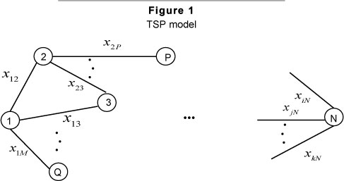
The objective is to move from node 1 and back in such a way that every node is visited exactly once and the total distance minimized. It is also assumed that each node has at least two arcs.
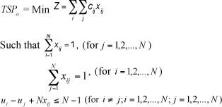
All uj > 0 and xij is a binary variable.
Where Cij is the distance from city i to city j for i ≠ j.
Letting Cii = M, where M is very large relative to the actual distances between the cities ensures that the movement to city i immediately after leaving city i is not possible.
3 Solving the TSP
There are two main categories of TSP which are symmetric and asymmetric. If the distance between two nodes in the TSP network is the same in both directions, then the TSP is called symmetric, otherwise it is referred to as asymmetric. We are not aware of any efficient exact method for solving the traveling salesman problem. There are several heuristics (see Berman & Kapinski, 2006; Gutin & Punnen , 2006; Wolsey, 1980; Winston, 2004) and for exact approaches (see Gutin & Punnen, 2006; Nadef, 2002; Padberg & Rinald 1991; Winston, 2004) available in the literature.
3. 1 Heuristics
These are approximation methods that quickly l e ad to good solutions which are not necessarily optimal. There are several classes of heuristics, some of which are:
- constructive heuristics;
- iterative improvement;
- randomized improvement.
More information on each class of these heuristic s can be found in writing by Berman & Kapinski (2006), Gutin & Punnen (2006) or Wolsey (1980). Even though some of these approximating methods have improved we cannot be sure how far these approximated solutions are from the optimal ones. For example when all the towns in very large countries such as Russia, USA or China are visited, the difference between the exact and approximate solutions may amount to millions of dollars.
3.2 Exact approaches
The most obvious exact approach is to try all the possible routes to decide which one is the best. The worst cost for this approach is of factor O(n!) and is not practical for a large number of towns. Other exact approaches include
- Linear programming (LP) based branch and cut methods (see Gutin & Punnen, 2006; Karlof, 2005; Mitchell, 2001; Nemhauser & Wolsey, 1988);
- Branch and bound methods with assignment sub-problems (see Winston, 2004);
- Dynamic programming techniques (see Gutin & Punnen, 2006).
Efforts to improve these exact approaches have been unsuccessful. Large amounts of computational times are required. The computational times for these exact approaches are not practical since decisions have to be made urgently in war or disaster situations.
4 Network branch and bound approach
In this paper an exact branch and bound approach is proposed. The network branch and bound uses minimum spanning trees (MST) as sub-problems. The minimum spanning tree can be solved efficiently by the available approaches. The MST model is easier to solve than either the LP-based or assignment sub-problems that are currently used. In this paper the following definitions apply.
4.1 Definitions
A tree is a set of nodes that are connected by arcs to form a single structure.
A leaf is a node that has no children and is connected to a tree.

Node 1 is an example of a leaf. Clearly it has no children.
For a network with N nodes, a spanning tree is a group of n -1 arcs connecting all nodes of the network and contains no loops.
Minimum spanning tree (MST)
A spanning tree of minimum length in a network is called a minimum spanning tree.
4.2 MST algorithm
The minimum spanning tree algorithm is used to find the minimum spanning tree for a given network. The algorithm comprises of the following steps.
Step One: Begin at any node i and join node i to node j, closest to node i. The two nodes i and j now form a connected set of nodes C = {i, j} and arc (i, j) will be in the minimum spanning tree. The remaining nodes in the network ( ) are the unconnected set of nodes.
Step Two: Choose a member of (n) that is closest to some node in C. Let m represent the node in C that is closest to n. Then the arc (m,n) will be the minimum spanning tree. Update C and . Since n is now connected to {i, j}, C now equals {i, j,n}, and we must eliminate node n from .
Step Three: Repeat this process until a minimum spanning tree is found. Ties for the closest node and arc are broken arbitrarily. In this paper preference is given to the arc that is least likely to form a leaf. The strategy of the algorithm proposed in this paper lies in solving the TSP as an MST and then using branching to remove leaves.
Theorem 1
The MST algorithm finds a minimum spanning tree.
4.2.1 Proof by contradiction:
Let
S be the minimum spanning tree,
Ck be the nodes connected after iteration k of MST has been completed,
be the nodes not connected after iteration k of MST has been completed,
Ak be the set of arcs in the minimum spanning tree after k iterations of MST algorithm have been completed.
Suppose that the MST algorithm does not yield a minimum spanning tree.
Then the arc chosen at iteration k (ak) is not in S, i.e., ak ∉ S.
All arcs in Ak-1 are in S, i.e., Ak_x ⊂ S. This implies ak ∈. S and ak leads from node in Ck-1 _jto a node Ck-1.
Replacing ak with ak, we obtain a spanning tree shorter than S.
The contradiction proves that all arcs chosen by the MST must be in S. The MST algorithm does indeed find a minimum spanning tree. This proof can be found in books such as Gutin and Punnen (2006).
4.3 TSP tree, transformation and arc fixing
TSP tree
Is an MST without leaves other than the first and last nodes.
Transforming a spanning tree
Branching can be used to transform any MST into TSP.
Fixing an arc
The MST algorithm uses n -1 arcs to connect the nodes in the network, but the optimal solution of the TSP must have n arcs. This problem can be alleviated if one arc which is part of the optimal tour is known before the problem is solved. Unfortunately this arc is not known. In the optimal tour exactly two arcs are used in completing a tour at every node. With this knowledge arcs can be fixed and the necessary branching done so as to remove the unwanted leaves from a current minimal spanning tree. Let the number of arcs at a node i be l.
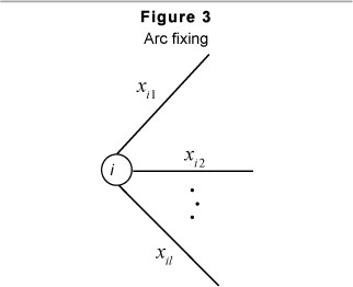
Arc fixing way 1: If a single arc is fixed then
Xil + χ i2 + ... + Xil = 1.
There will be a total of l sub-problems (SB) as shown in Figure 4 below.

The sub-problems SB1,SB2,...,SBl are mutually exclusive subsets of TSP.
SB, ∪ SB2 ∪...∪SB, = TSP
For α ≠ β
SBa∩ SBβ = ∅
Fixed value in the hth branch is given by Fh and is the value of a single arc. Fixing way 1 is done before applying the spanning tree procedure. The fixed arc is removed from the TSP before applying the spanning tree procedure.
Arc fixing way 2: At every node exactly two arcs are used in completing the tour. This is because at any node we must have one arc in and one arc out for us to complete the tour. This is also referred to as the one arc in and one arc out rule.
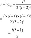
Fixing of two arcs at node i will result in  sub-problems (SP) or branches.
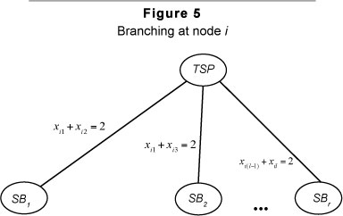
Where  The number of sub-problems (r) formed by branching is given by
Also the sub-problems SB1,SB2,...,SBr are mutually exclusive subsets of TSP.
SB1 ⊂ SB2 ⊂...⊂SBr = TSP
For α ≠ β
SBa ∩ SBp =∅
Fixed value in the hth branch is given by Fh and is the sum of two arcs.
Fixing way two is also done before applying the spanning tree procedure. The two fixed arcs and an included node i are removed from the TSP before applying the spanning tree procedure.
Theorem 2
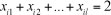
Any sub-problem that results in at least one leaf in the network structure is infeasible. From the definition of a TSP at node i,
xa + xi2 +... + xil = 2.
This is referred to as the one arc in and one arc out rule.
Proof: A leaf occurs when
xil + xi2 +...+ xil = 1.
This is infeasible to the one arc in and one arc out rule. Two arcs are required to pass through a node.
4.4 Removing leaves in an MST
Besides fixing arcs, branching is also used to remove leaves in MST. A branch fathoms • if the sub-problem becomes infeasible;
- if the MST for the sub-problem is also a TSP; and
- or if the objective value given by the sub-problem is larger than some given lower bound (LB).
4.4.1 Theorem 3
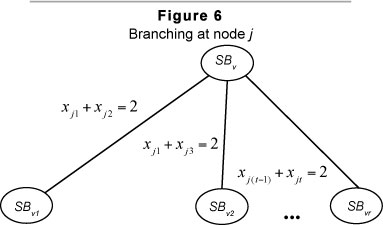
Any node j is selected for branching
a) if the number of arcs is greater than two, i.e., xjl + xj2 + - + xjt > 2.
b) if it has the smallest number of arcs emanating from it.
Where t is the number of arcs emanating from node j.
Proof (a)
Branching is done to enforce the restriction, Xjl + Xj2 + - + Xjt = 2.
This can be done if the number of arcs is two or more, i.e. xfl + xj2 + ... + xjt > 2.
Where
- SBv is the sub-problem after the vth iteration;
- SBvk is the kth branch at kth node. Similarly the number of sub-problems (vr) formed by branching is given by

The sub-problems SBv1,SBv2,...,SBvr are also mutually exclusive subsets of SBv.
SBvl ∪ SBv2 ∪... ∪ SBvr = SBv
For δ ≠ λ
SBa Π SBÍ = 0
Proof (b)
Let the number of arcs emanating from node i be given by t.. The number of arcs at this node is directly proportional to the number of sub-problems ri generated by branching at node i. i.e.
ti ~ ri
Suppose we are selecting nodes in an in increasing order of the number of arcs i.e.
r1 < r2 <...< rN
Where N is the number of nodes in the TSP and node 1 has the least number of arcs followed by node 2, then node 3 in that order up to variable node N. When the algorithm is applied the following sub-problems are visited in the search process. The worst case is assumed in the search process.
Starting with the most restricted variable
Stage 1: number of sub-problems visited = r1
Stage 2: number of sub-problems visited = r1r2;
Stage N: number of sub-problems visited = r1r2...rN
The total number of sub-problems (τ A) is:

Starting with the least restricted variable
Stage 1: number of sub-problems visited = rN; Stage 2: number of sub-problems visited =rNrN-1;
Stage N: number of sub-problems visited =rNrN-1...r1 Total number of nodes (τΒ) is:
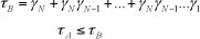
It is computationally cheaper to start with node with the least number of arcs.
4.5 The TSP - MST inequality
The objective value (SUB(MSTo)) of any sub-problem obtained by solving as MST plus a fixed value (Fv) from one of the arcs is less than or equal to the optimal tour (SUB(TSPo) of the sub-problem.
SUB(MSTo ) + Fv < SUB(TSPo )
Proof
SUB(MST0) + Fv -Fv < SUB(TSPC) -Fv
SUB(MSTo) < SUB(TSPo) - Fv
Let SUB(TSPo) - Fv = Ts,where a Ts is a spanning tree structure.
Then
SUB(MSTo) < Ts
If
SUB(MSTo) = Ts
Then Ts is a tree structure without any leaves but connects all the nodes.
This is valid, as SUB(MST) is the smallest sum of (n -1) arcs used to connect all the nodes in any network structure where loops are not acceptable. Loops are not possible in Ts as one arc has been fixed.
4.6 Network branch and bound approach
Steps of the network branch and bound algorithm are summarized as follows.
Step 1: Select the node with the least number of arcs (l). Fix these arcs by branching into l sub-problems (way 1) or  sub-problems (way 2).
Step 2: Solve each sub-problem generated in Step 1 as MST. A sub-problem fathoms
- if it becomes infeasible;
- if the MST for the sub-problem is also a TSP; and
- or if the objective value given by the sub-problem is larger than some given lower bound (LB) obtained in an earlier sub-problem. The optimal tour is given as the sub-problem with the overall shortest tour.
Else go to Step 3.
Step 3: From those MST with leaves select the node associated with the least number of arcs. (t). Branch into  sub-problems and return to Step 2.
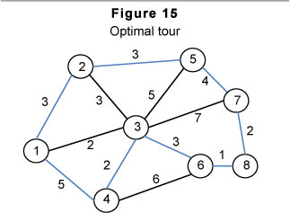
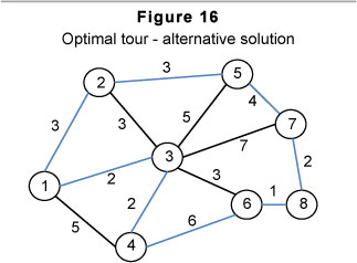
4.7 Optimality
The solution obtained when using the network branch and bound is exact.
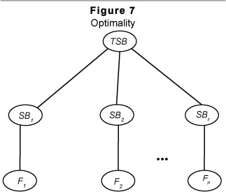
Where Fj is the fathomed sub-problem and µ is the number of fathomed sub-problems, TSPo = min [F1, F2,...,Fµ]= SUB(MSTo).
4.8 Numerical illustration
Use the network branch and bound to solve the following TSP.
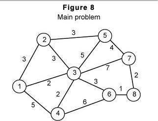
4.8.1 Solution using the network branch and bound method
The node with the least number of arcs is node 8. Fixing can be done in two ways. Way 1 is to fix either arc 6-8 or arc 7-8. This is done by using x68 + x78 = 1 to branch into two sub-problems. Way 2 is done by using x68 + x78 = 2 to branch into a single sub-problem  .
.
The two ways will produce the same solution and way 2 is arbitrarily selected for this illustration. Fixing is done by removing the two arcs 6-8 and 7-8 and the included node 8 from the TSP network diagram. The network diagram reduces to 7 nodes and 12 arcs, as shown below in Figure 9.
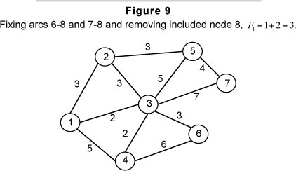
Applying the minimum spanning tree algorithm, we have Figure 10.
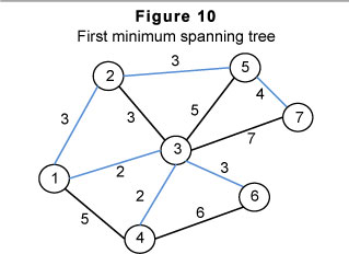
Selecting node 4 as the only leaf we have,

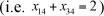
The equation implies the number of subproblems is given by

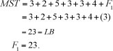
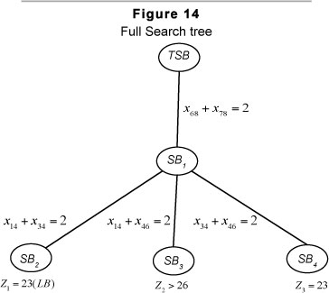
Sub-problem 2
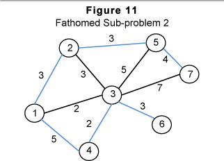
Sub-problem 3
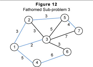
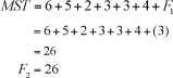
This sub-problem has fathomed, since 2 F is greater than the lower bound (LB) given earlier in sub-problem 2.
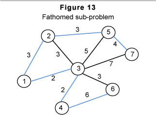
Sub-problem 4

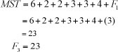
The sub-problem has fathomed, since the minimum spanning tree does not have leaves. The network branch and bound algorithm full search tree is presented in Fig 13.

7 Conclusion
The algorithm proposed in this paper uses spanning tree approaches as sub-problems in solving the difficult traveling salesman problem. A spanning tree approach is more efficient than either the LP based or the assignment sub-problems. For small TSP models it makes sense to use way 2 for fixing arcs since the number of branches is given by  . This number of branches increases rapidly with an increase in the number of arcs. Thus for large TSP models it is wise to use way 1 since the number of branches is just l. The strength of the approach lies in the fact that the number of arcs on the various nodes of practical problems is not the same. Our strategy is to target those nodes that have the smallest number of arcs to form branches. At the moment large amounts of money are being wasted the world over by sales persons, rubbish trucks, delivery or postal companies and other organizations because exact solutions for routing problems cannot be determined and used in acceptable times. The network branch and bound approach proposed in this paper is still in its early stages of development and more effort will be put into refining it so that it reaches its full computational efficiency level. In future efficiency tests for this algorithm will be conducted on standard benchmark TSP instances.
References
BERMAN, P. & KARPINSKI, M. 2006. 8/7-Approximation algorithm for (1,2)-TSP. Proc. 17th ACM-SIAM SODA conference:641-648. [ Links ]
GUTIN, G. & PUNNEN, A.P. 2006. The traveling sa/esman problem and its variants. Heidelberg: Springer. [ Links ] KARLOF, J.K. 2005. Integer programming: theory and practice. Boca Raton FL: CRC Press Inc. [ Links ]
MITCHELL, J.E. 2001. Branch and cut algorithms for integer programming: In Floudas, C.A. & Pardalos, P.M. (eds.) Encyclopedia of optimization. Boston: Kluwer Academic Publishers. [ Links ]
NADEF, D. 2002. Polyhedral theory and branch and cut algorithms for the symmetric TSP. In: Gutin, G. & Punnen, A. (eds.) The traveling salesman problem and its variations. Dordrecht: Kluwer:29-116. [ Links ]
NEMHAUSER, G.L. & WOLSEY, L.A. 1988. Integer and combinatorial optimization. New York: John Wiley. [ Links ]
PADBERG, M. & RINALDI, G. 1991. A branch and cut algorithm for the resolution of large-scale symmetric traveling salesman problems. SIAM Review, 33(1):60-100. [ Links ]
WINSTON, W.L. 2004. Operations research applications and algorithms (4th ed.) Boston: Duxbury Press. [ Links ]
WOLSEY, L. A. 1980. Heuristics analysis, linear programming and branch and Bound. Mathematical Programming Study, 13:121-134. [ Links ]
Accepted: June 2012

