


Services on Demand
Article
 English (pdf)
 Article in xml format
 Article references
Indicators

Related links
-
 Cited by Google
 -
 Similars in Google
Share

 Permalink
South African Journal of Economic and Management Sciences
On-line version ISSN 2222-3436
Print version ISSN 1015-8812
S. Afr. j. econ. manag. sci. vol.15 n.2 Pretoria Jan. 2012
ARTICLES
Fiscal regime changes and the sustainability of fiscal imbalance in South Africa: a smooth transition error-correction approach
Samuel S Jibao; Niek J Schoeman; Ruthira Naraidoo
Department of Economics, University of Pretoria
ABSTRACT
In addition to the conventional linear cointegration test, this paper tests the asymmetry relationship between fiscal revenue and expenditure, by making a distinction between the adjustment of positive (budget surplus) and negative (budget deficit) deviations from equilibrium. The analysis uses quarterly data for South Africa. The paper reveals that government authorities in South Africa are more likely to react more quickly when the budget is in deficit than when in surplus, and that the stabilisation measures used by government are fairly neutral at low deficit levels; that is, at deficit levels of 4 per cent of GDP and below. We conclude that the assumption that adjustment towards equilibrium is always present and of the same strength under all circumstances, is not valid in the case of fiscal data on South Africa; and that that fiscal sustainability in South Africa has been attained at the expense of a reduction in the ratio of expenditure to GDP on education, and a relatively constant ratio of expenditure to GDP on health. The paper noted that a priori one would expect that such a decline in the allocations to sectors which could stimulate growth and which in turn could generate future revenue, may pose a threat to the accumulated fiscal space. In South Africa the main fiscal challenge, therefore, is to find ways through which the recent gains in fiscal solvency can be consolidated.
Key words: smooth transition error correction model; nonlinearity; government inter-temporal budget constraint; and fiscal sustainability
JEL: C22, 51, H62
1 Introduction
Developments which followed the sub-prime crisis have led to renewed debate on fiscal sustainability: the massive degree of fiscal intervention, with corresponding increases in deficits and debt, are a concern. From a fiscal perspective, maintaining a stable long-term relation between expenditures and revenues is one of the key requirements for a stable macroeconomic environment and a sustainable economy. Sustainability, in general, concerns current and expected policies. If economic agents do not expect current and future policies to operate within the inter-temporal budget constraint, then the fiscal process would be unsustainable and government insolvency possible.
Several of the empirical studies on fiscal sustainability, however, focus on the time series behaviour of tax revenues and expenditures, as well as debt series, to investigate whether the behaviour of these series is consistent with the inter-temporal budget balance. The empirical results of these studies vary depending on the sample period and the methodology used. In the United States, Cunado, Gil-Alana, and Perez de Gracia (2004), Hamilton and Flavin (1986), and Trehan and Walsh (1988) failed to reject the inter-temporal budget balance, whilst Hakkio and Rush (1991), Wilcox (1989) and others rejected it. Empirical investigations into government's inter-temporal fiscal solvency constraints in East Asia have also been documented (see for example, Baharumshah & Lau 2007). Based on time series analysis and quarterly data over three decades, Baharumshah and Lau (2007) found evidence of sustainable fiscal finances in Thailand and South Korea, whilst the Philippines and Malaysia demonstrated only 'weak sustainability'. Baharumshah and Lau (2007) showed that in Singapore, revenue was growing at a faster rate than government spending.
In South Africa, issues of fiscal sustainability received greater attention in the 1980s and 1990s following a growing public debt/GDP ratio. In the early 1980s, the South African economy became a closed economy following the economic sanctions by the international community. As a way of alleviating the effect of the sanctions, the said economy became highly subsidised by the government. The government introduced the industrial decentralisation programme which amounted to direct and indirect subsidies for the establishment of large industrial companies. In addition, because the government was involved in proxy wars in and around South Africa, government expenditure increased significantly during the same period (Caner & Schoeman, 2006). Increased government expenditures and debt service forced the government to increase taxation to finance future expenditure. The period beginning in the early 1980s and ending with the transition to a new constitutional and political environment was therefore marked by increasing government expenditures and taxation, with fiscal deficit increasing to 6.8 per cent in 1993.
In the earlier and mid-1990s, therefore, several researchers argued that fiscal policy was unsustainable in South Africa (Roux, 1993; Van der Merwe, 1994; Schoeman, 1994; Cronje, 1995). Roux (1993) argued that the South African government would be able to finance higher social expenditure only if economic growth improved; otherwise, debt-financed increases in social expenditure would cause an increase in the public debt/GDP ratio. Van der Merwe (1994) argued that fiscal policy in South Africa is unsustainable due to the large gap between real interest rates and real economic growth as well as the relatively large size of the deficit. Schoeman (1994) also warned that as long as government runs a large deficit in the face of a real interest rate that exceeds the real economic growth, the public debt/GDP ratio would tend to explode.
Consistent with the findings of the various researchers in South Africa, the South African economy has embarked on broadly three phases of fiscal reform since 1994.
From 1994 to 1996, following a period of recession and a rapid rise in the budget deficit, Government's Reconstruction and Development Programme was phased into departmental plans and budgets, and a comprehensive reprioritization of public expenditure was undertaken (Manuel, 2004). The average budget deficit stood at 4.3 per cent of GDP and government debt was approaching 50 per cent of GDP by 1994.
A period of fiscal consolidation from 1997 to 2000 saw the introduction of medium term expenditure planning, substantial investment in tax reform and revenue administration capacity, and efficient coordination of fiscal and monetary policy. The budget deficit declined to 3.0 per cent of GDP, public debt relative to GDP declined from 49.7 per cent in 1994 to 44.4 per cent in 2000 and average borrowing costs decreased sharply, providing room for government to spend more on social services and infrastructure.
From 2001 to 2008, the government of South Africa adopted a more prudent fiscal stance. The fiscal deficit as a percentage of GDP declined from an average of 4.6 per cent from 1992 to 19991 to an average of 1.3 per cent from 2001 to 2005, and thereafter recorded a budget surplus in 2006 and 2007 of 0.3 per cent and 0.7 per cent of GDP respectively2.
Although government had achieved a substantial reduction in its budget deficit target, from 6.8 per cent of GDP in 1993 to 0.6 per cent in 2008, the scenario has meanwhile changed again (see Budget Review, 2010), mainly due to the slowdown in the world economy, which also affected the revenue base of the South African economy. However, the policy of fiscal prudence during the period 2003 to 2008 resulted in a substantial decline in real debt service cost, while the real growth rate of the economy increased considerably. Nevertheless, there still exist a gap between the real debt service cost and the real growth rate since the former exceeds the latter.3 Furthermore, it appears that public debt and budget deficit reductions have been achieved at the expense of a relative reduction in service delivery expenditure, as is evident in the reduction in the ratio of education expenditure to GDP from an average of 6.21 per cent during the period 1990 to 1999, to an average of 5.6 per cent during the period 2000 to 2008; and a reduction in health expenditure relative to GDP to an average of 2.84 percent between 2000 to 2008 from 1990 to 1999 average of 2.93 per cent.4
In most of the studies recorded in the literature on fiscal measures to address the solvency condition, researchers have either tested for linear stationarity in the total government deficit series or tested for linear cointegration between total government spending and total tax revenues. To the best of our understanding, few researchers have used non-linear techniques to quantify the adjustment process of fiscal and other macroeconomic variables towards the long-run equilibrium (Van Dijk & Franses, 1997; Hansen & Kim, 1996; Kunst, 1992 & 1995; Dwyer, 1996; Swanson, 1996; Cipollini, 2001). In South Africa in particular, no study has tested whether the error-correction process used in the respective studies is linear. Instead, previous studies have assumed that the adjustment process driving the variables toward equilibrium is linear; i.e. adjustment towards equilibrium is always present and of the same strength under all circumstances. In this study the authors want to point out that there are situations in which the validity of this assumption might be questioned (Van Dijk & Franses, 1997).
The authors therefore apply an extension of the linear inter-temporal budget constraint rule of fiscal sustainability to a regime-switching framework, where the transition from one regime to the other occurs in a smooth way. The switching between regimes is controlled by the state of the fiscal balance. This feature of the smooth transition model allows us to test the ability of high against low budget deficits or surpluses to best describe the non-linear dynamics of fiscal policy in South Africa.
Following the introduction, Section II presents sustainability criteria as obtained from the literature. Section III provides the estimation procedures, with both linear and non-linear specifications; Section VI presents the results from the estimations and the last section summarises and concludes.
2 Sustainability criteria
The most straightforward way to assess the fiscal sustainability position is to start from a government's inter-temporal budget constraint. The budget constraint looks at the long-run relationship between government revenue and expenditure (that covers the total government spending on goods and services, transfer payments and interest on debts). For simplicity, assume that budget deficits are financed using bonds with a maturity of one period. This implies that the government faces the budget constraint as shown in equation one:

where G is government expenditure, r is the one-period real rate of interest, R is government revenue and B is the stock of debt. Iterating equation (1) forward yields the government's inter-temporal budget constraint:

We assume that the real interest rate is stationary with unconditional mean given by r and also that the growth rate of the real supply of bonds, on average, is equal to or lower than the average rate of interest (Hamilton & Flavin, 1986; Haug, 1995). With these assumptions, we can have the following expression:

The above equation (3) states that the debt stock, when measured in present value terms, vanishes in the limit. By definition, it excludes Ponzi financing; that is, the government is not 'bubble'-financing its expenditure by issuing new debt to finance the deficit. This is equivalent to saying that the deficit is sustainable if and only if the stock of debt held by the public is expected to grow no faster than the mean real rate of interest, which is viewed as a proxy for the growth rate of the economy (Baharumshah & Lau, 2007).
Following equation (3), the inter-temporal budget constraint, equation (2), can be rewritten as:

The inter-temporal budget constraint, under the no-Ponzi scheme rule, imposes restrictions on the time series properties of government expenditure and revenue given by the right hand side of equation 4. This will be stationary, as long as government expenditure, revenue and the stock of debt are all stationary in first differences. Specifically, if Gt are Rt I(1), they will be cointegrated, implying that there exists an error-correction mechanism pushing government finances towards the levels required by the inter-temporal budget constraint (Baharumshah & Lau, 2007).
Assuming that the transversality condition for the budget constraint holds and the limit term in equation (3) is zero, we arrive at the following cointegrating relationship as shown in equation 5 (Hakkio & Rush, 1991);

Where 'dlev't and 'dlexp't are the differenced revenue- to- GDP and expenditure-to- GDP variables in the current period. A priori, we expect a positive and significant relationship between government expenditure-to-GDP and its revenue-to-GDP. To choose the lag lengths, we follow the suggestions of Terasvirta (1994) by considering a number of test statistics on the error correction model (VECM) specifications; and Cipollini (2001) by using the likelihood ratio sequential tests on the residuals. Using the information criteria, the Schwarz Information Criterion and the Hannan-Quinn Information Criterion (HQ) suggest lag length of 3, whilst the Akaike Information Criterion (AIC) and the Final Prediction Error (FPE) suggest lag length 5. However, like Cipollini (2001) we chose lag 8 as the optimal lag length since this lag order gives evidence of homoscedastic and serially independent residuals.
3 Specification and estimation techniques
In this paper, our empirical estimation involves the following steps: (i) testing for stationarity of the variables; (ii) testing for cointegration and estimation of the cointegrating relation; (iii) testing for non-linearity of the adjustment process; and (iv) estimating and evaluating of the smooth transition error correction model.
3.1 Linear estimation techniques
We carry out three different tests for the order of integration which are: the Augmented Dickey-Fuller (1981), the Kwiatkowski, Phillips, Schmidt and Shin (1992) and the Phillips-
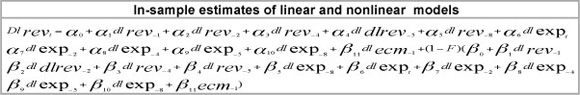
Following Martin (2000), the deficit is 'strongly' sustainable (strong solvency) if and only if the I(1) process of R and G are cointegrated and β =1. The deficit is only 'weakly' sustainable if R and G are cointegrated and 0<b<1 (see Trehan & Walsh, 1988; Quintos, 1995). The linear model estimated in this paper, after eliminating insignificant lags, is specified as:

Perron (1988) tests. The Dickey-Fuller and Phillips-Perron tests have as their null hypothesis that the dynamics of the respective series are characterised by a unit root. The Kwiatkowski, Phillips, Schmidt and Shin test, on the other hand, is based on the null of stationarity. The use of three tests is justified since Phillips and Perron (1988) and Zivot and Andrews (1992) have demonstrated that the Augmented Dickey-Fuller test has low power in the presence of a structural break.
We consider those cointegration tests that are most popular among researchers: the residual-based test suggested by Engle and Granger (1987) and the Likelihood Ratio test introduced by Johansen (1991). Given a bivariate case (for simplicity) with no deterministic regressors, the residual-based test for cointegration is performed via the two-step procedure of Engle and Granger (1987). That is, we first estimate the cointegration regression as specified in equation (7) using ordinary least square (OLS) and second, test for the presence of a unit root in the regression residuals.

Johansen (1991) advocates a test for cointegration by testing the rank r of p by applying likelihood ratio tests to test the significance of the squared partial canonical correlations between  and yt-1 denoted
  and
and  which can be obtained by solving a generalised eigenvalue problem. The authors use trace tests to test H0:r = r0 against the alternative hypothesis H1:>- r0+1 for r0 = 0,1.
This paper considers both non-parametric and parametric tests for linearity. The non- parametric test follows Brock-Dechert-Scheinkman (1987). It tests the null hypothesis of independence and identically distributed variables against an unspecified alternative. The Brock-Dechert-Scheinkman (1987) test cannot test chaos directly, but only non-linearity, provided that any linear dependence has been removed from the data (e.g. using traditional ARIMA-type models or using first differences). The Brock-Dechert-Scheinkman (1987) statistics are, therefore, different from other non-parametric test statistics since these focuses mainly on either the second- or third-order properties of x2. The basic idea of the Brock-Dechert-Scheinkman (1987) test is to make use of a 'correlation integral' popular in chaotic time series analysis. Given a kdimensional time series and observations  , define the correlation integral as:5

where Id (u,V)is an indicator variable that equals one if  , and zero otherwise, and where
  is sup norm. The null hypothesis of the BDS test is that the series is linear and the alternative hypothesis is that the time series is non-linear after removing any linear dependence from the data, either by using ARIMA-type models or taking the first difference of the series. This test statistic has a standard normal limiting distribution.
The parametric test for linearity follows Teräsvirta (1994) who suggests a method of approximating the transition function by a Taylor expansion about the null of linearity g = 0. The linearity test involves estimating an auxiliary regression by OLS:
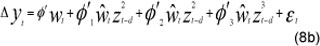
where
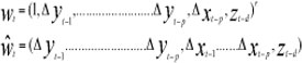
The original null hypothesis of linearity, H0: y = 0 is equivalent to the hypothesis that all coefficients of the auxiliary regressors  are zero i.e.H'0:f1=f2=f3=0. For details on the LM-type test for this hypothesis, see Van Dijk et al. (1997). To select the most appropriate lag of zt to use as transition variable, the test should be carried out for a number of different values of d, say d = 1 ...D. If the linearity is rejected for several values of d, the one with the smallest p-value is selected as the transition variable; see Van Dijk et al. (1997).
3.2 Non-linear estimation technique
If the linearity hypothesis is rejected, we can estimate a non-linear model using non-linear least squares (NLS). In this paper, we apply the smooth-transition threshold models (Granger & Teräsvirta, 1993; Teräsvirta, 1994; Teräsvirta, (1998) which allow for smooth transition between regimes of behaviour and thus generalise the threshold autoregressive model (TAR). The other strength of the smooth transition model is that it is theoretically more appealing than the simple TAR models that impose an abrupt switch in parameter values. An abrupt switch only happens if all agents act simultaneously. Additionally, the STR model allows different types of market behaviour depending on the nature of the transition function. In particular, the logistics function allows differing behaviour depending on whether deviations from equilibrium are positive or negative, whilst the exponential function allows differing behaviour to occur for large and small deviations regardless of sign (see McMillan, 2004). Following McMillan, the STR model is given by equation 9 below:
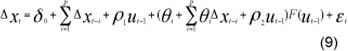
where F(ut-d) is the transition function and ut-d the transition variable. The logistic function is given as follows, with the full model thus referred to as a logistic STR (or LSTR) model:
![]()
which allows a smooth transition between the differing dynamics of positive and negative deviations, where y is the smoothing parameter and G the transition parameter. This function allows the parameters to change monotonically with ut-d. As g → ∞, F(ut-1) becomes a Heaviside function,  and equation 9 reduces to a TAR model. As g --> 0, equation 9 becomes a linear model of order p.
The second type of asymmetry, which distinguishes between small and large equilibrium errors, is obtained when f (ut-d) is taken to be the exponential, with the resulting model referred to as the exponential STR (or ESTR) model and ESTECM for a bivariate model:
![]()
Equation 9 results in gradual changing strength of adjustment for larger (both positive and negative) deviations from equilibrium. It implies that the dynamics of the middle ground differ from those of the larger deviations. This model is therefore only able to capture nonlinear symmetric adjustment. A possible drawback of this choice for the transition function is that both if g → 0 or g → ∞ , the model becomes linear. This can be avoided by using the 'quadratic logistic function' as proposed by Jansen and Teräsvirta (1996).
![]()
In this case, if g → 0, the model becomes linear, whilst if g → ∞, the function F(.) is equal to 1 for
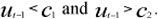
The STR model is estimated using the nonlinear least squares; however, in the LSTR model, a large g results in a steep slope of the transition function at G, thus a large number of observations is required to estimate g accurately. Furthermore, convergence of g may be slow, with relatively large changes in g having only a minor effect upon the shape of the transition function. To get around this problem, Granger and Teräsvirta (1993) and Teräsvirta (1994) proffer scaling the smoothing parameter g by the standard deviation of the transition variable, and by the variance of the transition variable in the case of ESTR (see McMillan, 2004).
4 Data discussion
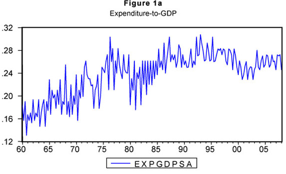
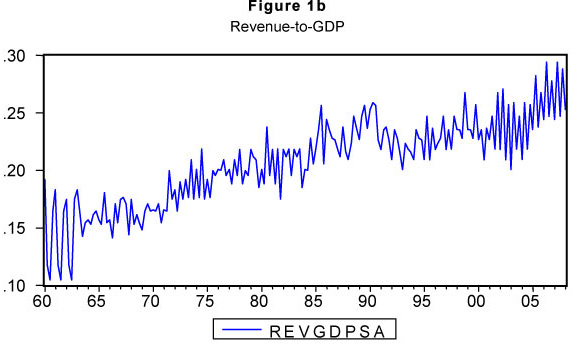
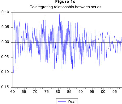
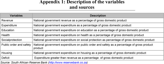
The data used to estimate the model suggested in this paper consists of the South African national government receipts and expenditures, expressed as ratios of GDP. The data, obtained from the Quarterly Bulletin published by the South African Reserve Bank, are quarterly, and seasonally adjusted, from 1960:1 to 2008:4 (see Figures 1a and b). All variables have been expressed as a percentage of GDP and converted into their natural logarithmic form. We use revenue and expenditure ratios to GDP since government authorities are mainly concerned with the dynamics of the different budget items relative to the overall size of the economy (see Hakkio & Rush, 1991; Cipollini, 2001). The cointegrating relationship between the two variables is also shown in Figure 1c.
5 Empirical results
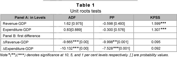
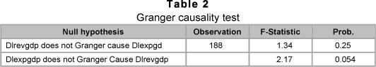
The Augmented Dickey-Fuller (1981) and Phillips-Perron (1988) unit root tests as well as the Kwiatkowski-Phillips-Schmidt-Shin (1992) stationarity tests for both series are reported in Table 1. We note that the null of a unit root cannot be rejected on the basis of Augmented Dickey-Fuller (1981) and Phillips-Perron (1988) for both series. This result is supported by the Kwiatkowski-Phillips-Schmidt-Shin (1992) test as this test rejects the null of stationarity for both series. There is no ambiguity in the order of integration; therefore we use the first differences of the series in our study. The Granger Causality test (see Table 2) gives an indication of a unidirectional causality from expenditure to taxes, i.e. supports the expenditure dominance hypothesis, implying that in South Africa budget developments are mainly determined by government spending.6 A residual-based test of cointegration as suggested by Engle and Granger (1987) and the likelihood ratio test introduced by Johansen (1991) show evidence of a long-run relation between the two variables of interest (Fig.1c).
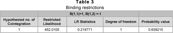
We test the hypothesis that the co-integrating vector is (1, -1). Since the p-value is not significant at the conventional levels we cannot reject the null hypothesis that the restrictions are binding (see Table 3), implying that during the sample period, fiscal policy in South Africa, consistent with the intertemporal condition of sustainability, was sustainable.
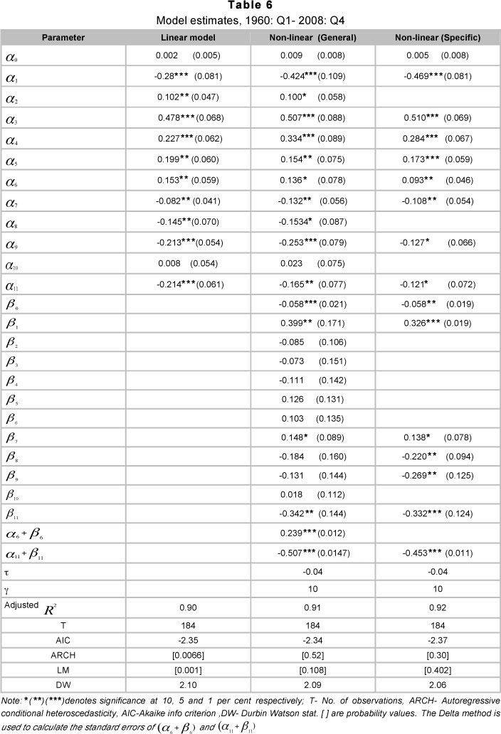
The fitted linear conditional error-correction model for revenue to GDP is shown in Table 6, column 1. The linear model seems quite satisfactory, with the post-estimation residual tests indicating normality but with evidence of heteroscedasticity. The LM-tests reject the null of no serial correlation. It may be that these significant test values are caused by neglected non-linearity (Van Dijk et al., 2002).
5.1 Linearity testing and model selection
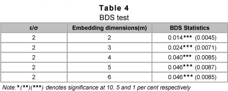
We carry out the Brock-Dechert-Scheinkman (1987) test on a series of estimated residuals to check whether the residuals are independent and identically distributed; i.e. whether the residuals from our linear model has any non- linear dependence in the series after the linear model has been fitted. Table 4 indicates that all the test statistics are significantly greater than the critical values. Thus, we should reject the null hypothesis of independent and identically distributed series/variables. The results strongly suggest that the time series in our model are non-linearly dependent, which is one of the indications of chaotic behaviour.
We also consider a parametric test, the Escribano and Jorda (EJ hereafter) (2001) linearity LM test. The null hypothesis in this test, H0, is that the series follows a stationary linear process. The computation of the test is carried out using the F- version, which is an asymptotic Wald test.
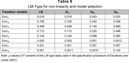
Computing the LM-type test statistics, and setting delay variable (d) equal to 1 through 8, it is seen that linearity is rejected for d =1, 2, 6 and 8 at the 5 per cent level of significance. But given that d = 6 has the smallest p-value, we select it as the delay variable (see Table 5). This implies that in South Africa it takes 6 quarters or one and a half years for fiscal policy changes to be effective.
This is not uncommon, as fiscal policy issues require legislature procedures, which take time. Deciding between the transition functions can be done by a short sequence of tests nested within H0. This testing is motivated by the observation that if a logistics alternative is appropriate, the second-order derivative in the Taylor expansion (8b) is zero (see Van Dijk & Franses, 1997). The null hypothesis to be tested is as follows:

Granger and Teräsvirta (1993) suggest carrying out all three tests, independent of rejection or acceptance of the first or second test, and using the outcomes to select the appropriate transition function. The decision rule is to select an exponential STR function only if the p-value corresponding to H02 is the smallest, and select the logistic function in all other cases. Table 5 shows that at d = 6, the logistic representation of the data is the most preferred.
5.2 LSTECM estimation
Having established a non-linear relationship we now estimate the parameters of the LSTECM by using the non-linear least squares (NLS) technique. Two LSTECM models are fitted, one is general and the other is fitted after parameter reduction (see Table 6, columns 3 and 4); this is obtained by removing the insignificant coefficients. The model estimated is specified as:
![]()
where the weight F is modelled as follows:

The parameter g which determines the smoothness of the transition regime is set at 10; and the threshold is computed to be at 0.04. As stated earlier, the delay variable (d) is computed to be at 6 quarters, i.e. one and a half years. We also follow Granger and Terävirta (1993) and Teräsvirta (1994) in making g dimension-free by dividing it by the standard deviation ofσ ecmt-d. As the surplus grows larger, ecmt-d → ∞ F → 1. As the budget deficit grows increasingly larger, ecmt-d → -∞, F → 0. When F → 0 implying (1- F) = 1, i.e. a budget deficit, the relevant parameters are a summation over a and b.
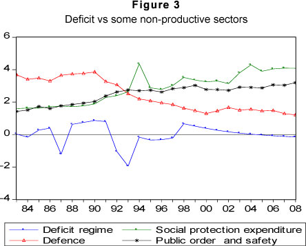
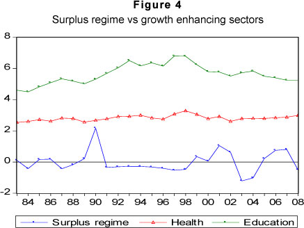
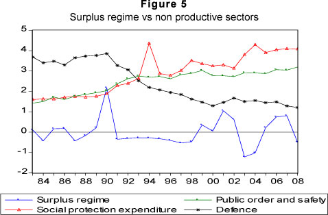
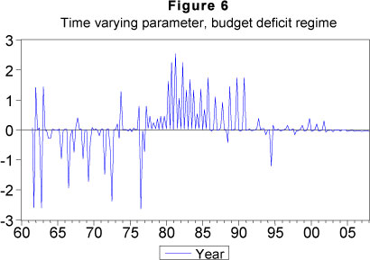
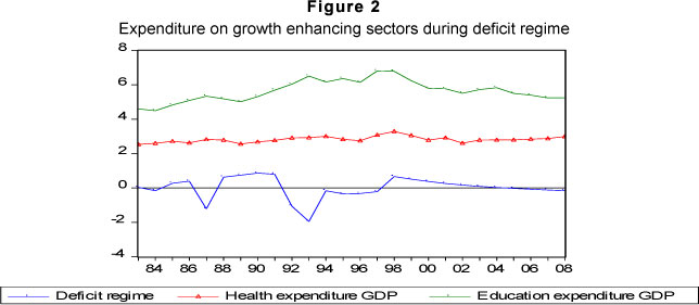
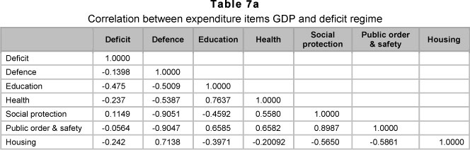
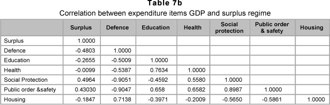
The results from estimating model equation (13) are presented in Table 6. Table 6 columns 3 and 4 report the non-linear least square estimates of our models. Tests of the residuals show no residual autocorrelation, no serial correlation, no non-normality of residuals and, finally, no heteroscedasticity. The Akaike information criterion shows that the non-linear model (i.e. model 3) is a better fit than the linear model. The error-correction terms are of the expected signs and statistically significant and show that the adjustment process to equilibrium is faster when the government budget is in deficit than in surplus. In short, y >0 government authorities are likely to react more quickly when the budget deficit exceeds 4 per cent of GDP, since it will create concern for the achievement of fiscal sustainability. The one-and-a-half-year reaction delay (i.e. d = 6) combined with a relatively smooth switch from one regime to the other g =10, can be explained in terms of the political-institutional processes (see Cipollini, 2001). Fiscal laws and regulations are drafted, through a budget document, and tabled to parliament for approval before implementation, a process that could be time consuming. The empirical result shows that a 1 percent increase in the government budget deficit (the transition variable) implies variation in the transition function that is larger (i.e. a stronger policy maker reaction) than the corresponding 1 per cent increase in a budget surplus,7 showing that in this phase the South African government becomes more concerned about solvency or fiscal sustainability. However, it appears that fiscal sustainability in South Africa has been attained at the expense of a reduction in the ratio of expenditure to GDP on education, and a relatively constant ratio of expenditure to GDP on health, during the deficit and surplus fiscal regimes (see Figures 2 and 4). Whilst the ratio of expenditure to GDP on these sectors were declining both during the budget deficit and surplus regimes, expenditure to GDP on social protection and public order and safety increased in both regimes (see Figures 3 and 5). This result is supported by the negative correlation between the thresholds (i.e. budget deficit and surplus regimes) and the trend of education and health expenditure to GDP (see Tables 7a and b). A priori one would expect that such a decline in the allocations to sectors which could stimulate growth and which in turn could generate future revenue, may pose a threat to the accumulated fiscal space.8
6 Summary and conclusion
This paper has tested the asymmetry relationship between revenue and expenditure, by making a distinction between adjustment of positive (budget surplus) and negative (budget deficit) deviations from equilibrium. It uses quarterly data on South Africa. Our findings suggest that fiscal policy over the sampled period has been sustainable, since the historical processes in South Africa are consistent with the inter-temporal government budget constraint. Of more importance, our findings show that the assumption that adjustment towards equilibrium is always present and of the same strength under all circumstances, is not valid in the case of fiscal data on South Africa.
Results from the study also reveal that government authorities are likely to react more quickly when the budget is in deficit than when in surplus, implying that the South African government becomes more concerned about solvency or fiscal sustainability in the case of the former. This adjustment could be prone to social shock, as trend expenditure on education and health to GDP has been on a decline over this period of fiscal solvency. We note, however, that what the paper has presented is to flag some important concern that may require further investigation. The authors have the intention to investigate in detail, in one of the follow-up papers, the effect of government expenditure changes and even tax policy changes that have brought about fiscal sustainability, on the economy's performance. We intend using a Dynamic General Equilibrium Model (DSGE) to investigate the impact of spending cuts on important issues such as education and health and also to assess the impact of tax cuts on the economy.
Endnotes
1 Fiscal balance as a percentage of GDP recorded 6.8 per cent in 1993.
2 Averages are calculated by the authors using data from the Reserve Bank of South Africa online historical data
3 See Burger and Fourier, 2004.
4 Although in nominal terms allocations have increased in the case of social services, like health and education.
5 See Tsay (2005).
6 The authors recognise that Granger causality is different from a test for exogeneity (Enders, 2004). Whilst exogeneity of one variable, say, expenditure, means that it is not affected by contemporaneous values of the remaining variables (taxes, debt, etc), Granger causality refers only to the effects of past values of those variables on the current value of expenditure. Our causality result reported only gives an indication of the relationship which is not firmed, because it is not the focus of the paper. Studies have shown that causality amongst variables is highly sensitive to the methodologies used, choice of variables, the frequency of the data, and the sample period (see Ndahiriwe & Gupta, 2007).
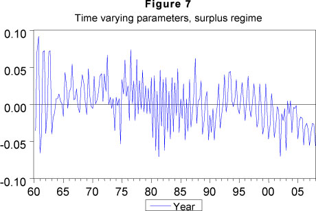
7 Figures 6 and 7 shows the state dependent speed of adjustment over time.
8 This hypothesis, however, requires further investigation.
References
BAHARUMSHAH, A.Z. & LAU, E. 2007. Regime changes and the sustainability of fiscal imbalance in East Asian countries. Economic Modelling, 24:878-89. Available online at: www.sciencedirect.com. [ Links ]
BROCK, W.A., DECHERT, W. & SCHEINKMAN, J. 1987. A test for independence based on the correlation dimension. Working Paper, University of Wisconsin at Madison, University of Houston and University of Chicago. [ Links ]
BURGER, P. & FOURIER, F.C. 2004. Sustainable fiscal policy and economic stability: theory and practice. Edward Elgar Publishing. [ Links ]
CANER, S. & SCHOEMAN, N.J. 2006. The effect of taxation on the growth of employment in the underground economy in South Africa. International Journal of Economic Studies. Also available online at www.bilkent.edu.tr. [ Links ]
CIPOLLINI, A. 2001. Testing for government intertemporal solvency, a smooth transition error correction model approach. The Manchester School, 69:643-655. [ Links ]
CRONJE, A. 1995. Deficit financing and the public debt in South Africa. Discussion Paper Series, No.2, the Budget Project. Cape Town: University of Cape Town, School of Economics. [ Links ]
CUNADO, J., GIL-ALANA, L.A. & PEREZ DE GRACIA, F. 2004. Is the US fiscal deficit sustainable? A fractionally integrated approach. Journal of Economics and Business, Elsevier, 56(6):501-526. [ Links ]
DICKEY, D.A. & FULLER, W.A. 1981. Likelihood ratio tests for autoregressive time series with a unit root. Econometrica, 49:1057-1072. [ Links ]
DWYER, G.P., LOCKE, P.R. & YU, W. 1996. Index arbitrage and nonlinear dynamics between the S&P 500 futures and cash. Review of Financial Studies. Oxford University Press for Society and Financial Studies, 9(1):301-332. [ Links ]
ENGLE, R.F. & GRANGER, C.W.J. 1987. Co-integration and error correction: representation, estimation and testing. Econometrica, 55:251-276. [ Links ]
ESCRIBANO, A. & JORDA, O. 2001. Testing nonlinearity: decision rules for selecting between logistic and exponential STAR models. Spanish Economic Review, 3(3):193-209. [ Links ]
GRANGER, C. & TERÄSVIRTA, T. 1993. Modelling nonlinear economic relationships. London Oxford Economic Press. [ Links ]
HAKKIO, C.S. & RUSH, M. 1991. Is the budget deficit 'too large' Economic Inquiry, 29:425-429. [ Links ]
HAMILTON, J.D. & FLAVIN, M.A. 1986. On the limitations of government borrowing: a framework for empirical testing. American Economic Review, 76:808-819. [ Links ]
HANSEN, G. & KIM, J.R. 1996. Nonlinear cointegration analysis of German unemployment, mimeo, Institute of Statistics and Econometrics, Christian Albrecht University. [ Links ]
HAUG, E. 1995. Has the federal deficit policy changed in recent years? Economic Inquiry, 33(11):104-118. [ Links ]
JOHANSEN, S. 1991. Estimation and hypothesis testing of cointegration vectors in Gaussian vector autoregressive models. Econometrica, 59:1551-1580. [ Links ]
JANSEN, E.S. & TERÄSVIRTA, T. 1996. Testing parameter constancy and super exogeneity in econometric equations. Oxford Bulletin of Economic and Statistics, 58(4):735-765. [ Links ]
KUNST, R.M. 1992. Dynamic patterns in interest rates: threshold cointegration with ARCH. Working Paper, Institute of Advanced Studies, Vienna. [ Links ]
KUNST, R.M. 1995. Determining long-run equilibrium structures in bivariate threshold autoregressions: a multiple decision approach. Working Paper, Institute of Advanced Studies Vienna. [ Links ]
KWIATKOWSKI, D., PHILLIPS, P.C.B., SCHMIDT, P. & SHIN, Y. 1992. Testing the null hypothesis of stationary against alternative of a unit root: how sure are we that economic time series have a unit root? Journal of Econometrics, 54:159-178. [ Links ]
MARTIN, G.M. 2000. US deficit sustainability: a new approach on multiple endogenous breaks. Journal of Applied Econometrics, 15:83-105. [ Links ]
MANUEL, T. 2004. Longer term fiscal policy issues in South Africa. Paper presented at the Bureau for Economic Research 60th anniversary conference, Somerset West, 18 November 2004. [ Links ]
MCMILLAN, D.G. 2004. Non-linear error corrections: evidence for UK interest rates, The Manchester School, 72(5):1463-6786; 626-640. [ Links ]
NDAHIRIWE, K. & GUPTA, R. 2007. Temporal causality between taxes and public expenditures: the case of South Africa. University of Pretoria Working Paper: 2007-09. [ Links ]
PHILLIPS, P.C.B. & PERRON, P. 1988. Testing for unit root in time series regression. Biometrika, 75:335-346. [ Links ]
PHILLIPS, P.C.B. & OULIARIS. 1990. Asymptotic properties of residual based tests for cointegration. Econometrica, 58:165-193. [ Links ]
QUINTOS, C.E. 1995. Sustainability of the deficit process with structural shifts. Journal of Business and Economic Statistics, 13:409-417. [ Links ]
ROUX, A. 1993. The public debt: a medium-term perspective. The South African Journal of Economics, 61(4):324-333. [ Links ]
SCHOEMAN, N.J. 1994. Public debt and the economy. Paper presented at the EBM Conference at RAU:28-29 November 1994. [ Links ]
SWANSON, N.R. 1996. Finite sample properties of a simple LM test for neglected nonlinearity in error correction regression equations. Working Paper, University of Pennsylvania. [ Links ]
TERÄSVIRTA, T. 1998. Modelling economic relationships with smooth transition regressions, in A. Ullah and D.E.A. Gilles (eds.) Handbook of applied economic statistics, New York: Marcel Dekker. [ Links ]
TERÄSVIRTA, T. 1994. Specification, estimation, and evaluation of smooth transition autoregressive models. Journal of the American Statistical Association, 89:208-218. [ Links ]
TREHAN, B. & WALSH, C.E. 1988. Common trends: the government budget constraint and revenue smoothing. Journal of Economic Dynamics and Control, 12:425-444. [ Links ]
TSAY, R.S. 2005. Analysis of financial time series (2nd ed.) University of Chicago, Graduate School of Business. [ Links ]
VAN DIJK, D. & FRANSES, P.H. 1997. Nonlinear error-correction models for interest rates in Netherlands. In W.A. Barnett, D.F. Henry, S. Hylleberg, T. Terasvirta, D. Tjiostheim and A.H. Wurtz (eds.) Nonlinear economic modelling of time series. Cambridge University Press. [ Links ]
VAN DIJK, D., TERÄSVIRTA, T. & FRANSES P.H. 2002. Smooth transition autoregressive models: a survey of recent developments. Econometric Reviews, 21(1):1-47. [ Links ]
VAN DER MERWE, E. 1994. Is South Africa in a debt trap? EPSG Occasional Paper No.6, Johannesburg: Economic Policy Group Study. [ Links ]
WILCOX, D.W. 1989. The sustainability of government deficits: implications of the present value borrowing constraint. Journal of Money, Credit and Banking, 21(3):291-306. [ Links ]
ZIVOT, D. & ANDREWS, K. 1992. Further evidence on the great crash: the oil price shocks, and the unit root hypothesis. Journal of Business and Economic Statistics,10(10):251-70. [ Links ]
Accepted: October 2011