


Serviços Personalizados
Artigo
 Africaner (pdf)
 Artigo em XML
 Referências do artigo
Indicadores

Links relacionados
-
 Citado por Google
 -
 Similares em Google
Compartilhar

 Permalink
South African Journal of Economic and Management Sciences
versão On-line ISSN 2222-3436
versão impressa ISSN 1015-8812
S. Afr. j. econ. manag. sci. vol.15 no.1 Pretoria Jan. 2012
ARTICLES
On employees' performance appraisal: the impact and treatment of the raters' effect
Temesgen Zewotir
School of Mathematics, Statistics and Computer Science, University of KwaZulu-Natal
ABSTRACT
By putting in place a performance appraisal scheme, employees who improve their work efficiency can then be rewarded, whereas corrective action can be taken against those who don't. The aim of this paper is to develop a technique that helps to measure the subjective effect that a given rater's assessment will have on the performance appraisal of a given employee, assuming that an assessment of one's work performance will have to be undertaken by a rater and that this rating is essentially a subjective one. In particular, a linear mixed modelling approach will be applied to data that comes from a South African company which has 214 employees and where an annual performance evaluation has been run. One of the main conclusions that will be drawn from this study, is that there is a very significant rater's effect that needs to be properly accounted for when rewarding employees. Without this adjustment being done, any incentive scheme, whether its motive is reward based or penalty based, will ultimately fail in its intended purpose of improving employees' overall performance.
Key words: raters' effect; performance appraisal; model diagnostics; mixed model; fixed effect; best linear unbiased predictor
JEL: C210, 49, M49
1 Introduction
Yearly performance reviews are seen as critically important for ensuring the success of public entities and private companies (Saxena, 2010). Their aim is to induce workers to become more efficient and effective (Kondrasuk, 2011), and help supervisors to become more transparent in the way they interact with their workers. As a result, workers begin to have a better understanding of their supervisors' expectations, leading to a greater sense of ownership of their duties and thus improved work performance. Ignoring these performance issues will ultimately decrease morale, which in turn will lead to a drop-off in the company's overall level of performance as management wastes time rectifying what isn't being done properly (Grote, 1996). Thus an effective performance appraisal can provide huge benefits for the employer in terms of increased staff productivity, knowledge, loyalty and participation (Margrave & Gorden, 2001).
How one best measures the performance of an employee, however, can be significantly affected by what has become known as a horns and halos effect. This refers to the effect of one person's judgment of another being unduly influenced by a first impression. A selective perception problem, the term 'horns' refers to an unfavorable first impression, while the term 'halo' refers to a favorable impression. Ideally one would like to minimise the effect that a first impression has on a final rating, but this selective perception bias has been observed in the behaviour of all raters, and is therefore known as raters' effect (Wolfe, 2004).
Due to the complexity of the job performance and interpersonal relations at work, much of the existing research typically indicates that raters account for significant proportions of the variance in employees' true performance (Woehr et al, 2005; Hoffman & Woehr, 2009; Hoffman et al, 2010). It is therefore in the interests of both the organisation and the individual to maximise the effectiveness of performance appraisal by reducing the rater errors (see for example, Aguinis & Pierce, 2008; Uggerslev & Sulsky, 2008; Ferris, 2008; Ogunfowora, 2010). Most of the studies focus on the rating strategies before the rating rather than attending to rating outcomes.
Therefore, the purpose of this study is to introduce a statistical method to (i) demonstrate the plausibility of rater source factors at the performance appraisal; (ii) to identify (and adjust for) the magnitude of raters' effect and thereby rank the 'best' and 'worst' performers, and (iii) identify deviant ratings. Hence, this study contributes to the literature by attempting to clarify the structure of raters' effect, the existence and nature of raters' effect, and the relative proportion of variance accounted for by the raters' influence on performance ratings.
2 The data and purpose of the analysis
The South African based company1 has 214 employees. All were included in the study as each employee was part of a per annum based performance appraisal scheme. For each project (or activity) in which he/she was involved, that employee was given a rating on a continuum scale ranging from 0 to 25, with a higher rating showing a better performance. The ratings were performed by 85 evaluators. The scale of complexity of the given tasks that the employees were being asked to perform was also taken into consideration when the rating was being done by the evaluators.
To help mitigate the effect of using different raters, all 85 raters received some form of training (i) to familiarise themselves with the measures that they would be working with, (ii) to ensure that they understood the sequence of steps that they would have to follow in their assessment and (iii) to explain how they should interpret any normative data that they would be given. More details about the data can be obtained from Zewotir (2001).
If one were able to use all 85 raters to rate each and every employee in the firm, raters' training would minimise rater effects, as the effects would be the same (Pulakos, 1986; Houston et.al., 1991). No single employee would run the risk of having a lower or higher overall rating as all the employees would receive the same benefit or penalty from the rater's subjective leniency or harshness. In the firm that we studied, however, not every employee was able to be rated by the same set of raters. In particular, Table 1 shows how some raters evaluated several employees whereas others only rated a few employees. It should be noted that in Table 1 there are 340 ratings of 214 employees because some employees were involved in a number of projects (or activities) and accordingly had multiple raters.
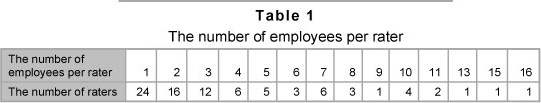
The difference between the rating that will be assigned by a single rater and the average rating that will be assigned by all 85 raters is called the 'raters' effect'. Clearly, if this raters' effect is non zero, then employees that have been evaluated by a different set of multiple raters may receive an unfair (i.e. biased) score primarily because they have faced a relatively lenient or relatively harsh set of judges when compared with the other employees in the firm. In this case, an adjustment to a given employee's average score should be made, which takes into account the potential bias that may arise because a different set of raters has been used. Simply averaging the score given by each rater to an employee will not adjust this raters' effect. In the next section we will develop a method that attempts to account for a raters' effect. Once this has been done, we can then separate 'good' performers from 'poor' performers and reward them accordingly.
3 Formulation of the model
A classical example of testing for inter-rater reliability is described by Fliess (1986) in the context of a medical situation where depressive patients are being rated by several psychiatrists, and there is a restriction on the number of examinations that a patient can undergo. However, this method cannot be used in our context of performance appraisal because the rater who is evaluating a given employee is someone who has a detailed knowledge of that person's performance, i.e. the random assignment of employees to any given evaluator is not possible in our context. Furthermore, one is not necessarily able to restrict the number of employees that each rater sees, or vice versa.
Some researchers have suggested that one calculate a mean performance score for each employee and then rank the employees based on their mean performance. As has already been noted, because the set of raters being used differs from one employee to the next, simply ranking the mean performance scores of each employee will not remove the rater bias in this procedure (Russell, 2000). Other researchers have attempted to develop an analysis of variance-based raw scores (Braun, 1988; de Gruijter, 1984; Houston et al., 1991) or a multifaceted Rasch model (Wolfe et al., 2001; Wolfe 2004). Such a model however requires that one make use of a Likert scale when rating an employee's performance (like Excellent, Very good, Good, Fair, Poor).
In our modelling context the rating that is given is not based on a Likert scale. In order to develop a performance score for a given employee and to correct this score for a possible rater's effect, we will use a linear mixed model i.e.
yij = µ + αi + βi + εij
where yij denotes the appraisal score of the ith employee that has been given by rater j, µ denotes an overall mean score, αi denotes a deviation of employee i from this overall mean score, βj denotes the jth rater's effect and εij is an error term. In particular, we will assume that the αis are independent identically distributed normal random variables with a mean 0 and variance σ12, and the εijs are independent identically distributed normal random error terms with mean 0 and variance σ02, respectively. Focusing on the model parameter βj some of the management group may want to look only at the 85 raters, in which case the raters' effect βj should be treated as being a fixed effect. On the other hand, some may argue that the 85 evaluators are representatives from a population of raters, in which case the raters' effect should be treated as being a random effect.
Instead of arguing about whether this raters' effect should be fixed or random, we will construct two models: one with a raters' effect that is fixed and another where we treat this raters' effect βj as being an independent identically distributed normal random variable with a mean 0 and variance σ22. We will also assume that αi, βj and εij are distributed independently of each other. The resulting model then becomes a linear random effects model. A detailed discussion about linear random effect models can be found in, among others, Harville (1990), Robinson (1991), Searle et al. (2006) and SAS Institute (1992). The main focus of interest in this model is the variance of the raters' effect, σ22. If σ22 = 0, then the data supports the hypothesis that the raters' effect is constant or identical. In other words, employees receive an identical bias from any rater that is assigned by the company implying that there is no need to adjust the employee's score with respect to a raters' effect. On the other hand, if the hypothesis σ22 = 0 is not supported by the data, then different raters have a different level of leniency/severity that they employ when judging an employee's performance, and thus the employee's score should be adjusted to account for this effect.
In a fixed effects model our main interest will focus on whether the βjs are identical for all j = 1, 2,...,85. Such a model is known as a two-way mixed effect (see, for example, Little et al., 2000; Skrondal & Rabe-Hesketh, 2004; McCulloch et al., 2008). If the data supports the following hypothesis H0: β1=β2=...=β85 then the employees will be receiving an identical bias from all the 85 raters so that there will be no need to adjust the employee's score for this rater's effect.
An important component of this model is a measure of its reliability. Sometimes called an intra-class correlation (ICC) coefficient, ρ, can be defined as the proportion of the total variance of the scores that can be attributed to the true performance score.
The estimation of the employee based variables ai will make use of a technique which is known as Best Linear Unbiased Prediction (BLUP). BLUP is a class of statistical tools that has some desirable properties (Robinson, 1991; SAS, 1992; Searle et al., 1996; McCulloch et al., 2008). The term "Best" in the acronym BLUP is used to describe the property that, from the available data on an employee, its predicted true performance will be as error-free as possible. The term 'linear' simply means the data has not been adjusted to some other scale such as being squared. 'Unbiasedness' means that, on average, the estimated true performance calculated will be the same as the employee's true performance. 'Prediction' refers to the task at hand: trying to predict true performance.
Once a BLUP has been obtained for each one of the employee based parameters, a hypothesis test can be constructed by noting that the standardised BLUP's are distributed as a Student's t-distribution with degrees of freedom equal to the denominator degrees of freedom (ddf). One can then pinpoint the ith employee as being a significantly good/bad performer if the standardised BLUP is greater than t(1-α/2, ddf) where t(1-α/2;ddf) is the lower 1-α/2 level of Student's t distribution with degrees of freedom ddf. For exceptionally good performers, the estimate will be positive valued and for bad performers it will be negative valued.
Model diagnostics also form an important part of statistical modelling. Zewotir and Galpin (2004, 2005 and 2007) have outlined some formal and informal procedures that can be used to help detect outliers, influential points and specific departures from underlying assumptions in the linear mixed models. These procedures will also be employed in this paper.
4 Results and discussions
4.1 Without an adjustment for the raters' effect
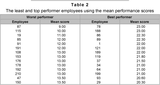
One can perform an analysis without adjusting for the raters' effect, by simply using the average score that has been assigned by all the raters to a given employee. Using this approach, the best and worst performers are presented in Table 2.
4.2 Adjusted model 1: Including a raters' effect as a fixed effect
Results for the rater fixed effects model are given in Table 3. The rater row of Table 3 is testing whether the rater effect parameter estimates that we have obtained are significantly different from zero. The very small p-value that we have obtained (p = 0.0001) indicates that the hypothesis H0: β1=β2=...=β85 = 0 can be rejected. This clearly shows the existence of a rater bias in the scores given to different employees of the firm.
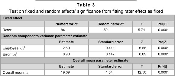
The variance parameter estimate for σ12 that is given in Table 3 indicates that there is also variability in the performance between employees that is statistically significant and therefore needs to be accounted for. In fact 73% of the total variance associated with the employees' score is attributable to the true performance score variability of the employees, σ12.
Table 4 provides a ranking of employees based on the BLUPs that have been obtained for αi. The results need to be interpreted as a continuum where large negative values indicate a poor performance and large positive values indicate an excellent performance. An estimate for each employee's true performance score can then be obtained by adding the appropriate BLUP score that has been given in Table 4 for a given employee to the overall mean estimate of 19.39 that has been given in Table 3.

Unlike the results in Table 2, the results in Table 4 account for the bias from raters and adjust the employees' score for this rater's effect. Besides the adjustment for the raters' bias, Table 4 accounts for the variability of the employee score. For instance, employee 100 was not listed as one of the poor performers in Table 2, but is listed as the second poorest performer in Table 4. When we scrutinise the evaluation report of employee 100 we see that employee 100 was rated by two raters (raters 32 and 58, with a score of 15.9 and 12.5 respectively). However, these two raters rated other employees; for example rater 32 rated eight employees and gave them scores of 18.2, 21.8, 16.6, 22.3, 20.6, 17, 19.6 and 15.9 respectively and rater 58 rated two employees with scores of 20 and 12.5 respectively. From the two raters we note that the score of employee 100 is the lowest. Moreover, by tracing back to determine how raters 32 and 58 rated other employees relative to the other raters, we note that, on average, raters 32 and 58 tended to be more lenient. With all these considerations in the model, the predicted performance score for employee 100 then becomes a significantly negative score, as given in Table 4. But the crude average score of employee 100, 14.2, would not place this employee among the worst performers. Likewise by adjusting for raters' effect employee 15 becomes one of the top performers, as shown in Table 4, whereas this employee was not listed as a top performer in Table 2.
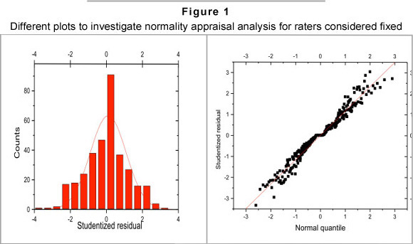
Figure 1 contains a set of plots that can be used to assess the normality assumption and the goodness of fit of the data. The plots indicate no recognisable outlier in the data. The application of a more formal test (as outlined in Zewotir & Galpin, 2007) also did not record the maximum absolute Studentised residual as being an outlier. The normal probability plot is linear, which indicates that the assumption of normality is reasonable. The linearity of the plot is also supported by the W-statistic which is an adaption of Shapiro and Wilk's (1965) normality test to a linear mixed model (Zewotir & Galpin 2004). In particular, the following result was recorded (W =0.9777 for which p=0.0665) which favours the normal distribution.
Focusing on those observations, that could be potential outliers for our study, it was found that observation numbers 123 and 246 were the most influential observations. When these observations were removed, however, no significant change in the parameter estimates or goodness of fit of the resulting model was recorded. Nevertheless, because we are dealing with people who we may want to incentivise it could be argued that one would like to examine these two outliers more carefully.
Observation number 123 contains a score of 15 for employee 72 that has been given by rater 27. This same employee was also rated by three other people (namely, raters 21, 37 and 58) who gave that employee the following respective scores (22, 18, 19.6). It should be noted that rater 27 also had to rate nine other employees and the score of employee 72 was the lowest given by rater 27. Raters 21, 37 and 58, however, put employee 72 as their 3rd, 3rd and 2nd highest performing employee, respectively.
Case number 246 deals with employee 155 who was rated by a single person (rater 35) and was given a score of 20. It should be mentioned that rater 35 also had to rate seven other employees (employees 33, 73, 87, 155, 162, 194, and 202) giving them the following respective scores (13, 15, 9, 20, 12, 18, and 15). In terms of the ratings that these seven employees received from other people, the score of rater 35 was found to be the lowest for five of these employees and the second lowest for another one of these employees. Because of this obvious downward bias in the rating record of rater 35, when an adjustment is being made to employee 155's score, the predicted performance score for employee 155 then becomes very large as reflected in Table 4.
4.3 Including a raters' effect as a random effect
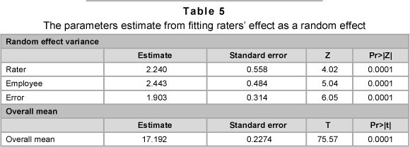
Maximum likelihood estimates for the model parameters and the associated tests of significance are presented in Table 5. The results indicate that the rater and employee effects are significant.
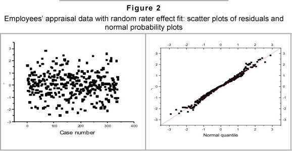
Employing our formal outlier testing procedure does not label any observation as being an outlier. A graph of the residuals is given in Figure 2. None of the observations appear to be separated from the bulk of other observations. The normal probability plot does not indicate a serious violation of the normality assumption. The summary statistic (W = 0.978), also favours a normality assumption (p = 0.0860).
A prediction of the true performance of each employee shows that ten employees (see Table 6) can be regarded as performing exceptionally badly or well. For exceptionally good performers, note that the estimate will be positive-valued and for bad performers the estimate will be negative-valued. Furthermore, the prediction of an employee's true performance is obtained by adding the estimate given in Table 6 to the overall mean that we obtained for the model.
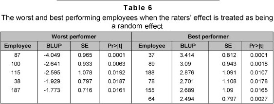
All the worst and best performers given in Table 6 were also identified as the worst and best performers in Table 4. The consistency of the employee's performance and the overall variability in the harshness and leniency shown by the 85 raters, were the only role players in Table 6 results. But the role players for Table 4 results were the average leniency or harshness of the raters who rated the employees and the employees' performance. Since employees who were rated by fewer raters have a less consistent performance predictor, the majority of the worst or best performers who were rated by only one rater were the least favoured to be listed from Table 4 into Table 6. For instance, consider employees 37 and 86 from the top performer employees given in Table 4. Employee 37 was rated by three raters with a score of 21, 22 and 22. On the other hand, employee 86 was rated by a single rater with a score of 22.3. Employee 35 is a consistent performer and leads the top performers in Table 6, but not so employee 86.
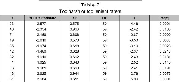
Since the raters' effects were considered as random effects, we obtain the BLUP estimate of the realised raters' effect. An investigation of these estimates of the BLUPs of raters' effect showed the harshness or leniency displayed by raters in their judgments. Table 7 provides the extreme rankings of raters based on the BLUP's estimate of the raters' effect latent values: large negative values indicate a harsh rater and large positive values indicate a lenient rater. Rater 23, who evaluated thirteen employees and gave them the following scores 11, 19, 18, 12, 15, 16, 12, 15, 10, 14, 16, 14 and 13, can be viewed as being the most harsh rater. Similarly, rater 31, who evaluated 6 employees and gave them the following scores 21, 21, 24, 22, 22 and 21, can be viewed as being the most lenient rater.
With regard to the existence of some possibly influential observations, observations number 69 and 297 were flagged in the analysis. Omitting both cases from the analysis did not substantially change the estimates that we obtained for the variance parameters or the overall goodness of fit of the model. It is interesting to note, however, that case 69 represents a score of 24 that was given to employee 39 by rater 43. This score was in fact the largest score that was given by any one rater to any one employee. The next highest score received by an employee was 16, which resulted in rater 43 being flagged an outlying rater in Table 7.
Case 297 refers to a score of 23 for employee 188, given by rater 40. This score is the second highest score that was given by a rater in the entire employees' evaluation process. Furthermore, this was the only score that employee 188 received.
In Table 2, results were based on the crude average scores without any consideration of adjustment for the raters' effect. In Table 4 the employee performance predictor takes the average leniency/harshness of the associated rater into consideration. In Table 5 the consistency of the employee in the ratings, is taken into account. What is evident from Tables 2, 4 and 6 is that the interest is in the true performance of the employee not in an average score based on a few measures/rates about the employee's performance. The basic problem is that the observed value on the employee is not equal to the employee's true performance. How should we then estimate an employee's true performance latent value? The mixed model random effect links the rating to the true performance latent value. The estimate of the employee-true performance latent value is typically the BLUP estimate. As the number of measures on an employee gets larger, the BLUP estimate becomes consistent and approaches the employee's true performance latent value. The results in Tables 4 and 6 are sufficiently convincing to use the BLUP estimates in employees' appraisal routine practice by considering raters' effect as fixed or random.
5 Conclusions and implications
Performance appraisal systems are essential for a company to run efficiently and productively. With performance appraisal in place, employees can be given a sense of ownership and responsibility with regard to the duties that they perform. The challenge is to know how best to adjust a given measure of an employee's performance so that it is not unduly influenced by a rater's tendency to make private and highly subjective assessments. Using a simple average of scores from a set of raters will not adjust for any hidden subjectivity that may reside in that specific group of raters. Because different employees are being assessed by different raters, a subjective bias may be introduced into the rating of one employee when compared with that of another employee. This paper has sought to address this problem.
The linear mixed model that has been applied in this study allows for some flexibility with regard to whether one wants to view a rater's effect as being a fixed or random effect. A rater effect can be treated as being fixed if the raters are being selected by the company with the purpose of comparing one rater with another. On the other hand, the raters' effect can be treated as being random if we want to make statements about the variation in the overall population from which our raters are being drawn.
Because we are interested in effects that, we believe, are common to all individuals and also effects that are different among individuals, a mixed effects model can be used to capture both these features. The mixed model provides estimates (BLUPs) of each employee's true performance which can then be subjected to a formal test to identify those employees who, statistically, are significantly good or bad performers in the company.
The model's diagnostics tools that we have used help to provide some reassurance that the model is not being contradicted by the data that we are observing or is being unduly influenced by particular characteristics of the data. The results of this paper have consistently shown that, unless the same raters are evaluating all employees, there are considerable rater based effects which cannot simply be ignored in any employees' performance appraisal.
Acknowledgement
The author is grateful to the anonymous reviewers and the managing editor for several important comments and suggestions. The author is also grateful to Prof Michael Murray and Dr Edilegnaw Wale for their careful reading of the first draft.
References
AGUINIS, H. & PIERCE, C.A. 2008. Enhancing the relevance of organizational behavior by embracing performance management research. Journal of Organizational Behavior, 29:139-145 (2008). [ Links ]
BRAUN, H.I. 1988. Understanding score reliability: experiments in calibrating essay readers. Journal of Educational Statistics, 13:1 -18. [ Links ]
DE GRUIJTER, D.N 1984. Two simple models for rater effects. Applied Psychological Measurement, 8: 213-218. [ Links ]
FERRIS, G.R., MUNYON, T.P., BASIK, K., & BUCKLEY, M.R. 2008. The performance evaluation context: Social, emotional, cognitive, political, and relationship components. Human Resource Management Review, 18:146-163. [ Links ]
FLEISS, J.L. 1986. Design and analysis of clinical experiments. New York: John Wiley & Sons. [ Links ]
GROTE, R.C. 1996. The complete guide to performance appraisal. New York: AMACOM, AMA's book publishing division. [ Links ]
HARVILLE, D.A. 1990. BLUP (Best Linear Unbiased Prediction) and beyond. In advances in statistical methods for genetic improvement of livestock, 239-276. New York: Springer-Verlag. [ Links ]
HOFFMAN, B. & WOEHR, D.J. 2009. Disentangling the meaning of multisource feedback source and dimension factors. Personnel Psychology, 62.735-765. [ Links ]
Hoffman, B.J., Lance, C, Bynum, B., & Gentry, B (2010). Rater source effects are alive and well after all. Personnel Psychology, 63:119-151. [ Links ]
HOUSTON, W.M., RAYMOND, M.R. & SVEC,J.C. 1991. Adjustments for rater effects. Applied Psychological Measurement, 15(4):409-421. [ Links ]
KONDRASUK, J.N. 2011. So what would an ideal performance appraisal look like? Journal of Applied Business and Economics, 12(1):57-71. [ Links ]
LITTLE, T.D., SCHNABEL, K.U. & BAUMERT, J. 2000. Modeling longitudinal and multilevel data. London: Lawrence Erlbaum Associates Publishers. [ Links ]
MARGRAVE, A. & GORDEN, R. 2001. The complete idiot's guide to performance appraisals. New York: Alpha Books/Macmillan. [ Links ]
McCULLOCH, CE. SEARLE, S.R., & CASELLA, G. 1996. Variance components. New York: John Wiley. [ Links ]
McCULLOCH, CE., SEARLE, S.R. &NEUHAUS, J.M. 2008. Generalized, linear, and mixed models (2nd ed.) New York: John Wiley. [ Links ]
OGUNFOWORA, B., BOURDAGE, J. & LEE, K. 2010. Rater personality and performance dimension weighting in making overall performance judgments. Journal of Business and Psychology, 25:465-476. [ Links ]
PULAKOS, E.D. 1986. The development of training programs to increase accuracy on different rating forms. Organizational Behavior and Human Decision Processes, 38:76-91. [ Links ]
ROBINSON, G.K. 1991. That BLUP is a good thing: the estimation of random effects. Statistical Science, 6: 15-51. [ Links ]
RUSSELL, M. 2000. Summarizing change in test scores: shortcomings of three common methods. Practical Assessment, Research & Evaluation, 7(5). Available at: http://pareonline.net/getvn.asp?v=7&n=5 [Accessed 2009-09-16]. [ Links ]
SAS INSTITUTE 1992. SAS Technical Report P-229. Carey (North Carolina): SAS Institute Inc. [ Links ]
SAXENA, S. 2010. Performance management system. Global Journal of Management and Business Research, 10(5):27-30. [ Links ]
SHAPIRO, S.S. AND WILK, M.B. 1965. An analysis of variance tests for normality (Complete Samples). Biometrika, 52:591-611. [ Links ]
SKRONDAL, A. & RABE-HESKETH, S. 2004. Generalized latent variable modelling: multilevel, longitudinal and structural equation models. London: Chapman and Halls. [ Links ]
UGGERSLEV, K.L., & SULSKY, L.M. 2008. Using frame-of-reference training to understand the implications of rater idiosyncrasy for rating accuracy. Journal of Applied Psychology, 93:711-719. [ Links ]
WOEHR D.J., SHEEHAN, M.K., BENNETT, W. 2005. Assessing measurement equivalence across ratings sources: a multitrait-multirater approach. Journal of Applied Psychology, 90:592-600. [ Links ]
WOLFE, E.W. 2004. Identifying rater effects using latent trait models. Psychology Science, 46:35-51. [ Links ]
WOLFE, E.W., MOULDER, B.C., & MYFORD, C.M. 2001. Detecting differential rater functioning over time (DRIFT) using a Rasch multi-faceted rating scale model. Journal of Applied Measurement, 2:256-280. [ Links ]
ZEWOTIR, T. 2001. Influence diagnostics in mixed models. PhD thesis: University of Witwatersrand. [ Links ]
ZEWOTIR T. & GALPIN, J.S. 2004. The behaviour of normality under non-normality for mixed models. South African Statistical Journal, 38:115-138. [ Links ]
Accepted: September 2011
1 The name of the company could not be disclosed for anonymity reasons.

