RESEARCH ARTICLES

 

Risky localities: Measuring socioeconomic characteristics of high murder areas

 

 

Lizette Lancaster^I; Ellen Kamman^II

^IManages the South African Crime and Justice Information and Analysis Hub of the Institute for Security Studies' (ISS) Governance, Crime and Justice Division. Her focus is the collection, analysis and dissemination of data and information to promote evidence-based crime and violence reduction policies and strategies. llancaster@issafrica.org
^IIHas a MA in Biomedical Health Sciences. She is an independent consultant and has been involved in data analysis for organisations such as the ISS. ellen@absamail.co.za

 

 

---

ABSTRACT

Every day, on average, more than 49 people are murdered in South Africa. A better understanding of the demographics of locations with high murder and other crime rates could assist the development of initiatives to reduce them. It could also provide the basis for research into how social structures and relationships affect violence reduction. This article explores the hypothesis that the risk of murder is associated with certain demographic characteristics in particular locations. It proposes a method for analysing the demographic characteristics of police precincts in relation to the murder rate, and provides a summary of initial results. The article concludes with a discussion on the usefulness and limitations of this approach.

---

 

 

Theoretical framework

South Africa's high violent crime rates are predominantly the result of interpersonal violence perpetrated by people who know each other.¹Various researchers have explored these trends in relation to the Chicago School's social ecological approach to understanding crime, and subsequent theories of social disorganisation.²

Shaw and McKay were among the first to introduce a scientific method to address problems of social control and disorganisation. Social disorganisation, they suggested, occurs where social control is weak, because conventional institutions of social control (such as family structure, schools, churches and voluntary community organisations) are incapable or unable to 'order' the behaviour of the community's youth.³

Abbott summarises the Chicago School's social ecological approach by noting 'that one cannot understand social life without understanding the arrangements of particular social actors in particular social times and places ... [N]o social fact makes any sense abstracted from its context in social (and often geographic) space and social time. Social facts are located facts. [emphasis in original]'⁴

Furthermore, crime is not evenly distributed across all locations.⁵ For this reason, Chicago School scholars such as Park, Burgess and McKenzie were the first to combine qualitative and quantitative research methods to understand the social dynamics of communities in particular locations.⁶

Shaw and McKay concluded that low economic status, ethnic heterogeneity and residential mobility are three structural factors that have a negative impact on social disorganisation and could, in turn, account for variations in delinquency and crime.

Sampson and Groves note that while the testing of macro-level characteristics such as median income from census data could generate a useful preliminary test, it does not provide the variables required to measure, among others, the impact of community structures and relationships on crime.⁷ It is therefore important to note that a comprehensive analysis of risk factors will require multiple datasets in addition to crime and census data.

Using victimisation data in addition to administrative data, Sampson and Groves extended the structural factors identified by Shaw and McKay to include family disruption and urbanisation. They also expanded the theoretical framework to include intervening mechanisms such as 'sparse local friendship networks', 'unsupervised teenage peer groups' and 'low organisational participation'.⁸

Subsequent studies on social disorganisation link structural factors to delinquency as well as property and violent crime, to varying degrees. Poverty and economic deprivation are strongly associated.⁹

The drivers of interpersonal violence based on the social ecological framework are best summarised by the ecological model adopted by the World Health Organization (WHO).¹⁰ Here, interpersonal violence is regarded as the result of a combination of multi-level factors related to the individual, relationships, the community and society. The ecological framework is outlined in Figure 1.

 

 

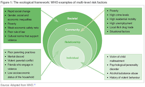
Therefore, the predictors of murder and other violent crimes are interrelated, requiring multi-stage interrogation and analysis. As such it is important to study the impact of such factors on crime and violence rates in stages, using different data sets and utilising multiple methods.

This article provides a description of the first steps one might follow in initiating an interrogation of the risk factors contained in the community and societal spheres of Figure 1, with the appropriate variables available in the South African census. The exploratory analysis undertaken here is purely intended for illustrative purposes, aiming to highlight the possible uses for the linked data. Comparing areas with high murder rates can provide helpful insights into the level of risk of murder in different communities in South Africa.

 

Current available crime data

On an average day more than 49 people are murdered in South Africa.¹² Since 2013 the murder rate has increased by 9.2% from 30 murders per 100 000 to 32.9.¹³

Currently, the most accessible figures available on murder are the South African Police Service's (SAPS) crime statistics. The SAPS releases its recorded crime statistics annually (usually in September) for the previous financial year (April of the previous year to March of the release year). Among the 29 different crime and violence categories, the SAPS provides murder statistics for the country, for each province, and for all 1 139 police station precincts.

Crime rates (per 100 000 population) are made available on a provincial and national level. While this enables comparisons across the provinces, it gives very little information about the differences between local level areas and so-called 'crime hotspots'. A crime hotspot is regarded by Eck et al. as 'an area that has a greater than average number of criminal or disorder events, or an area where people have a higher than average risk of victimization'.¹⁴

The precinct level murder figures provided by the SAPS have many limitations. Among others, only raw figures are provided, without any correction for the size of the population in the precinct. This means that the murder risks across precincts cannot be compared because the size of the population can be very different. One precinct may consist of 5 000 inhabitants while the neighbouring precinct may have 60 000 inhabitants. Furthermore, the specific location of criminal incidents within the precinct is not provided.

Statistics South Africa (Stats SA) can provide information about the number of households and the number of individuals per municipal ward, but these boundaries do not coincide with the SAPS precinct boundaries. This makes it difficult to link the census data to the crime statistics at a local level, so as to get a better understanding of comparative crime rates per 100 000 population. However, the Institute for Security Studies (ISS) has developed a method for providing this type of analysis. The following section gives a detailed explanation of this methodology.

 

Aim of the study

Using murder rates per 100 000 population allows for comparisons of locales with the highest risk of murder, and between different precincts.

This study explores the hypothesis that the risk of murder is associated with certain demographic characteristics in particular locations. To do this, a three-fold process was used:

1. Estimating population size per police precinct and linking census data

2. Calculating crime rates

3. Undertaking multiple regression analysis

The section below contains a discussion of the methodology followed to undertake this process.

 

Methodology

Estimating population per precinct and linking census data

To provide an estimation for the number of households and the number of individuals living in each precinct, the ISS developed a methodology whereby Stats SA's small area data from the 2011 census and the police precinct boundaries released by the SAPS are projected onto each other, creating polygons. Small areas are units of analysis provided by Stats SA to allow for in-depth analysis of census data. With the release of the Small Area Layer (SAL) level of data from the 2011 census, it becomes possible to provide an estimate of the population per precinct.

In areas with high population density, the surface area of the unit of analysis will be small, as the areas are based on a rough estimate of the number of households. In sparsely populated areas, the area covered by this unit of analysis may therefore be much larger.

Overlaying the spatial data from the 2011 census with precinct boundary data provided by the SAPS, 96% of the SAL units fall completely within the boundaries of a police precinct. Figure 2 gives an example of the overlay of precinct boundaries (green lines) with the SAL layer. The population data and household census data for the areas that fall completely within the precinct boundaries are assigned to that police station.

 

 

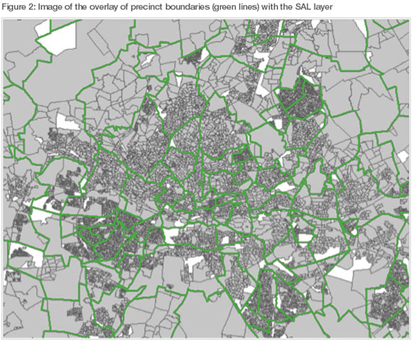
For the remaining 4% of SAL areas, a very basic area proportional assignment was used. For example, if 30% of small area X falls within precinct A and 70% within precinct B, 30% of the population and all related census data are allocated to precinct A, and 70% of the population is allocated to precinct B. Adding up all the small areas and partial small areas within each precinct then gives us an estimated population per precinct.

Each year, Stats SA releases mid-year population estimates at a provincial and district municipality level. The population estimates per police station are updated each year, using the district level population growth estimates provided by Stats SA in the mid-year population estimates. This growth rate is then applied to all the precincts in that district.¹⁵

Calculating crime rates

To calculate the crime rates for each police precinct, the number of crimes per precinct from the 2014/2015 SAPS crime statistics are divided by the population per precinct. The total is multiplied by 100 000 to derive the crime rate per 100 000 population.

Multiple regression analysis

The data were analysed using multiple linear regression utilising SPSS 23 statistical software. Linear regression is used to predict the influence of various input variables (independent variables) on one output variable (dependent variable). Various models were tested to ensure minimal collinearity between the independent variables in each model. The independent variables and dependent variables are described below.

Independent variables

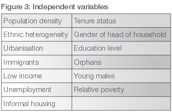
Several independent variables were identified in the initial and exploratory research based on the ecological framework, as they provided insight into the individual, relationship, community and societal characteristics of the population in each precinct. As our analysis is limited to data from the 2011 census, the indicators below were used in the regression models.¹⁶ These indicators could be used to approximate the different layers of risk factors mentioned in the ecological framework model. The selected variables are summarised in Figure 3 and a detailed description is provided in the text.

 

 

Population density

Population density was calculated using the population estimates per precinct as calculated for 2014/2015, divided by the surface area of the precinct in km² according to the SAPS precinct boundary data. The population density for South Africa is estimated at 43 people per km².

Ethnic heterogeneity index

Sampson et al. theorise that ethnic heterogeneity as a measure of social disorganisation can influence certain types of crime in a specific area.¹⁷ A commonly used measure for heterogeneity is the heterogeneity index described by Blau.¹⁸ The index is calculated on the population group variable, and is described by where pi is the fraction of the population in a given group. This measure increases when heterogeneity increases, and is zero when there is no heterogeneity (for example, when only one population group is present).

Proportion urban

Census 2011 provides the variable geotype. The proportion urban variable was calculated by dividing the number of people living in urban geotype areas by the total number of people in the precinct.

Proportion immigrants

The proportion of immigrants in each precinct was calculated using the migration questions from the 2011 census. Each person in the household was asked whether they stayed in the same area 10 years before and, if they had moved into the area within the last 10 years, they were asked for their country or province of origin. If they were from outside South Africa, they were classified as 'immigrant'.

Proportion low income

Monthly household income is used as an indicator of household level poverty. Many households survive on social grants, including child support grants and old age pensions. The proportion of households in a police precinct with a total monthly household income below R1 600 per month¹⁹ was calculated to give an indication of poverty.

Proportion unemployed

Using the labour force data from Census 2011, the proportion of unemployed people in the labour force (ages 15-65) was calculated per precinct.

Proportion informal

The number of households living in informal dwellings was calculated relative to the total number of households.

Proportion renting

The number of households renting their dwelling was calculated relative to the total number of households.

Proportion female head of household

The number of households headed by females was calculated as a proportion of the total number of households in the area.

Proportion low education

To estimate the number of people with no or limited education, the total number of people with primary school education or less (up to and including Grade 7) was calculated as a proportion of the total number of people in the area.

Proportion orphans

The percentage of orphans was determined by calculating the number of children under the age of 20 whose mother is not alive, as a percentage of the total population.

Proportion young males

The percentage of young males was calculated by dividing the number of males between the ages of 18 and 35 by the total population.

Relative poverty

To estimate the relative poverty of a precinct compared to surrounding areas, the average income was calculated for each precinct and municipality. Relative poverty is the average municipality income divided by the average precinct income. A high value for this indicator implies that the municipality average income is relatively high compared to the precinct average income, and the precinct population is relatively poor when compared to the rest of the municipality. A low value for this indicator implies that the precinct average income is relatively high compared to the rest of the municipality.

Dependent variables

The initial focus of the research was to identify socioeconomic indicators, which could help predict the murder rate at a precinct level. During this analysis it became clear that the murder rate at a precinct level fluctuates heavily in the smaller precincts, creating unwanted outliers in the data. These outliers are more pronounced in the precincts with smaller populations, and these were excluded from the analysis.

The fluctuations are less pronounced if the average murder rate over 10 years is applied to the model, and a further analysis was done using this dependent variable.

One of the conditions of multiple regression models is that the residual values have to follow a normal distribution. For the dependent variables used in this model, this is not the case. A common transformation applied to the data is log transformation. The natural log value of each dependent variable is entered into the model instead of the value. After this transformation, the residual values follow a normal distribution.

Murder rate

The murder rate was calculated by dividing the number of murders in the precinct in the 2014/2015 year of analysis by the total population of that precinct in 2014/2015, and is reflected as the number of murders per 100 000 people. Precincts with an estimated population below 20 000 are excluded from this analysis.

Murder rate average over 10 years

In smaller precincts, the murder rate per 100 000 population will fluctuate drastically, even when the actual number of murders remains small. For this reason, the average number of murders was calculated for the last 10 years, and then divided by the current population. This will lead to less obvious fluctuations in the murder rate, especially in the smaller precincts, and all precincts are included in this analysis.

 

Key findings

In this section, the statistical results of each model will be presented.²⁰

Murder rate

Out of all the variables analysed in the murder rate model, and taking into account collinearity between the variables, the variables presented in Figure 4 had a significant effect on the murder rate/100 000 in precincts with more than 20 000 people (700 stations were included in this analysis).²¹

 

 

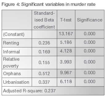
According to this regression model, police stations in more urban areas, with more informal housing, more people renting property, a higher percentage of orphans, and that are relatively poor compared to the rest of the municipality, tend to have a higher murder rate.

Murder rate 10 year average

When looking at the 10 year average murder rate, the influence of a few murders in police precincts with small populations is much lower. Therefore, the analysis could include all the police stations. The variables for population density, unemployment and relative poverty have a significant effect on the 10 year average murder rate per precinct (1 139 included in this analysis).

 

 

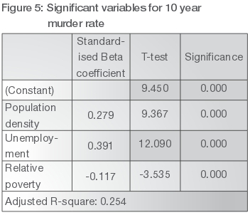
According to this regression model, police stations with a higher population density, higher unemployment rates, and lower relative poverty compared to the rest of the municipality, tend to have a higher average murder rate over 10 years.

 

Discussion on limitations

The use of census data

The estimated population derived using the spatial overlay methodology has certain limitations. Firstly, the census population count may not be accurate. Stats SA corrects for undercounts based on area characteristics, but on a small area level these inaccuracies may not be adequately addressed. Census counting errors can be assumed to differ in different area types. For example, it may be more difficult to count dwellings and households in informal areas, and fieldworkers may not reach all the dwellings in vast rural areas.

Secondly, the households may not be evenly distributed within the small areas, while using straightforward area proportional methodology results in certain households being counted in one precinct while they actually reside in another.

Thirdly, census data are only released every 10 years. The last census was undertaken in 2011, which means that the population distributions may have changed. High mobility and developments in certain areas may result in large shifts in the population per police station that are not accounted for when using the spatial overlay method.

Lastly, using district municipality population growth rates on a local level may also lead to some inaccuracies in the population-per-precinct estimates, as it does not take into account the population changes within the districts. It does, however, allow for a population growth factor to be applied to the police precinct population data when no other estimates for station level population are available.

The use of crime statistics

As noted previously, crime patterns are not evenly distributed. This is also the case in police precincts that differ considerably in size and density. Therefore, precincts have their own crime hotspots but the crime statistics in their current format do not provide disaggregated figures at a street or block level. In addition, under-reporting rates for various crimes may vary across precincts.

Some experts may argue that analysing crime rates at a station level is not going to yield valid results, since crime can be committed during participation in any routine activity that may occur in a different precinct than the one of residence. This is a valid point, as it points to limitations in the format of our current crime statistics. The statistics as they are provided to the public do not provide any information on the place of residence of the perpetrator or the victim. The crime statistics only reflect at which police station the crime was recorded. In the case of murder this is the station under whose jurisdiction the murder occurred, or the victim was found.

Crime research shows that in many urban areas the daytime population is very different to the night-time population. People commute into certain areas to work or look for work during the day, and go home at night. This can skew the reporting at certain stations. Moreover, some crimes are more likely to take place close to home than others.

Due to the large variations in population per precinct, and population densities, murders taking place in precincts with a very low population figure can cause major fluctuations in the murder rate per capita for those precincts. Filtering the smaller precincts (in terms of population) may reduce some of the 'noise' caused by this phenomenon, but it also filters out valuable information from more than a third of the police stations. Other methods of addressing this issue need to be explored. Including other types of violent crime may normalise the population size effect and provide more insight into the effect of socioeconomic factors on violent crime.

 

Discussion on findings and future research

The preliminary statistical analysis above shows a range of associations between murder and precinct-level socioeconomic variables. For instance, the analysis demonstrates that about 25% of murders over a 10-year period can be explained by the variables included in the model.

This and other findings highlight certain considerations for future research. The first is perhaps obvious; that, while basic socioeconomic analysis on its own may indicate significant associations, it will not yield any particularly strong associations with specific socioeconomic variables. This confirms the complexity of the drivers of crimes such as murder.

There may be other crime categories, for instance other violent crimes or property crime, that show stronger associations, but this falls outside the scope of the present study. Previous studies by among others Brown, Breetzke, Demombynes and Ozler would provide some guidance in this regard.²²Applying this methodology to other types of crime may give valuable insights into the socioeconomic factors driving crime, while reducing the effect of some of the limitations of this analysis.

The findings support the notion that more disaggregated crime data at a sub-precinct level, perhaps at an SAL level, could yield more meaningful findings at a neighbourhood level. Essentially, most police station precincts contain different socioeconomic realities within their boundaries.

As highlighted in recent discourses on social disorganisation theory, the drivers of various forms of violent crime and property crime may be diverse, and require multi-level analysis derived from numerous data sources as well as different methodologies.²³At this point in time, limited data are available at a precinct level, which limits the analysis to some very basic socioeconomic indicators.

The analysis in this article should be regarded as exploratory in nature. The methodology employed and findings indicate the complexity of the research required, but also provide a useful springboard for further research. For instance, the independent variables used were developed through this exploratory process, and are by no means exhaustive. Variables such as 'female headed households' are not without controversy, and these debates should be incorporated in future studies.²⁴ Furthermore, future research should include variables from other data sets such as victimisation data, if available, so that more of the issues mentioned in the ecological approach to crime prevention can be incorporated.

 

Conclusions

The data linking methodology used in this study can form the basis for the development of more sophisticated measurements to investigate certain associations between the risk factors identified in the ecological framework. These include the association between crime and poverty, economic deprivation, various indicators of inequality, heterogeneity, mobility, urbanisation, and many other variables identified in recent social ecology discourses. Among these will also be indicators of the impact of social structures and relationships on crime and violence. These indicators include trust in institutions, feelings of belonging or perceptions of social or group integration, and a willingness to show solidarity.²⁵

Precinct-level census information can be used together with other police performance data in the planning of police station-level responses to crime and violence. For example, population figures together with other variables can complement the understanding of the nature of the community serviced by policing structures. In turn it can help inform a rational allocation of resources at police-station level.
 

 

Notes

1 South African Police Service (SAPS), Annual report 2008/09, Pretoria: SAPS, 2009, 10-11.

2 M Shaw, Crime, police and public in transitional societies, Transformation, 49, 2002, 1-24;         [ Links ] GD Breetzke, Modeling violent crime rates: a test of social disorganization in the city of Tshwane, South Africa Journal of Criminal Justice, 38, 2010, 446-52;         [ Links ] G Demombynes and B Ozler, Crime and local inequality in South Africa, World Bank, Policy Research Working Paper 2925, 2002.

3 Shaw & McKay 1942, 1969 cited in L Anselin et al., Spatial analyses of crime, Criminal Justice, 4:2, 2000, 213-262.         [ Links ]

4 Ibid., 217.

5 J Eck et al., Mapping crime: understanding hotspots, Washington DC: National Institute of Justice, 2005, 2.         [ Links ]

6 Anselin et al., Spatial analyses of crime, 217.

7 RJ Sampson and WB Groves, Community structure and crime: testing social disorganization theory, American Journal of Sociology, 94:2, 1989, 774-802,         [ Links ] reprinted in Frances Cullen and Velmer Burton (eds), Contemporary criminological theory, Hampshire: Dartmouth Publishing Co., 1994.         [ Links ]

8 Sampson and Groves, Community structure and crime, 783.

9 Ibid.; BD Warner and P Wilcox Rountree, Local social ties in a community and crime model: questioning the systemic nature of informal social control, Social Problems, 44, 1997, 520-536;         [ Links ] SK Wong, Reciprocal effects of family disruption and crime: a panel study of Canadian municipalities, Western Criminology Review, 8:1, 2007, 48-68.         [ Links ]

10 World Health Organization (WHO), The ecological model, Geneva: WHO, 2012, http://www.who.int/violenceprevention/approach/ecology/en/ (accessed on 15 October 2015).         [ Links ]

11 Ibid.

12 Institute for Security Studies (ISS), Murder and robbery overview of the official statistics: 2014/15, Factsheet, 29 September 2015.

13 Ibid.

14 Eck et al., Mapping crime: understanding hotspots, 2.

15 There is currently no information about population dynamics on a smaller geographical level, which makes it impossible to apply population growth rates on a small area level, Statistics SA, District council projection by sex and age (2002-2004), http://www.statssa.gov.za/publications/P0302/District_Council_projection_by _sex_and_age_(2002-2014).zip (accessed on 15 October 2015).

16 The technical and mathematical description, as well as supplementary selection criteria, falls outside the scope of this article.

17 Sampson and Groves, Community structure and crime, 783.

18 P Blau, Inequality and heterogeneity, New York: Free Press, 1977.         [ Links ]

19 Income measured in October 2011, not indexed.

20 For the purposes of this article, complete tables containing the statistical results for each of these models were left out to ensure ease of interpretation, as the tables with log transformation provide a complex set of results that is difficult to interpret and describe.

21 Collinearity is a condition in multiple regression in which some of the independent variables are highly correlated. Including the smaller precincts in this analysis caused large fluctuations in the murder rate in the small precincts, where one murder in a year would be able to push the murder rate up by 5/100 000.

22 See discussion in Breetzke, Modeling violent crime rates, 446-52.

23 Anselin et al., Spatial analyses of crime, 213-262.

24 M Rogan, Alternative definitions of headship and the 'feminisation' of income poverty in post-apartheid South Africa, The Journal of Development Studies, 49:10, 2013, 1344-1357;         [ Links ] D Budlender, The debate about household headship, Social Dynamics, 29:2, 2003, 48-72.         [ Links ]

25 Organization for Economic Cooperation and Development (OECD), Social cohesion indicators, in Society at a glance: Asia/Pacific 2011, 2012, http://dx.doi.org/10.1787/9789264106154-11-en.; Y Berman and D Phillips, Indicators for social cohesion, paper submitted to the European Network on Indicators of Social Quality of the European Foundation on Social Quality, Amsterdam, June 2004.