Using blinds, day-lighting, and geyser temperature settings to reduce electricity consumption and pricing patterns in energy-efficient buildings

 

 

Godwin Norense Osarumwense Asemota^I; Nelson M. Ijumba^II

^ISenior Member, IEEE
^IISenior Member, IEEE, Fellow, SAIEE

 

 

---

ABSTRACT

Depending on the building architecture, usage, and energy consumption patterns, over US$ 60 billion was expended annually on electric lighting in commercial buildings. Therefore, the paper focuses on the development of energy-efficient buildings that minimize energy consumption through integrated energy-efficient design processes. This can serve as a practical guide to design buildings that can lower the energy requirements and a strategy to reduce energy consumption. In this study, predictive analytics were used to examine how blinds, daylighting, and geyser temperature settings can reduce electricity consumption and pricing patterns. A panel of expert judges was used to validate the 5-point Likert scale residential electricity load management questionnaire used to gather survey data for the statistical analysis in a Windhoek suburb, Namibia. The main goal of this study was to investigate how blinds, day-lighting, and geyser temperature settings can be used to save energy, reduce electricity consumption, and costs for sustainable growth and development. The results from this investigation indicate a perfect Gaussian histogram of 15 electricity price jumps confirming 15 four-way stepwise interaction effects. Optimal 0.5 Quetelet curve index offers average citizen energy efficiency awareness, education, and behavior modification for affordable electricity. Females generally set hotter geyser temperatures and are higher energy consumers. Blinds reduce electricity consumption by 50% in summer, 25% in winter, and day-lighting by 25%. These were the least cost and optimal solutions to the rising electricity consumption and pricing patterns problem. Adopting the findings or the outcomes of this paper could provide more optimal and sustainable energy consumption thereby reducing pressure on the power grid.

Index Terms: Cost-saving, electricity consumption, energy-saving, loss, waste minimization.

---

 

 

I. Introduction

ELECTRICITY supply shortages forced the Southern Africa Development Community (SADC) utilities to implement the demand-side programs [1-2] with load shedding negatively impacted some countries socio-economic development [3]. The Namibian power utility was able to guarantee power till August of 2016 with the occurrence of load shedding. Currently, Namibia generates 40% of its power locally and the remaining 60% from Zambia and Zimbabwe [4]. Namibia's electricity demand doubled in 2012 because of investment in the mining sector, and Eskom supplies over 80% of electricity at significantly increased prices [5]. Liquid fuel constitutes over 63% of total net energy consumption [6] while mining expansion leads to flat load curves [7].

Namibia's electricity price and industrial tariffs are high while South Africa rates are 20 to 25% lower [8]. Reference [9] indicates electricity price increases were to modernize aging infrastructure. The majority of the poor, unemployed, and rural dwelling Namibians [10] cannot afford high electricity prices. Namibia has a harsh weather, dry environment, and acute water shortage problems. The Van Eck dry-cooling power station in Windhoek was built to reduce the water used for cooling [11]. Also, the cooling water needed for the UK's thermal electricity generation fleet is equivalent to that used to cool the Van Eck power plant [12].

Load management (LM) is used to effectively optimize and successfully operate any power utility. Load growth, increasing generation capacity constraints, rising electricity imports, and electricity demand beyond supply capacity in Namibia and Southern African Development Community (SADC), necessitated new generation capacities or LM to supply the shortfall [11]. High energy intensity caused rising electricity tariffs in Namibia [13]. Cost reflective electricity tariffs were anticipated in 2011/2012, and a high supply dependence on South Africa hampers the Namibian electricity supply sector [14].

Blinds systems that comprise curtains, shutters, and shade over windows and doors could reduce inlet heat by 50.0% in summer and 25.0% in heat outlets in winter [11]. Day-lighting is the regulated admission of natural light to reduce electric lighting and save energy. Day-lighting controls provide commercial benefits in the United States (US) because around 75.0% of electricity is consumed in buildings nationwide. Platinum-level rated tubular skylights use 25.0% less energy than conventional lighting fixtures, which incorporates day-lighting to achieve uniform light distribution while limiting electric lighting. Furthermore, day-lighting provides a 24.0% energy reduction in Los Angeles schools and reduces by a third total building energy costs [15].

Total electric energy consumed in commercial buildings is between 35.0% and 50.0%, while between 10.0% and 20.0% of energy used for cooling buildings can be saved by employing day-lighting. Thus, optimization of day-lighting stratagems can reduce total energy costs by a third [16]. Depending on building architecture, usage, and energy consumption patterns, day-lighting could reduce electric lighting between 20.0% and 80.0% [17]. Employing day-lighting at utility peak demand hours can reduce demand charges. Turning off and dimming lights when not needed [1], saves between 10.0% and 20.0% of energy used for cooling a building. This also increases employees' productivity and improves the health of building occupants [18].

Further, above US$60 billion was expended annually for electric lighting that constitutes over 37.0% average commercial buildings' total energy consumption [19]. Also, over 64 billion square feet of commercial buildings floor space was lit by fluorescent systems in which between 30.0% and 50.0% of the spaces can access daylight either by skylights or through windows. Thus, millions of electric lighting fixtures could be turned off for some periods of the day for energy-savings advantages [20].

The objective of the study was to determine how blinds, day-lighting, and geyser temperature settings can be used to save energy, reduce electricity consumption, and costs for sustainable growth and development.

Namibia was the test laboratory. The results, conclusions, and recommendations of the study could be applicable globally. This paper was organized into Introduction, Materials and Methods, Results and Discussion, and Conclusions.

 

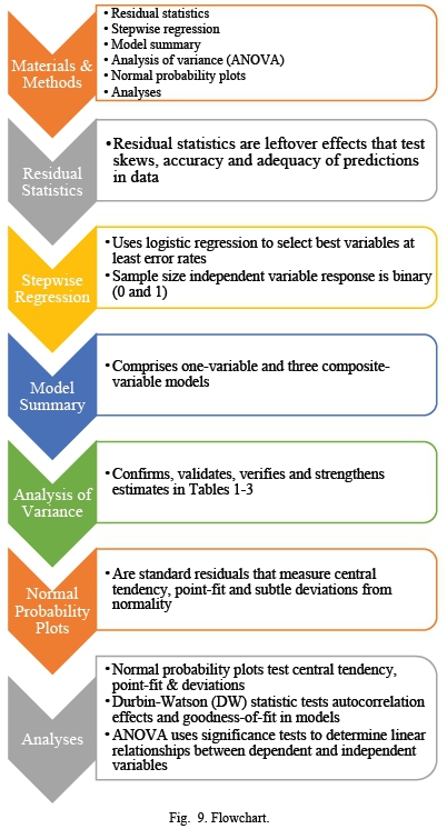
II. Materials and Methods

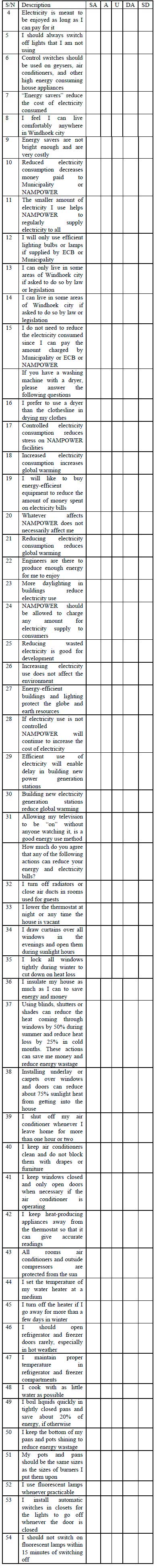
A panel of expert judges was used to validate the 5-point Likert scale residential electricity load management questionnaire used to gather survey data for analysis in Windhoek City, Namibia. Over 300 self-report questionnaires were randomly distributed in Windhoek, Namibia. The 127 returned questionnaires were analyzed using the statistical package for social sciences (SPSS) version 11.5.Also, the 127 sample size sufficiency and adequacy criterion were proved by [21].

The Enter, and Stepwise regression analyses, residuals, analysis of variance (ANOVA), Durbin-Watson statistics, and other methods determined the correctness, model fit, autocorrelation, and overall quality model development [2223]. The study was limited to using blinds, day-lighting, and geyser temperature settings variables to reduce electricity consumption and pricing patterns employing interactional predictive statistics without considering actual electricity consumption measurements of households or other consumers.

The analysis sub-section that applies more complex computational and rational tools to study four tables and eight graphs purely from statistical perspectives can be found in Appendix A. Also, the questionnaire is shown in Appendix B.

2.1. Sample Size Determination

The Cochran formula was used to obtain the sample size, as:

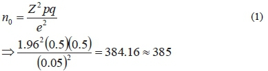
where Z is ± 1.96 ( Z -score values), are probabilities or likely outcomes, e is error (0.05), and study sample size was approximately 385. Also, model diversity decreases with increasing sample size, and a local optimum occurs between 300 and 350 samples [24].

2.2. Residual Statistics

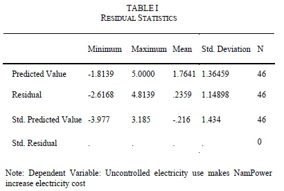
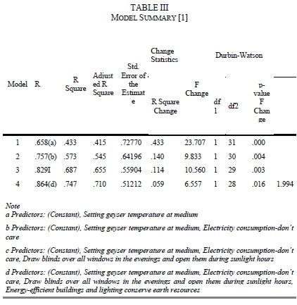
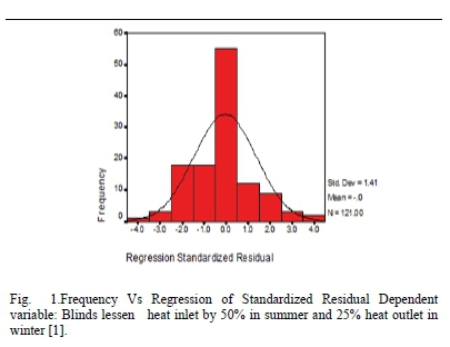
Table 1 indicates the estimates of the disparity between observed and predicted values in regression analyses. The leftover effects test skews, accuracy, and adequacy of statistical predictions in the data. The histogram of standardized residuals is shown in Fig. 1.

2.3. Stepwise Regression

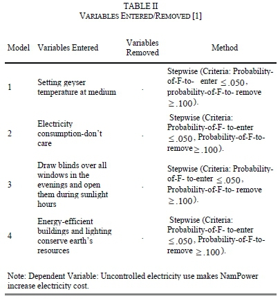
Table 2 was used to present four overall best models. Logistic regression is a stepwise method for selecting the best variables at the lowest error rates. The sample size independent response variable is binary (0 and 1). The four-factor method interprets 15 interdependent interaction effects using (2^k-l), where k is variables number [24].

2.4. Model Summary

Table 3 has one-variable and three composite-variable models. Standard error measures model precision using dependent variable units. The R²change measures advancement in R²upon adding the second evaluator. F change predicts variables addition improvements while the p-value of F change is the alternative hypothesis acceptance probability. Statistical shifts exist between dependent and independent variables [25].

2.5. Analysis of Variance

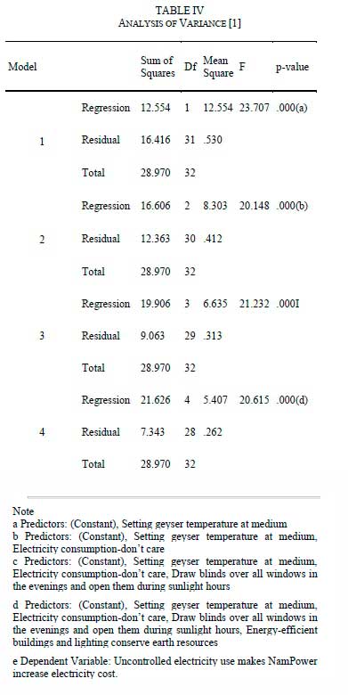
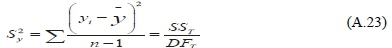
Table 4 is the ANOVA that confirms, validate, verify, and strengthens estimates in Tables 1-3. The sum of squares adds deviations of observations from their mean. The mean square is the variation in the model's measurements. The model is perfect if the model line passes through all the observations [21].

2.6. Normal Probability Plots

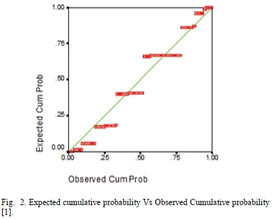
Fig. 2 was used to present the probability-probability plots of standardized residuals. The 0.05 statistical power [26] measures central tendency, point-fit, subtle deviations from normality, and the Gaussian determines the characteristic behavior of increasing electricity prices and consumption patterns.

 

Table 4 was used to present the ANOVA and we determine values of R²and r , for each composite model 1-4.

Model 1: From equation (A.22), the sample square correlation (R₁² ) was 0.4333, and the sample model correlation Ri was

0.6583. The F (1,32) distribution was below 0.0001probability of observing the values over 23.707 and shows strong evidence against the null hypothesis. Thus, ( ) indicates 43.3% variability and 65.8% moderately strong correlation for increasing the price and electricity consumption with hotter geyser temperature settings.

Model 2: From equation (A.22), the sample square correlation (r² ) was 0.5732, and the sample model correlation R²was 0.7571. The F (2,30)distribution was below 0.0001 probability of observing valuesover 20.148 and indicates strong evidence for the alternative hypothesis. Thus, r₂² indicates a 57.3% variability and 75.7% strong correlation for increasing the price and electricity consumption from combined hotter geyser temperature settings and electricity consumption-don't care variables. Thus, model 2 is an improvement over the one variable model.

Model 3: From equation (A.22), the sample square correlation ( ) as 0.6871, and the sample model correlationR3was 0.8289. The F (3,29) distribution was below 0.0001probability of observing values over 21.232 and strong evidence against the null hypothesis. Thus, suggests a 68.7% variability and 82.9% strong correlation at increasing the price and electricity consumption from combined hotter geyser temperature settings, electricity consumption-don't care, and day-lighting variables. There was an improvement over the model having two variables.

Model 4: From equation (A.22), the sample square correlation () was 0.7465, and the sample model correlation r₄was 0.8640. The F (4,28) distribution was below 0.0001probability of observing values over 20.615 and strong evidence for the alternative hypothesis. Thus, indicates 74.6% variability and 86.4% very strong correlation between increasing the price and electricity consumption explained by hotter geyser temperature settings, electricity consumption-don't care, day-lighting and, energy-efficient buildings and lighting conserve earth resources variables. Thus, model 4 was an improvement over all the other three models.

 

III. Results and Discussion

The results are tabulated in Tables 1-4 and Figures 1-8. Figure 9 is the methodology flowchart. Table 1 shows residual statistics and Table 2 indicates stepwise regression results. Table 3 is a model summary for statistics ranging from the coefficient of determination to DW statistic. Table 4 is ANOVA for developed models.

 

 

 

 

 

 

 

 

 

 

 

 

 

 

 

 

 

 

 

 

 

 

 

 

3.1. Histogram of Standardized Residuals

Fig. 1 is a histogram of standardized residuals assessing normality [27]. It cannot detect subtle deviations but tests for normality [28]. The X-axis is Observed Cumulative Probability percentiles in the residuals frequency distribution. The Y-axis is a Standardized Residual (Z-score) for computing the Cumulative Density from the Normal distribution. The normally distributed residuals are on the diagonal of the identity line. Results show 1.41 standard deviations, 0 mean, 0 median, 121 nonmissing samples, and 61^st point of 0 value were the mean and median of the perfect histogram.

3.2. Normal Probability-Probability Plot

Fig. 2 compares the empirical cumulative distribution function (ecdf) of the variable with the defined theoretical cumulative distribution function (tcdf). The proportion of the nonmissing ecdf observations below their heights [29] are sorted according to increasing order. They determine the deviations from normality in the distribution centre, whether Gaussian or not [28]. Linear data distribution point patterns on the P-P plot through the origin are proof that measurements are normally distributed [30]. Therefore, the unit slope in Fig. 2, in square format, is normally distributed [29].

Errors in the Normal P-P plot follow Gaussian normal distributions for parameters [31]. Results in Fig. 2 are nonuniform discrete staircase jump function discontinuities. They are random outcomes in the interval (0, 1) of time distances t. It is a convex set with one minimum point [32-33].

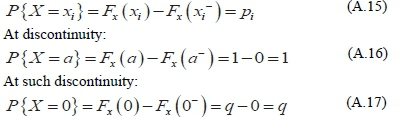
Interchanging axes of F (_x), determine the graph of x_u, the median of x is the smallest number m on the 61^st term in Fig. 1 (m is 0.5 percentile of x).Empirical interpretation of u percentile _x1 is the Quetelet curve [34-35]. This optimization point was n line segments of lengths _x1 , separated vertically in order of increasing lengths. Thus, jump distribution functions occur at 15 points as a countable sequence in Fig. 2.

3.3. Residual Statistics

Table 1 is residual statistics that test remaining variability and the disparity between observed dependent and predicted values in regression analysis. They show the predictions accuracy of models, assumptions, heteroscedasticity, and dispersion in data [36]. Residuals measure the risk premium for operating power systems that affect increasing electricity consumption and pricing patterns [30]. The p-value below 0.0005 suggests perfect model development of statistical significance.

3.4. Variables Entered/Removed Based on Stepwise Regression Analyses

The stepwise method fits models automatically by selecting predictive variables using two significance levels for removal/addition of variable [37]. The probability for adding variables is lower than for removing variables based on t-statistics [38].

Table 2Stepwise criteria have: Probability-of-F-to-enter below 005 (< .050) and Probability-of-F-to-remove variables ( > .100 ) exceeded 0.10. The model variables were removed in one step: set geyser temperature at medium, electricity consumption-don't care, daylighting, and energy-efficient buildings and lighting conserve earth resources.

Setting high geyser temperatures increases electricity consumption and drives electricity prices higher. Not drawing blinds over windows causes higher inlet heat in summer and larger heat outlets in winter. Both factors drive electricity consumption and prices higher for space cooling/heating as shown by the steps/jumps in Fig. 2.

Don't care electricity consumption accentuates higher electricity consumption patterns, higher bills, creates hardship and a vicious spiral for the majority of the population living below the poverty trap [35,39].

However, stepwise analyses significantly strengthen the most economical overall model that contains important variables [40], having minimum predictors [24].

3.5. Model Summary

r measures the relationship between observed and predicted values of the criterion variable. R²tests the criterion variable variance and predictors' goodness-of-fit. Favorable model outcomes could be overestimated. Adjusted R²is the most useful model success indicator [23].

Both R²and standard error ( _S ) measure goodness-of-fit and how the model best fits sample data. _S measures the model precision of the absolute data points spread around the regression line. _S is a rough estimate of 95% prediction interval extending between y_ 2 standard errors of the fitted regression line [25].

The R²values are relative measures of higher variance percentages, while larger R²indicates closely fitted data points. R²is valid for linear models [25], but independent variables collectively explain the variance of the dependent variable. R²measures the relationship strength between the model and the dependent variable on a 0-100% scale. It tests the data scatter points about the fitted regression line [41]. It also contains the precise number of independent variables in regression models [42]. R²change enhances R²by adding a second evaluator. F-test determines the R²change, while significant F -change suggests that the added variables remarkably enhanced the prediction [43]. The limitations of R²include prescription bias when the linear model was underspecified. Further, significant independent variables, polynomials, or interaction terms are present [41].

A. 3.5.1. Model 1 Setting Geyser Temperatures at Medium

The 65.8% correlation and 43.3% variance accounted for in model 1, occurred between setting geyser temperatures at medium against increasing electricity consumption and pricing patterns. Overall model fit improved 41.5%, 0.73% standard distance between observation and regression lines, 95% data points are between the regression line and / 1.5% of geyser temperature settings. Hence, Model 1 is statistically significant ( F_m= 23.707 ; p ! 0.0005)^.

3.5.2. Model 2 Combined Effects of Geyser Temperature Settings and Electricity Consumption-Don't Care

Over 75.7% correlation and above 57.3% variance were allowed in Model 2. Overall model fit improved 54.5%, 0.64% standard distance between observation and regression lines, 95% data points of model lie between the regression line and +/_- 1.3% of combined effects of geyser temperature settings and electricity consumption-don't care. Model 2 improved 14.0% by adding a second predictor. It was statistically significant ()^.

3.5.3. Model 3 Combined Effects of Geyser Temperature Settings, Electricity Consumption-Don't Care and Day- lighting

Above 82.9% correlation and over 68.7% variance were allowed in Model 3. About 65.5% overall model fit sufficiency, 0.56% standard distance between observation and regression lines, 95% model precision of data points lie between the regression line and /1.12% of geyser

temperature settings, electricity consumption-don't care, and day-lighting. An incremental 11.4% model improvement was achieved by adding the third predictor. Model 3 was statistically significant )^.

3.5.4. Model 4 Combined Effects of Geyser Temperature Settings, Electricity Consumption-Don't Care, Day-lighting, and Energy-Efficient Buildings and Lighting Conserve Earth Resources

About 86.4% correlation and over 74.7% variance were allowed in Model 4. Above all, the 71.0% overall model goodness-of-fit, 0.51% standard distance of observation and regression lines, occurred while 95% of the model data precision points lie between the regression line and / 1.0% of the geyser temperature settings; electricity consumption-don't care; day-lighting and energy-efficient buildings and lighting conserve earth resources. Model 4 achieved a 5.9% incremental improvement by adding four predictors and was statistically significant ()^.

3.6. The Durbin-Watson Statistic

Overall, the 71.0% model goodness-of-fit mirrors increasing electricity consumption and pricing patterns. Therefore, the researchers accept the null hypothesis of the DW statistic because the effective DW (2.006) was higher than the upper limit of the DW statistics (d_v= 173). We also conclude that there were no autocorrelation effects in the model. This was so because the determined DW (1.994) was close to the ideal DW statistic (Since 4 -1.994 = 2.006 2.0 ). Therefore, errors in the model were uncorrelated, without autocorrelation effects, and without violating the independent errors assumption of the Durbin-Watson statistic [44-45]. The two (2) DW statistics suggests a very excellent model and also strengthens the significance, quality, and adequacy of this and the other four (4) developed models, in this paper.

3.7. Multivariate Interaction Effects

Interaction effects occur whenever one variable effect depends on another and affect statistical design outcomes. They show how a third variable influences links between dependent and independent variables [46]. The p-values are the statistical significance of fitted interaction plots. Several lines indicate the values of the second independent variable [46], while the parallel lines show no interaction effects. Different slopes suggest interaction effects. The cross-lines on the graph indicate that the interaction effects have significant p-values and so, the main effects are interpreted [46].

Logistic regression models use stepwise to select the best model, give the lowest error rates, broad usage, and sample size independence. The model diversity evaluates the model quality for reproducibility and each interaction effect indicates the compound power index [24].

3.7.1. Model 1a Setting Geyser Temperatures at Medium-Main Interaction Effect (A)

Model 1a: This factor is highly significant in electricity load management because the specific heat capacity of water is high, and setting geyser temperature at medium reduces energy wastage [1,47].

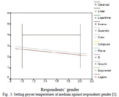
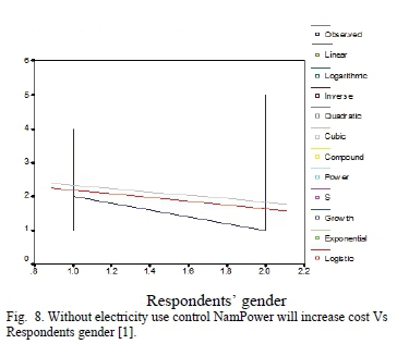
Further, the Y-axes for Figs. 3-8 are response figures on a 5-point Likert scale. The 9-point Likert scale on Y-axis for Fig. 5 arose because 9 was used to represent missing responses on the questionnaire (attached). The X-axes for Figs. 3-8 were supposed to have 1 and 2 only because each represents male and female. The fractional or decimal values on X-axis arose because of the limitations and drawing errors of automatically using the preset scaling graph algorithms in SPSS software. Therefore, decimal figures on the X-axes for Figs. 3-8 should be ignored as machine errors because males and females are binary and there are no fractions in human beings.

Fig. 3 suggests an H-pole with parallel decreasing logistic and cubic regression cross-lines. The graph shows females set higher geyser temperatures, cause higher electricity consumption and higher prices. The growth regression cross-line plateaued [46] at level four (4), which means hotter geyser temperatures settings by both genders lead to higher electricity consumption, higher electricity prices, and higher utility penalty payments. However, the vertical parallel lines on points 1 and 2 of the X-axis indicate there were no interaction effects [24] between the gender and everyone (male or female) was at liberty to set hotter geyser temperatures.

3.7.2. Model 1b Electricity Consumption-Don't Care-Main Interaction Effect (B)

Model 1b: works directly into the economic objectives of utility and could negatively impact electricity supply efficiency and usage, electricity bills, and loss reduction. This behavioral attitude in electricity consumption stresses utility facilities, provides a strong economic basis for electricity price increases, which supports utility production inefficiencies and could jeopardize the public good, in terms of energy efficiency [1].

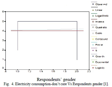
Fig. 4 indicates an eta-shaped or table-like plateau of growth regression interaction cross-lines. It has high and slowly rising logistic and cubic regression gradients by gender. The graph shows the highest rates of electricity consumption and penalty payments by both genders. The interaction cross-lines of logistic and cubic regressions, as well as the entitled electricity consumers groups, were gender independent [46]. This was so because the vertical parallel lines on points 1 and 2 on the X-axis (respondents' gender) indicate no interaction effects across gender in electricity consumption. Further, the figures on Y-Axis indicate (1-strongly agree, 2-agree, 3-not sure, 4-disagree, and 5-strongly disagree) the strength of respondents agreeing with the propositions on the questionnaire.

3.7.3. Model 1c Day-lighting-Main Interaction Effect (C)

Model 1c conserves heat, lowers energy or electricity consumption, and electricity are bills paid for home heating by natural convection. These reduce wasted energy, greenhouse gases (GHG) emissions, fuel burnt for electricity production, and avoided production [1,47], defer high-cost power plants, transmission, and distribution network systems [30].

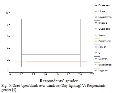
Fig. 5 suggests indecision in using day-lighting to reduce electricity consumption as shown by the horizontal crossbar of H-pole growth regression cross-lines. Day-lighting practice hovers between strongly agree and agree for logistic and cubic regression interaction patterns. Therefore, day-lighting indicates the optimal solutions to reducing electricity consumption and pricing patterns problem by gender, because there were no gender interactions in using it to reduce consumption and costs. Additionally, [15] indicates day-lighting reduces electricity consumption by 25%.

Therefore, day-lighting is one of the best strategies for keeping electricity consumption and price increases to the barest minimum. It could be pivotal in any electricity load management model for securing optimal and sustainable production, transmission, distribution, and utilization of electrical power, globally.

3.7.4. Model Id Energy-Efficient Buildings and Lighting Conserve Earth Resources-Main Interaction Effect (D)

Model 1d: directly relates the stress on utility facilities with power consumed always. Electricity consumers' gender, economic power, and age determine preferences in an electrical appliance used and times of use for households, lighting, or electric motors in commerce and industry. The quantity and cost of electricity used depend on the application [1], which affects electricity pricing [30] and stresses placed on utility facilities [47].

Electricity production technologies use coal, natural gas, diesel, the nuclear, hydro, wind, and solar while increasing electricity consumption worldwide increases global warming. Utilities unable to cope with overloads lead to power systems failures, instability, unreliable performance, and nonconformance with regulatory requirements [1].

Fig. 6 suggests wheel and axle-type interaction plots for logistic, cubic, and growth regressions. Male electricity consumers prefer energy-efficient buildings and lighting. Although the spread is gender independent, females have a larger scatter. Electricity consumption patterns were equal at mid-points for cubic and growth regressions (1.5) and logistic and growth regressions were close to 1.1. Thus, males were more favorably disposed to energy-efficient building and lighting principles and practices.

3.7.5. Using Blinds Reduce Heat Inlet through Windows by 50% in Summer and Heat Outlet by 25% in the Winter-Main Interaction Effect

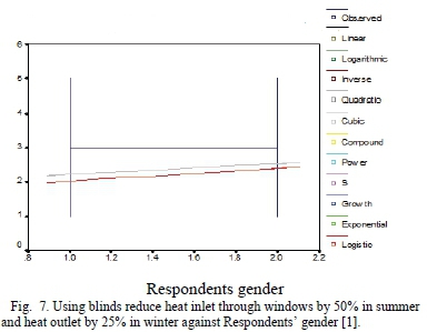
Fig. 7 is an H-pole growth regression with almost parallel logistic and cubic interaction cross-lines. Blinds reduce inlet heat through windows by 50% in summer while not running air conditioners or other cooling devices. It reduces heat exchanges between warmer inside ambience with much colder outside temperatures by 25% in winter, while heaters are on [1]. This reduces electricity consumption for room and space heating/cooling. Electricity prices were stable, even during heavy, persistent, and universal electricity consumption. The plateau [46] between the H-pole cross-line indicates virtually no increases in electricity consumption or prices and no interaction effects across gender.

However, both the logistic and cubic interaction cross-lines show increasing electricity consumption and pricing patterns if those using blinds were male.

3.7.6. Uncontrolled Electricity Use Makes NamPower Increase Electricity cost-Main Interaction Effect

Fig. 8 is a J-shaped interaction plot of growth, logistic and cubic regression cross-lines. The parallel lines [46] indicate no interaction effects across gender that controls rising electricity consumption and cost patterns, but high electricity consumption and pricing patterns are prevalent if consumers are female. However, the rate of increase is much higher for the growth regression line than either the logistic or cubic regression interaction cross-lines. Thus, costs are managed by reducing consumption, peak load management, peer comparison, and energy efficiency identification projects, utility invoice management that optimize facility, and involvement in rate-making processes [48].

3.7.7. One-Way Effects for each of the Four (4) Main Interaction Effects- a bc d

The model of each main effect predicts how their combined effects encourage rising electricity consumption and pricing patterns. Adjusted R²value indicates the quality of the model and accounts for over 41.5% variance. Thus, rising prices and electricity consumption depend on geyser temperature settings (A), electricity consumption-don't care (B), Day-lighting (C), and energy-efficient buildings and lighting conserve earth resources ( D) ·

3.7.8. Two-WayEffects(a,B,axb)

Model 2 is the interaction and predictive relationships of setting high geyser temperatures and electricity consumption-don't care. Adjusted R²value accounts for over 54.5% variance in total overall model development. The three major

relationships were: (a) main effect (A), (b) main effect (B), and (c) single two-way interaction of items A and B ( A χ B) .The additional 13% variance was a combination of items A and B, each acting alone and in concert (A χ B) [1,22-23]. To

avoid repetition, the single two-way interaction (A χ B)is discussed. Hence, rising price and electricity consumption patterns depend on the combined effects of hotter geyser temperature settings and electricity consumption-don't care (A χ B).

3.7.9. Three-Way Effects of Combining the First Three (3) Main Effects (Seven Model Effects in All)

Model 3 is the interaction and predictive relationships among three variables: (i) setting high geyser temperatures (A), (ii)

electricity consumption-don't care ( B), and (iii) day-lighting (C )^.

There were seven models: (a) main effect (A), (b) main effect (B), (c) main effect (C), (d) two-way effect (A χ B), (e) two-way effect (AxC), (f two-way effect (β_χc), and (g) single three-way effect ( a χ B χ C).

Adjusted R²value accounts for over 65.5% variance in total overall model development. This suggests an additional 11.0% variance above the model with only two interacting predictors [1].

To avoid repetition, only the three two-way effects and one three-way effect are discussed. Therefore, rising price and electricity consumption patterns depend on the combined effects of high geyser temperature settings and electricity consumption-don't care (A χ B), high geyser temperature settings, and day-lighting (Α_χC), electricity consumption-don't care and day-lighting ( β _χc ) and high geyser temperature settings, electricity consumption-don't care and day-lighting ( Αχ B χ C )^.

3.7.10. Four-Way Effects Combine the Four (4) Models Selected by the Stepwise Regression (15 Models)

The four-way effects of model 4 indicate relationships between four predictors: (i) setting high geyser temperatures (A) ; (ii) electricity consumption-don't care (B) ; (iii) day-lighting (C ), and (iv) energy-efficient buildings and lighting conserve earth resources ( D).

The fifteen models were: (a) main effect (A), (b) main effect (B ), (c) main effect (C), (d) main effect (D), (e) two-way effect (A χ B), (f two-way effect (Α_χ C), (g) two-way effect (a _χ D), (h) two-way effect (β _χc) two-way effect(g _χ d), (j) two-way effect(c _χ D), (k) three-way effect ( A χ B χ D ) ; (l) three-way effect ( Αχ B xC ), (m) three-way effect (b χ C χ D), (n) three-way effect (a χ C χ D), and one four-way effect (Αχ B χ Cχ D).

The final Adjusted R²value accounts for over 71.0% variance in the total overall model developed. The result shows an additional 5.5% variance contribution over the model with three interacting predictors. The trend indicates that additional variance contributions from higher-order interacting predictor variables, continuously improved upon the quality of model fit in the study (71.0% model fit with 4 predictors). To avoid repetition we discuss only the combined effects.

Thus, rising price and electricity consumption patterns depend on: high geyser temperature settings and electricity consumption-don't care ( A χ B), high geyser temperature settings and day-lighting(Α_χC), high geyser temperature settings and energy-efficient buildings and lighting conserve earth resources ( Α_χ D), electricity consumption-don't care and day-lighting (β _χc), electricity consumption-don't care and energy-efficient buildings and lighting conserve earth resources ( β _x d), day-lighting with energy-efficient buildings and lighting conserve earth resources (c _x D), high geyser temperature settings, electricity consumption-don't care and day-lighting (a_xb_xc), high geyser temperature settings, electricity consumption-don't care and energy-efficient buildings and lighting conserve earth resources (a _x b _x d), high geyser temperature settings, day-lighting and energy-efficient buildings and lighting conserve earth resources(a_xc_xd), electricity consumption-don't care, day-lighting with energy-efficient buildings and lighting conserve earth resources (β _x c _x D), and high geyser temperature settings, electricity consumption-don't care, day-lighting with energy-efficient buildings and lighting conserve earth resources ( a x b x c x d) ·

Nevertheless, the 15 jump discontinuities in Fig. 2 corroborate the 15 four-way effects developed by the stepwise regression in Table 3. The same trend of reinforcements and validations are visible from the parameter estimates in Tables 1, 3, and 4, which have all worked in tandem to strengthen the claims of very good model development having the requisite accuracy, precision, and reliability in this paper.

ANOVA splits observed variance for significance and tests whether linear relationships exist between dependent and independent variables [49]. The error sum of residuals is a portion of total variability not explained by the model and nonlinear portions of the dependent variable [22],[23],[45],[49]. Although the F-test does not indicate which parameters is not zero, only that at least one of them is linearly related to the response variable. Further, the square root of R²is the multiple association coefficient r between observations yi and fitted values [50].

The distribution F(1,32)has below 0.0001 probability of observing a value over 23.707 and strong evidence for the alternative hypothesis. Thus, indicates 43.3% variability and 65.8% moderately strong correlation explained by increasing price and electricity consumption patterns for high geyser temperature settings. Also, the distribution F₍₂₃₀₎ has below 0.0001 probability of observing a value over 20.148 and strong proof for the alternative hypothesis. Thus, r₂² suggests 57.3% variability and 75.7% strong correlation explained by increasing price and electricity consumption patterns for the combined high geyser temperature settings and electricity consumption-don't care variables. This was 14.0% better than the one variable linear model.

The distribution F(₃₂₉) has below 0.0001 probability of observing a value over 21.232and strong indication against the null hypothesis. Thus r₃² implies 68.7% variability and 82.9% strong correlation explained by rising price and electricity consumption patterns for the combined high geyser temperature settings, electricity consumption-don't care, and day-lighting variables. There was an 11.0% enhanced performance over the two variables model.

The distribution F _(4,28) has below0.0001 probability of observing a value exceeding 20.615 and strong evidence against the null hypothesis. Thus, stipulates over 74.6% variability and 86.4% very strong correlation explained by increasing price and electricity consumption patterns for combined high geyser temperature settings, electricity consumption-don't care, day-lighting with energy-efficient buildings and lighting conserve earth resources variables.

There was an extra 5.9% refinement over all the other models and especially that having only three variables.

 

IV. Conclusions

Using blinds, shutters, or shades significantly reduced inlet heat through windows by 50.0% in summer and heat outlet by 25.0% during winter, while day-lighting reduced electricity consumption by 25.0% as electricity prices were stable, even during heavy, persistent, and widespread electricity consumption.

Both electricity price jump discontinuities and stepwise regression four-factor interaction analyses were 15 each, and the 0.5 Quetelet curve index at median percentile was the optimal solution to the empirical electricity consumption and net pricing distribution patterns problem. Furthermore, the Quetelet index is used to create awareness, education, and behavior modification especially among the average citizens on energy efficiency for affordable, reliable, and sustainable supply.

Logistic and cubic interaction cross-lines show males prefer using blinds over windows than females. Blinds and day-lighting were the least cost and optimal strategies for curtailing electricity consumption and latching price increases. Therefore, blinds and day-lighting could lead to optimal and more sustainable production, transmission, distribution, and utilization of electrical power, worldwide. Future research should consider actual electricity consumption measurements by electrical appliances category to ascertain quantifiable energy savings. Consequently, actual electricity consumption measurements of appliances in households and other consumers could be used to better understand the cause-effect relationships and to determine specific energy savings from particular and specialized consumer categories.

 

Acknowledgment

This is an extended and updated version of an unpublished paper (not published in IEEExplore), originally accepted for the IEEE International Conference on Industrial Technology (IEEE ICIT 2013) held in Cape Town, South Africa between 25 and 27 February 2013.

 

References

[1] S. Bimenyimana, A. Ishimwe, G. N. O. Asemota, C. M. Kemunto, and L. Li, "Web-based design and implementation of smart home appliances control system," in ICRET, Kuala Lumpur, Malaysia. IOP Conf. Series: Earth andEnv. Sci., vol. 168, pp. 1-9, 2018, 10.1088/1755-1315/168/1/012017        [ Links ]

[2] P. Warren, "Demand-side policy: Global evidence base and implementation patterns," Energy and Env., pp. 1-26, 2018, 10.1177/0958305X18758486

[3] P. I. Shilamba, "Update on the current power supply and progress made on NamPower projects and initiatives to ensure security of supply in Namibia," Media Briefing, Windhoek, Namibia. 13 April, 2015.

[4] Anon., "No power cuts expected in Namibia-Energy Minister," New Era Newspaper, Windhoek, Namibia. 24 Mar. 2016. [Online]. Available: https://www.newera.com.na/2016/03/24/power-cuts-expected-namibia-energy-minister/, Accessed on: Mar. 29, 2017

[5] W. Isaaks. Energy situation in Namibia. Presented at AEF2013 Africa Energy Forum, Barcelona, Spain. [Online]. Available: www.energynet.co.uk/system/files/Private 23, Accessed on: Mar. 29, 2017

[6] V. Manuel, "Energy demand and forecasting in Namibia: Energy for economic development." Office of the President, National Planning Commission, Windhoek, Namibia. 2013.

[7] P. Simshauser and D. Downer, 2012. "Dynamic pricing and the peak electricity load problem," AustralianEcon. Rev., vol. 45, no. 3, pp. 305-324, 2012, 10.1111/j.1467-8462.2012.00687.x.         [ Links ]

[8] E. Brandt, "Namibia's high electricity price," New Era Newspaper, Windhoek, Namibia. 14 Nov. 2014. [Online]. Available: http://allafrica.com/stories/201411140794.html, Accessed on: Mar. 29, 2017

[9] P. Warren, "Demand-side policy: Global evidence base and implementation patterns," Energy and Env., pp. 1-26, 2018, 10.1177/0958305X18758486

[10] CIA World Factbook, "Namibia Economy 2018," [Online]. Available: https://theodora.com/wfbcurrent/namibia/namibia-economy.html

[11] G. N. O. Asemota Electricity Use in Namibia. Bloomington, IN, USA: iUniverse, 2013.

[12] D. Murrant, A. Quinn, L. Chapman, and C. Heaton, "Water use of the K thermal electricity generation fleet by 2050: Part 2 quantifying the problem," Energy Policy, vol. 108, pp. 859-874, 2017, 10.1016/j.enpol.2017.03.047        [ Links ]

[13] Electricity Control Board, "2005 Electricity Control Board Annual Report." ECB, Windhoek, Namibia, Annual Report, 2006.

[14] D. von Oertzen, "Namibia's Electricity Supply." VO Consulting,. Swakopmund, Namibia. 2009. [Online]. Available: https://www.voconsulting.net/pdf/Namibia's%20Electricity%20Supply%20-%20VO%20CONSULTING.pdf

[15] Solatube,"Daylighting Facts & Figures," [Online]. Available: 150516 Daylighting Facts & Figures-plain.pdf

[16] G. Ander, "Day-lighting: Whole building design guide," 2011. [Online]. Available: http://www.wbdg.org/resources/daylighting.php

[17] N. Stauffner, "Daylight Device Lightens Electricity Cost," MIT News, 2007. [Online]. Available: http://newsoffice.mit.edu//2007/techtalk51-26.pdf

[18] D. Kozlowski, "Using daylighting to save on energy costs," FacilitiesNet, 2006. [Online]. Available: http://www.facilitiesnet.com/energyefficiency/article/Harnessing-Daylight-For-Energy-Savings-Facilities-Management-EnergyEfficiency-Feature-4267#

[19] T. Mocherniak, "Lighting technologies produce energy savings," Energy and Power Mgt., 2006. [Online]. Available: www.highbeam.com/doc/1G1-146346289.html

[20] R. P. Leslie, R. Raghavan, O. Howlett, and C. Eaton, "The potential of simplified concepts for daylight harvesting," Lighting Research and Technology, 2005. [Online]. Available: http://www.lrc.rpi.edu/programs/daylighting/pdf/simplifiedConcepts.pdf

[21] G. N. O. Asemota, "Communality performance assessment of electricity load management model for Namibia," Presented at 2^nd IEEE-AIMS Int. Conf., Madrid, Spain, pp. 252-257, 2014, 10.1109/AIMS.2014.20

[22] J. J. Foster, Data analysis using SPSS for Windows: a beginner's guide. 2nd ed., London, UK: Sage Publication, 1998.

[23] N. Brace, R. Kemp, and R. Snelgar, SPSS for Psychologists: a guide to data analysis using SPSS for Windows. New Jersey, NJ, USA: Lawrence Erlbaum Associates, 2000.

[24] T. Heckmann, K. Gegg, A. Gegg, and M. Becht, "Sample size matters: investigating the effect of sample size on a logistic regression susceptibility model for debris flows," Nat. Hazards Earth Syst. Sc., vol.14, pp. 259-278, 2014, 10.5194/nhess-14-259-2014.         [ Links ]

[25] J. Frost, "Standard error of the regression vs r-squared,". 2017a. [Online]. Available: Statisticsbyjim.com/regression/standard-error-regression-vs-r-squared/, Accessed on: Jan. 23, 2019

[26] G. N. O. Asemota, "Evidence-based wind-felled recovery of plantains," Afr. J. Plant Sci. Biotech., vol. 4, no. 1, pp. 84-89, 2010.         [ Links ]

[27] M. Beasley, "BST 622 regression assumptions-graphs," [Online]. Available:www.soph.uab.edu/statgenetics/People/MBeasley/Courses/BST622RegressionAssumptions-Graphs.pdf, Accessed on: Mar. 29, 2017

[28] K. Grace-Martin, "Anatomy of a normal probability plot: The analysis factor," [Online]. Available: http://www.theanalysisfactor.com/anatomy-of-a-normal-probability-plot/

[29] SAS Institute Inc, "Construction and interpretation of P-P plots," 1999. [Online]. Available: https://v8doc.sas.com/sashtml/qc/chap8/sect8.htm, Accessed on: Mar. 29, 2017

[30] G. N. O. Asemota, "A prediction model of future electricity pricing in Namibia," Adv. Mat. Res., vol. 824, pp. 93-99, 2013, 10.4028/www.scientific.net/AMR.824.93.         [ Links ]

[31] D. George and E. A. Huerta, "Deep neural networks to enable real-time Multimessenger Astrophysics," ArXiv:1701.00008v2 [astro-ph.IM], 4 Jan. 2017.

[32] G. N. O. Asemota, "On a class of computable convex functions," Can. J. Pure and Appl. Sci., vol. 3, no. 3, pp. 959-965, 2009.         [ Links ]

[33] G. N. O. Asemota, "Optimal two-way conductor design using computable convex functions approach," Adv. Mat. Res., vol. 367, pp. 75-81,2012, 10:4028/www.scientific.net/AMR.367.75        [ Links ]

[34] A. Papoulis and S. U. Pillai, Probability, random variables and stochastic processes. 4th ed., New Delhi, India: Tata McGraw-Hill, 2008.

[35] G. Jahoda, "Quetelet and the emergence of the behavioral sciences," SpringerPlus, vol. 4, pp. 473, 2015. [Online]. Available: https://www.ncbi.nlm.nih.gov/pmc/articles/PMC4559562/, Accessed on: Jul. 30, 2018        [ Links ]

[36] J. J. Taylor, "Confusing stats terms explained: residual," 2011. [Online]. Available: www.statsmakemecry.com/smmctheblog/confusing-stats-terms-explained-residual.html, Accessed on: Jan. 5, 2019

[37] NCSS statistical software, "Stepwise regression: Chapter 311," [Online]. Available: https://ncss-wpengine.netdnassl.com/wp-content/themes/ncss/pdf?procedures/NCSS/stepwiseRegression.pdf, Accessed on: Jan. 5, 2019

[38] R. Nau, "Stepwise regression and all-possible-regressions-Duke people," 2014. [Online]. Available: https://people.duke.edu/~rnau/regstep.htm, Accessed on: Jan. 5, 2019

[39] CIA World FactBook, "Namibia Economy 2018," [Online]. Available: https://theodora.com/wfbcurrent/namibia/namibia-economy.html, Accessed on: Jul. 30, 2018

[40] E. Marshall, "The statistics tutor's quick guide to commonly used statistical tests," [Online]. Available: www.statstutor.ac.uk/resources/uploaded/tutorquickguidetostatistics.pdf, Accessed on: Jan. 9, 2019

[41] J. Frost, "How to interpret r-squared in regression analysis," 2018. [Online]. Available: Statisticsbyjim.com/regression/interpret-r-squared-regression/, Accessed on: Jan. 23, 2019

[42] J. Frost, "How to interpret adjusted -r-squared and predicted r-squared in regression analysis," 2017b. [Online]. Available: Statisticsbyjim.com/interpret-adjusted-r-squared-predicted-r-squared-regression/, Accessed on: Jan. 19, 2019

[43] J. T. Newsom, "Lecture 20: more on multiple regression," 2007. [Online]. Available: Web.pdx.edu/~newsomj/PR551/lecture20.htm, Accessed on: Jan. 29, 2019

[44] M. R. Braun, H. Altan, and S. B. M. Beck, "Using regression analysis to predict the future energy consumption of a supermarket in the UK," Appl. Energy, vol. 130, pp. 305-313, 2014, 10.1016/j.apenergy.2014.05.062        [ Links ]

[45] G. N. O. Asemota, "Multivariate parsimony model of electricity load management," WSEAS-10^th Energy and Env. Int. Conf., Budapest, Hungary, 2015, pp. 77-86.

[46] J. Frost, "Understanding interaction effects in statistics," 2017c. [Online]. Available: Statisticsbyjim.com/regression/interaction-effects/, Accessed on: Jan. 30, 2019

[47] P. Jones, How to cut heating and cooling Costs: save money and energy in your home. New York, NY, USA: Butterick Publishing, 1979.

[48] Energywatch, "Why your electricity bills increase despite low power pricing," 2019. [Online]. Available: https://energywatch-inc.com/electricity-bills-increase-despite-low-power-pricing/, Accessed on: Feb. 8, 2019

[49] Weibull.com, "Reliability hot wire: Analysis of variance," [Online]. Available: https://www.weibull.com/hotwire/issue95/relbasics95.htm, Accessed on: Feb. 11, 2019

[50] M. Lacey, "ANOVA for regression," [Online]. Available: www.stat.yale.edu/Courses/1997-98/101/anovareg.htm, Accessed on: Feb. 11, 2019

[51] F. B. Hildebrand, Advanced calculus for application. 2nd ed., New Delhi, India: Prentice-Hall of India Private Limited, 1977.

[52] J. Waldvogel, "Circuits in power electronics," in Solving problems in scientific computing using Maple andMATLAB, 4th ed., W. Gander and J. Hrebicek, Eds. Berlin, Germany: Springer, 2004, pp. 314.

[53] J. Netter, M. H. Kutner, C. J. Nachtsheim, and W. Wasserman, Applied linear regression. 3rd ed., USA: Irwin, 1996.

[54] A. H. Kvanli, S. C. Guynes, and R. J. Pavur, Introduction to business statistics: A computer integrated approach. 4th ed., St. Paul, Minneapolis, MN, USA: West Publishing Company, 2002.

 

 

 

Godwin Norense Osarumwense Asemota (M'2004-SM'2013), became a Member (M) of IEEE in 2004 and a Senior Member (SM) in 2013. He holds a B.S. in physics, post graduate diploma in electrical and electronics engineering, M.S. in electronic and electrical engineering, MBA in finance and banking, and Ph.D. in electrical engineering. He researches in electricity load management, power systems engineering, convex functions mathematics, plantains biology, finance and banking, renewable energy systems, power systems control, and optimization.
He taught high voltage engineering, power systems engineering, power plants engineering, and research methodology at the Kigali Institute of Science and Technology (Now College of Science and Technology, University of Rwanda, Kigali, Rwanda). He is currently at the African Centre of Excellence in Energy for Sustainable Development, University of Rwanda, Kigali, Rwanda and Morayo College, Nairobi, Kenya.
Dr. Asemota has published over seventy journal articles and conference papers, Electricity Use in Namibia, iUniverse, 2013, and Application of Modern Load Flow Techniques to Electric Power Systems, Lambert, 2010.

 

 

Professor Nelson Ijumba is the International Research and Innovation Programme Manager, based in the Africa Hub of Coventry University. He is Emeritus Professor of Electrical Engineering at the University of Rwanda, based in the African Centre of Excellence in Energy for Sustainable Development (ACEESD), and also an Honorary Professor of Electrical Engineering, at the University of KwaZulu Natal, South Africa. He has over 40 years of experience in teaching, research, consulting and academic leadership.
His research and consultancy services are in green energy, renewable energy resources exploitation, energy efficiency, electrical power systems, high voltage technology, innovation, higher education management and engineering education. Prof Ijumba is passionate about the impact of technologies on sustainable development and translation of research outputs into socially relevant innovative products. Professor Ijumba graduated from the University of Dar es Salaam (Tanzania), and obtained his Master's and Doctoral degrees from the Universities of Salford and Strathclyde (United Kingdom), respectively. He is a Fellow of the Southern African Institution of Electrical Engineers, a Senior Member of the Institute of Electrical and Electronics Engineers, a Member of the Institution of Engineering and Technology. Professor Ijumba is a Member of the Academy of Sciences of South Africa and a Fellow of the South African Academy of Engineering.
He is a registered Professional Engineer with the Engineering Council of South Africa; the Engineering Registration Board of Tanzania and a Chartered Engineer of the United Kingdom Engineering Council. He has published widely in indexed journals and made numerous presentations at international and local conferences.
This paper was submitted on 24 October 2020 for review. This work was funded by the African Centre of Excellence in Energy for Sustainable Development, University of Rwanda, Kigali, Rwanda.
GNO Asemota is with Morayo College, Nairobi, Kenya and African Centre of Excellence in Energy for Sustainable Development, University of Rwanda, Kigali, Rwanda (e-mail: asemotaegno@gmail.com).
NM Ijumba is with the School of Engineering, University of KwaZulu-Natal, Durban, South Africa and African Centre of Excellence in Energy for Sustainable Development, University of Rwanda, Kigali, Rwanda (e-mail: n.ijumba@ur.ac.rw).

 

 

Appendix

I. Appendix A

A.1. Analyses This section contains the analyses of the study.

A.1.1. Normal probability-probability plot

Fig. 2 is a Normal P-P plot that compares the variable empirical cumulative distribution function (ecdf) with the theoretical cumulative distribution function (tcdf) F(.). The ecdf Fn(x) is the nonmissing observation proportion equivalent to x, because . Furthermore, the n nonmissing values follow an increasing order [29] :

The i^thordered value X® on the P-P plot in the X-coordinate is , and in the Y-coordinate is [i/n].

Errors in the Normal P-P plot follow Gaussian normal distributions for parameters [27],[31].

Fig. 2 was used to present the results of discrete nonuniform staircase jump functions. They lie along with electricity consumption against the net pricing distribution curve. Electricity switching and consumption patterns are random intervals (0, 1). Their time distances, t occur between 0 and 1. The probability t is between ti and t2 [34] :

The random variable X is

The variable has double meanings: Experimentation outcome and also, corresponding value x(t) of random variable X. We show the ramp distribution function, F(x) of X [34]: If χ > 1, then _x (_t) < _χfor every outcome:

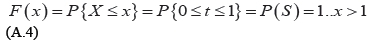
If 0 < x < ι, then X (t ) £ x for every t in interval ( 0, χ )

Thus:

F(x) = P{X £ x} = P{0 £ t £ x} = x...0 £ x £ 1 ^(A.5) If χ < 0 , then {χ < _x} is the impossible event because X (t) > 0 for every t. Whence,

Established as, required.

Percentile η of the random variable X is the smallest number Xu because [34]:

Hence, Xu is the inverse of the function _u= f (χ), ininterval ο < _u < I, on the X-axis. We interchange the axes of F(x) to determine the graph of Xu. The median of X is the smallest number m as F(m) = 0.5, which is the 61^st term of Fig.1, where m is the 0.5 percentile of X.

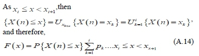
The frequency interpretation of F(x) and Xu follows: we perform the experiment n times and observe n values Xi,.. .,Xn random variables X [34]. If these numbers on the x-axis form the staircase function Fn(x); the steps are located at points xi, and their height equals 1/n [29]. It starts at the smallest value xmin of xi and Fn(x) = 0 for x < xmin.

The function Fn(x) is the empirical distribution of random variable X. For any specific X, the number of Fn(x) steps equals the number nx of xis smaller than X. Hence,

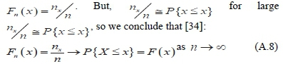
The empirical interpretation of the u percentile xu is the Quetelet curve. This derives from n line segments of lengths xi, separated vertically in order of increasing length, by distance 1/n. It forms the staircase function with corners at the endpoints of those segments.

Empirically, xu equals the empirical distribution of Fn(x), if the axes were interchanged. We know that [34]:

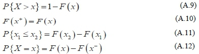
At a discontinuity, both the left and right-hand limits are different, and equation (A.12), becomes:

The only discontinuities of a distribution function Fn(x) are jumps, which occur at points xo where equation (A.13) is satisfied. Also, these points are listed as a sequence and can be counted [34]. The countable jump discontinuities [51] in Figure 2 were fifteen (15).

We deduce the staircase function using nonnegative real numbers corollary [34],[51]:

F(x) is a staircase function having an infinite number of steps, where i-th step size equals .

If F (χ) is constant except for a finite number of jump discontinuities, then χ is a discrete random variable. Such _x1 is a discontinuity point, and from equation (A.13), becomes [34],[52]:

The following Durbin-Watson statistic confirms the quality of interpretations of the study.

A.1.2. Durbin-Watson (DW) statistic

The 1.994 calculated Durbin-Watson (DW) statistic in model 4 (Table 3), was used for the model analyses [45]:

Decision rules for testing between the two hypotheses include: If D > du, we conclude Ho. If D > dL, we conclude Ha. If dL < D < du, DW test is inconclusive: where D is the computed DW value, du is the upper D limit, dL is the lower D limit, ρ is the autocorrelation parameter estimate, Ho is the null hypothesis, and Ha is the alternative hypothesis.

The DW statistic was evaluated using each residual value, et and its previous value, et-i [53],[54]:

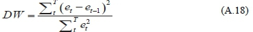
Where T is the number of time-series observations. Also, small D values indicate that ρ > 0 especially because neighboring error terms et and et-i have similar magnitudes, and are positively autocorrelated. If the residual differences et - et-i are small when ρ > 0, we have a small D numerator and a small test statistic.

Using parameters: k = 4; n = df + 1(32 + 1) = 33 and α = 0.05, where: df is the degree of freedom, η is the number of Cronbach's Reliability test predictors.

But, 4 - DW = 4 - 1.994 (= 2.006) > du (= 1.73).

So, we fail to reject the Null hypothesis. Thus, the goodness-of-fit closely mimics the electricity consumption and pricing model by 71.0%. The model is significant at 70.0% cut-off without autocorrelation effects or independent error assumption violations [54].

A.1.3. ANOVA

ANOVA partitions observed sample variance and the sum of squares into the minimum number of different significance tests to determine linear relationships between dependent and independent variables. Imperfect models have unexplained observed total variability [45],[49].

Basic regression line concept [50]: Data = Fit + Residual

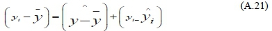
The first term in equation (A.21) is total y response variation, the second term is mean response variation, and the third term is the residual value.

Simplifying equation (A.21):

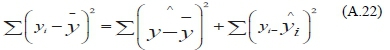
Equation (A.22) becomes: SSt = SSm + SSe, where SS is a sum of squares, T, M, and E, are total, model, and error symbols, respectively.

The sample square correlation is the ratio between the sum of squares and the total sum of squares: r² = SSm/SSt. Thus, r² is the variability fraction in the data explained by the regression model and sample variance [49],[50]:

MSm (model mean square) =

. The linear regression model has one variable X. Mean square error:

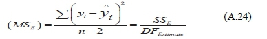
estimates variance about the population regression line _σ²

value tests hypothesis: against the^1.

null hypothesis: β = ο, βparameter estimates and F is Fisher-value). A test statistic is the ratio When

MSm is large, and the test ratio is large, there is evidence against the null hypothesis [23],[50].

Multiple linear regressions use ANOVA computations to adjust the minimum number of explanatory variables in the model [50]. The test statistic 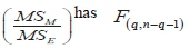distribution. The null hypothesis states: (b_i = b₂ = = β = θ), alternative hypothesis indicates at least one parameter , SSm/SSt = R², k = 0,1, q. However, F-test does not indicate which parameters are not zero. But, one parameter linearly depends on the response variable [50].

The ratio is the squared multiple correlation coefficient. Its square root is the multiple correlation coefficient R, and tests the relationship between observations yi and the fitted values yi [50].

 

II. APPENDIX B

B. I.ELECTRICITY LOAD MANAGEMENT QUESTIONNAIRE (PUBLIC)

Generally, electricity load management is the control of electricity consumption after the meter. This electricity consumption pattern involves several switching processes undertaken by the consumer. Consequently, it is to your advantage to be recognized as a resident in Namibia, which has an excellent reputation for quality housing development. Houses and building complexes are increasing in number, so also is the increasing need for satisfying electricity requirements.

In the light of the foregoing, therefore, we would like to please request you to give your candid opinion about efficient lighting and use of electricity in Buildings. We would also like you to please complete the following questionnaire with your permission, which we believe will not take more than fifteen minutes of your valuable time to answer.

Thank you for your willingness to cooperate by answering this questionnaire.

The questions follow:

1. Name: (Optional)...............

2. Respondents Gender: Male Female Age: 18-25, 26-35, 36-45, 46-55, Above 55

3. Region:..........Occupation......

E-mail ........Tel:..........

The key to answering the questions that follow in this questionnaire: SA-Strongly Agree A-Agree U-Not Sure DA-Disagree SD-Strongly disagree