A Spatio-Temporal Sleep Mode Approach to Improve Energy Efficiency in Small Cell DenseNets

 

 

Edwin Mugumet^I; Arthur Tumwesigye^II; Alexander Muhangi^II

^IDepartment of Electrical and Computer Engineering at Makerere University, P.O. Box 7062, Kampala, Uganda. Email: edwin.mugume@mak.ac.ug Member, IEEE
^IIDepartment of Electrical and Computer Engineering at Makerere University, P.O. Box 7062, Kampala, Uganda. Emails: {arthurtumwesigye1@cedat.mak.ac.ug; amuhangi}@cedat.mak.ac.ug

 

 

---

ABSTRACT

Data traffic has been increasing exponentially and operators have to upgrade their networks to meet the prevailing demand. This effort entails deploying more base stations (BSs) to meet the increasing traffic. The resulting capital expenditures (CAPEX) and operational expenditures (OPEX) have limited operator revenues. In addition to the energy costs, the associated greenhouse gas emissions have raised environmental concerns. In this paper, we use system-level simulations to investigate different sleep mode mechanisms that can address both capacity and energy efficiency (EE) objectives in dense small cell networks (DenseNets). These sleep mode approaches are applied to a long-term traffic profile that is obtained from real world network traffic. We then design a mechanism that determines the required BS density in response to the variable long-term traffic profile. Our results reveal that significant energy savings are possible when sleep mode mechanisms are applied based on the prevailing traffic in both time and space domains.

Index Terms: DenseNets, dynamic traffic, sleep mode, energy savings, energy efficiency.

---

 

 

I. INTRODUCTION

MOBILE traffic continues to increase exponentially due to high capacity devices and associated data hungry applications. A forecast of the global mobile data traffic shows a compound annual growth rate of 26% for the period from 2017-2022 [1]. Therefore, operators have got to continuously upgrade their networks to meet this spiraling traffic demand.

A typical approach to enhance network capacity is by making cells smaller which enhances the bandwidth per connected user. Significant small cell deployment creates an ultra-dense network of small coverage BSs; such a network is generally called a DenseNet in the research community [2]. In the era of 5G, small cells will become the core building blocks of the expected 5G heterogeneous networks. As is always the case, such dense small cell networks are designed to meet the prevailing peak traffic demand.

However, traffic highly varies in both the space and time domain. In the time domain, traffic peaks during the day i.e. during mid-morning, afternoon and early evening. Traffic falls off late at night, reaching its lowest level around 4am [3]. In the space domain, the traffic profile follows the daily movements of people, peaking in towns and city centers during the day and in residential areas during the evening hours. Since mobile networks are designed to meet peak traffic under certain constraints, the spatio-temporal variation of traffic leaves many cells idle during low traffic periods or in low traffic areas.

In order to enhance the energy performance of the network, the network should be designed to minimize the absolute power it consumes or maximize its energy efficiency (EE). Given the variation of traffic, this can only be achieved if the energy consumption of the network dynamically changes with traffic demand [4]. Sleep modes are the most popular of the proposed approaches to achieve this dynamic adaptation of energy consumption to the prevailing traffic conditions. In other words, some appropriate base stations (BSs) can be switched off when traffic is low and the remaining BSs can serve the active users.

Authors in [5] discussed how sleep mode schemes can be successfully used to manage power consumption through switching off some BSs and using remaining active BSs to balance the prevailing traffic load. The work in [4] also showed enhanced energy performance when a sleep mode strategy that puts focus on cells with the fewest users for sleep mode is followed. However, given that the traffic load is highly dynamic in space and time, switching the BSs on and off can prove to be counterproductive. Therefore, it is important to develop long-term and short-term strategies that can keep certain BSs off for a significant period while allowing the remaining BSs to still respond to short-term traffic variations.

Previously, mobile networks have been designed with the objective of optimizing coverage, capacity, spectral efficiency or throughput. This does not necessarily maximize energy efficiency (EE) as expected. This makes green networking an interesting and technically challenging research field. Therefore, a new energy conserving approach is needed so that existing DenseNets will maintain the same level of quality of service (QoS), reduce operational expenditures (OPEX) and environmental degradation while reducing the amount of energy consumed in the future [6].

In this paper, we study appropriate sleep mode strategies in DenseNets. Network performance is characterized using coverage, rate and energy metrics. We investigated the performance of our proposed sleep mode mechanism and compare it with two common approaches from literature. Our results show that the proposed sleep mode scheme maximizes energy savings and network EE.

A. Paper Organisation

The rest of the paper is organized as follows. Section II discusses the main assumptions used and the system model.

Section III analyzes the dynamic traffic profiles and their effect on energy consumption. Section IV discusses the network performance metrics based on the interaction between the users and small BS densities. Section V discusses the various sleep mode approaches used to determine the BSs requirement. Section VI presents and discusses the numerical results of the analysis. The paper is then concluded in Section VII.

 

II. System Model

In this section, we describe the proposed network layout, the channel model and the power consumption model of BSs.

A. Network Layout

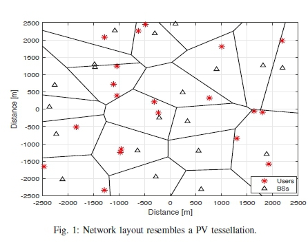
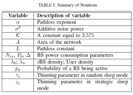
We consider a DenseNet of small base stations (sBSs) which are deployed over a square area A, and each transmits the same nominal power P_t. The sBSs and users are deployed according to two independent homogeneous Poisson Point Processes (PPP) Φ₈ and Φ„ of densities λ_band λ_urespectively. The network environment is described using a path loss exponent α. The network layout resembles a Poison Voronoi (PV) tessellation [7] as shown in Fig. 1. In addition, we consider universal frequency reuse without loss of generality. Table I lists the common notations used in this paper.

 

 

 

 

B. Channel Model

In the channel model, long-distance path loss, fading and additive noise are considered. The path loss is modeled as PL(d) = Ld^-a, where d is the propagation distance and L is a path loss constant. Random channel effects are incorporated by a Rayleigh fading factor h of unit mean [8]. Therefore, the power received by the typical user at a distance d from its serving sBS, denoted as P_r, is expressed as P_r(d)= P_thLd^-a.

Given universal frequency reuse, a typical user receives interference from all sBSs other than its serving sBS, denoted as b₀. The Signal-to-Interference-plus-Noise Ratio (SINR) of the typical user is therefore expressed as

 

 

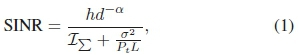
where is the aggregate interference, g_iis the fading loss between the typical user and the i-th interfering sBS, d_iis the distance between the user and the i-th interfering sBS, b_idteis the set of sBSs that remain idle after cell association, and σ² is the additive noise power. Both h and gi are assumed to be independent identically distributed (i.i.d) exponential, where

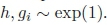
C. Power Consumption Model

An idle BS consumes only static power. If a BS is put to sleep mode, not only is the transmit power zero but also some of its components are switched off hence reducing its static power. It is desirable for a BS in sleep mode to be completely switched off for a given period to save energy. In this paper, we devise a mechanism of predetermining this period to maximize energy savings. Typically, a sBS can be in active mode where it has at least one user, idle mode where it has no users, sleep mode or be completely switched off. According to [9], the power consumed by a BS in the different states of operation, denoted as P_c, is generally expressed as

 

 

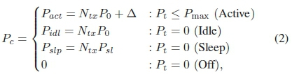
where N_txis the number of transceiver chains, N_txP₀is the consumed static power, Δ is the slope of the load-dependent power consumption, P_s¡ is the power consumed by each transceiver chain in sleep mode, and P_max is the maximum RF output power. Note that making sleep mode power consumption much less than idle mode power consumption. The parameter values for different BS types are in [9]. We evaluate the energy performance using Area Power Consumption (APC) and EE. The APC in Watts/m² is calculated as

 

 

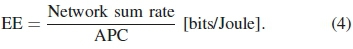
where On the other hand, the EE depends on the network sum rate which is a sum of all the capacity achieved by all users in the network. The network sum rate is dependent on the sleep mode approach and will be analyzed later in paper. EE is therefore calculated as

 

III. Dynamic Traffic Profiling

In this section, we analyze the dynamic nature of the daily traffic profile and demonstrate its possible effect on the energy performance of a typical cellular network. In general, traffic varies spatio-temporally throughout the day [10]. In the time domain, traffic peaks during the day (mid-morning, afternoon and early evening) and then tails off after midnight. In the space domain, the traffic profile follows the daily movements of people, peaking during the day in townships and city centers and in residential areas during the evening. Whereas the network is dimensioned to meet these peak traffic levels, network BS planning cannot easily adapt to these daily spatio-temporal traffic variations. As a result, many BSs which are active during peak traffic periods inevitably become idle when traffic reduces. However, often, these BSs continue to consume energy even when idle. Therefore, in order to make cellular networks more energy efficient, there is a clear need to adapt their power consumption to the dynamic nature of the prevailing traffic profile.

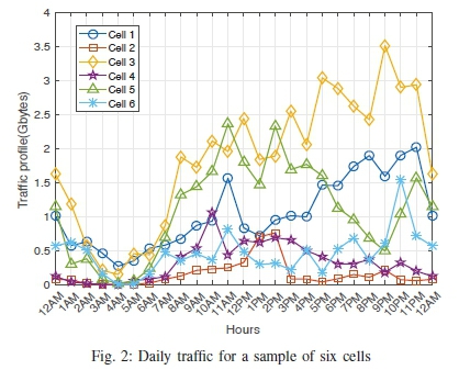
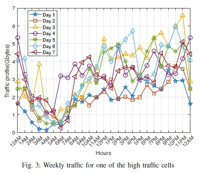
In this analysis, we use actual traffic data obtained from a major mobile network operator in Uganda. The data belongs to various neighboring cells located in a cluster in an urban area. Fig. 2 shows the traffic profile from a sample of six cells. It demonstrates the spatio-temporal variation of traffic in the following ways: (a) in the time domain, minimum traffic is generally recorded between 2am and 7am in all the cells. Whereas the peaks vary from cell to cell, they tend to be in the early afternoons or late evenings; (b) in the space domain, some cells carry more traffic than others, usually as a result of the prevailing spatial distribution of cellular users. This spatial variation prevails even though these cells are from the same neighborhood. Spatial variation is even more pronounced between urban, suburban and rural areas. Fig. 3 shows the recorded traffic for one of the high capacity cells over one week period. It shows that the traffic profile is different for each day and is not straightforward to accurately predict.

 

 

 

 

The dynamic nature of the traffic in Figs. 2-3 provides an opportunity to save energy, especially during low traffic periods. Sleep mode mechanisms are a popular approach to adapting network power consumption to the prevailing load conditions. The traditional approach to sleep mode mechanisms has been to vary the density of active BSs as the traffic varies in space and time. However, BSs take a finite time to switch on and off and it is hard to vary their density fast enough to keep up with the rapid traffic variation. In addition, the required rapid switch on and off of BSs is resource intensive and can be rather counterproductive. The reasonable approach is to determine an approximated traffic profile with similar traffic over reasonable periods of time. Over these periods, the instantaneous variation of traffic is essentially limited within tight bounds and a BS density can be predetermined to support this traffic. In addition, any other unrequired BSs can be switched off, saving considerable energy and adapting energy consumption to the traffic profile.

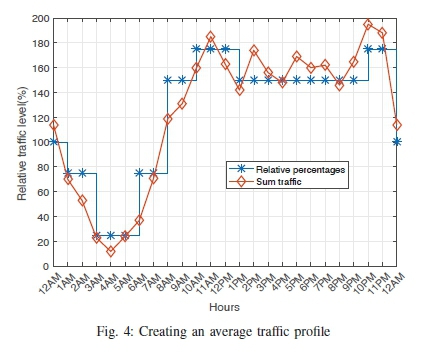
Fig. 4 shows the sum of all the traffic in the considered 6-cell cluster over a period of 2 months. Using the sum traffic removes spatial and temporal biases over the period to give a fairly average traffic profile over this cluster. Using the average sum traffic profile, scalar quantization is used to map the "analog" values of the traffic to a common value within a specific range of time. This yields five constant traffic segments spanning appropriate time periods as seen in Fig. 4. Generally, these segments can be mapped on a percentage scale [10], with the appropriate middle segment considered as the 100%-segment. As shown in Fig. 4, the middle segment is mapped to 100% and the lower and upper segments are also mapped appropriately. These segments can be used to predict the required number of BSs that can support each traffic segment. By finding the required number of BSs to meet the traffic per segment, it becomes possible to quantify the energy savings from long-term sleep mode.

 

 

In this paper, we assume that during the maximum traffic segment, all the sBSs are required but as traffic reduces in other segments, some sBSs can be put to sleep mode or switched off completely to save energy. After user association among the remaining sBSs, some sBSs will be active while others will remain idle. The idle BSs can be put in conventional sleep mode where they consume less energy. Note that in this sleep mode state, the switch on time is shortened should a sBS be required to support mobile users. If the next traffic segment is higher, a predictable number of sBSs are switched on as the current segment nears its end. However, if the next segment is lower, extra BSs from among the available sBSs are also switched off.

 

IV. NETWORK PERFORMANCE ANALYSIS

In this section, we introduce the three sleep mode strategies that we considered in this paper. We analyze the performance of these approaches in terms of energy consumption and energy efficiency. However, we start this section by analyzing the SINR coverage and spectral efficiency performance of the network as a function of the interaction between the prevailing user and sBS densities. This analysis considers the fact that after user association, some sBSs may remain idle, the density of which depends on the user density in the network.

A. SINR Coverage Probability

The probability that a typical user receives SINR greater than a given threshold is an important measure that greatly impacts the quality of service. SINR coverage probability, denoted as P_cov, is therefore defined as

where T_cis the SINR coverage threshold. According to [11], P_covis expressed as

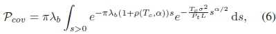
where . The analysis in this work is based on the assumption that , such that each sBS associates with at least one user.

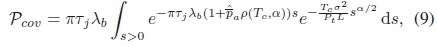
This assumption is not realistic in practical networks where some sBSs inevitably remain idle after cell association. For example, in Fig. 5, there are some idle BSs caused by the independent distributions of sBSs and users. The analysis in [12] considers the thinning effect of idle sBSs on the aggregate interference, and expresses P_covas follows:

 

 

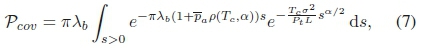
where is the density of all active sBSs less the serving sBS (an active sBS is one that covers at least one user). In other words, if all active sBSs are , where p_ais the probability that a typical sBS is active, then . Note that the density of idle sBSs in (1) is .

In [12], pa is shown to depend on the interaction between users and sBSs, and is expressed as

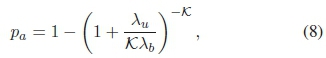
where K = 3.575 [7] is a constant. For example, it can be seen from (8) that as , which verifies the assumption in [11].

Since traffic varies, it is possible to independently thin the network so that some sBSs can be switched off for some time. According to Fig. 4, each constant traffic segment requires a set of sBSs to serve that traffic, and the remaining sBSs can be switched off for that time period. In such a case, in order to easily change the sBS density for each traffic segment, we simply vary a parameter , where and N_tis the number of segments in the traffic profile.

According to Slivnyak's theorem [13], an independently thinned PPP is also a PPP. Based on this principle, (7) is modified as follows:

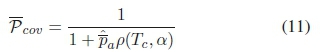
where is the prevailing sBS density of the concerned segment and is the active sBS probability, now expressed as

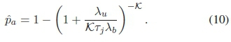
Note that .

Proof. In (7), instead of using the sBS density as , replace it with

In an interference-limited network, and SINR SIR i.e. . Hence, (9) simplifies to

This defines the upper bound on the coverage performance of the network since presence of noise only reduces P_covfurther.

B. Rate Coverage Probability

Similarly, the rate coverage, denoted as P_rate, is defined as

where T_ris the rate coverage threshold. In this case, P_rateis essentially the probability that a typical user achieves a target rate of Tr [bps/Hz]. Generally, the probability of rate coverage is expressed as

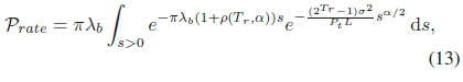
where

Proof. Note that (12) can be restated as

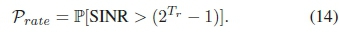
Hence (5) and (12) are of the same form. In (6), we replace . ■

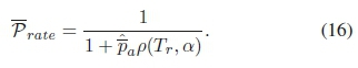
Due to the independent distribution of sBSs and users, some cells remain idle and do not contribute interference. Considering this and the effect of independent thinning, (13) can be modified to have the same form as (9) as follows:

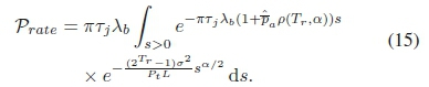
The interference-limited network, where , defines the upper bound on rate coverage probability. Hence, (15) simplifies to

C. Network Spectral Efficiency

In [12], the average spectral efficiency (SE) per connected user in the network is expressed as

Assuming that each sBS serves one user at a time, the number of connected users is equivalent to the number of active sBSs. Therefore, the number of served users, denoted as , where is the proportion of all users that get served, is expressed as . Since the average user SE and number of connected users are known, the average sum SE is expressed as

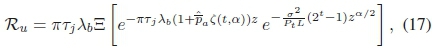
Since R_sper segment is already known, we seek to determine the sBS density that achieves this capacity. It is not possible to express (18) in closed form in terms of X_b. Therefore, we use the bisection method [14] to find the required sBS density of the j-th traffic segment, denoted as

 

V. Sleep Mode Approaches

To verify our analysis, we use the sleep mode schemes presented in [12]. Using each of the three schemes, we determine the required sBS density for each traffic segment. In this paper, we briefly discuss the three schemes for completeness.

A. Conventional Sleep Mode

This is a basic sleep mode scheme where only idle sBSs are put to sleep after user association to save energy. The sBSs in sleep mode can be required at any time as users move around the network. No sBSs are switched off completely during the different traffic segments. Since all sBSs are available for user association, each user associates to its ideal serving sBS. The idle sBSs, which are put to sleep, thin the aggregate interference suffered by the typical user, hence enhancing SINR. Fig. 5 shows conventional sleep mode in the network. Compared to Fig. 1, it can be seen that idle sBSs have been removed from the active set and the remaining active sBSs have expanded their coverage to cover the whole service area. Comparing the segments, a low traffic segment will require fewer active sBSs than a high traffic segment to meet the target traffic.

In practice, due to mobility, sBSs can become idle momentarily. In such cases, this scheme requires sBSs to switch on and off rapidly and frequently, which can be counterproductive in terms of quality of service. The SINR coverage probability in (7) is based on conventional sleep mode. The idle sBS density that goes to sleep is (1 - p_a)X_b. Hence, the power consumed by the network is expressed as

B. Random Sleep Mode

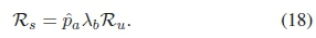
In this scheme, the density of sBSs that meet the traffic of a given segment is determined by varying Tj, using the bisection method, to satisfy (18). Since changing Tj results in independent thinning of the network, normal user association takes place within the remaining sBS density TjXb. Random sleep mode follows Algorithm 1.

 

 

Initially, the sBS density (1 - Tj)Xb, which is not required during the j-th segment, is switched off for the entire segment to save energy. However, after cell association, some extra sBSs may remain idle and will be put to sleep. Therefore,

the respective densities of active and idle sBSs are p_a X_band (1 -p_a)X_b. The power consumption becomes

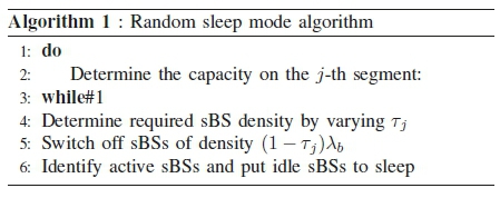
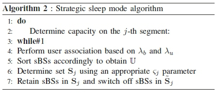
C. Strategic Sleep Mode

In strategic sleep mode, the number of sBSs required per segment is chosen based on a criteria that perceives the importance of a sBS to the network. In [12], the criteria is that sBSs which associate with the most users are perceived to be more important. As a justification, fewer users are disrupted by switching off their parent sBSs. Clearly, this approach prioritizes idle sBSs first.

Define set as the set of all sBSs such that . Now consider a parameter , where , that corresponds to the j-th traffic segment. Then, by varying , we can determine the set of sBSs, denoted as , that satisfies the traffic of the j-th segment i.e. . The set of sBSs that are switched off, denoted as Sj, is expressed as . Strategic sleep mode follows Algorithm 2.

 

Depending on the sBS and user densities prevailing during a given traffic segment, it is possible that Sj also contains some idle users. If this is the case, those idle sBSs are also put to sleep mode. Let Sj = Sj, _act U Sj_¡idle, where Sj_actand Sjidie are the respective sets of active and idle sBSs in Sj. The power consumption the j-th segment becomes

In this section, the numerical results are presented to evaluate the ability of the sleep mode mechanisms to adapt network energy consumption to the prevailing load conditions. Unless otherwise stated, the simulations are based on the default parameters shown in Table II.

 

 

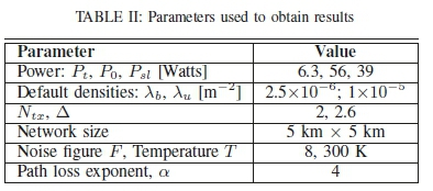
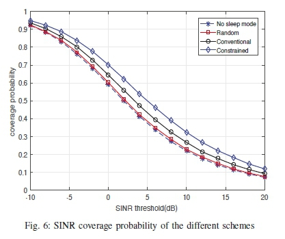
Fig. 6 shows the variation of the SINR coverage probability with the target SINR threshold. The "no sleep mode" case, in which all sBSs are active such that the aggregate interference is maximized, is the worst case scenario and provides the lower bound on the SINR coverage probability performance. Random sleep mode only gives negligible improvement over the lower bound due to its random selection of sleep mode BSs. Due to this random selection, sometimes sBSs with many users will be put to sleep, affecting many users whose SINR will deteriorate as they have to connect to new but more distant 'parent' sBSs. The conventional scheme performs significantly better than random sleep mode because SINR generally improves for two reasons: (a) the received power is not affected; and (b) aggregate interference reduces once idle BSs are put to sleep. The constrained scheme has the best performance due to two main reasons: (a) a larger number of BSs can be put to sleep mode, reducing the aggregate interference significantly; and (b) since BSs with the least users are prioritized for sleep mode, the number of users whose received power is affected by sleep mode is minimized. The combination of these two scenarios results in enhanced SINR coverage.

 

 

Similar to the SINR coverage probability, the rate coverage probability also originates directly from the average SINR performance of each sleep mode scheme. Therefore, as shown in Fig. 7, constrained sleep mode gives the best average rate performance while random sleep mode does not show any significant improvement over the 'no sleep mode' case that defines the lower bound on performance. For example, for a rate threshold of 2 b/s/Hz, the rate coverage probabilities are 0.38, 0.4, 0.45 and 0.5 for no sleep mode, random sleep mode, conventional sleep mode and constrained sleep mode respectively.

 

 

As explained earlier using Fig. 4, we predict the required number of sBSs to meet the prevailing demand for each traffic level segment. The constrained and random sleep mode schemes will need different sBSs to achieve the given traffic level.

Fig. 8 shows the daily power consumption of the network based on the required number of sBSs. Note the following important points:

1) Generally, conventional sleep mode consumes the most absolute power because only idle BSs are put to sleep. In addition, constrained sleep mode minimizes absolute power consumption because it maximizes the traffic derived from each active BS. However, random sleep mode consumes less power than its conventional counterpart because due the random selection of BSs for sleep mode, some selected BSs will remain idle and can be put to sleep to save more energy.

2) The higher the prevailing traffic level, the more the power consumption since more BSs are required to meet the high traffic demand.

3) During the peak traffic period (the 175% segment), the three schemes consume the same amount of power. This is due to our assumption that the network is planned such that during the busy hour, all the BSs are required and there is no need for sleep mode.

4) During low traffic periods, power consumption reduces but there is a smaller difference between the schemes because they can all support the low traffic using very few BSs. However, as traffic demand increases, the constrained sleep mode algorithm begins to provide significant advantages over random and conventional algorithms.

 

 

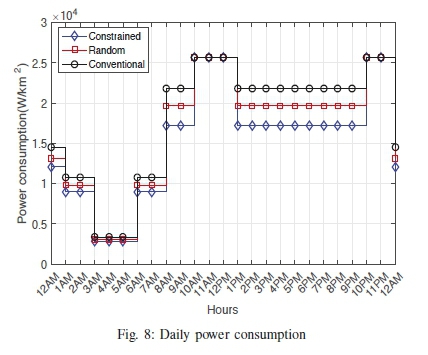
Fig. 9 shows the daily energy savings derived from implementing the three sleep mode schemes. Generally, there is no energy saved at peak traffic since all BSs are required and only idle BSs are put to sleep (i.e. conventional sleep mode). As traffic begins to decrease however, constrained and random sleep modes can be used to save significant energy. For example, constrained sleep mode gives an energy saving of 40.9% over the entire 24-hour day compared to random and conventional schemes which give 35.5% and 30.4% respectively. In general, energy saving is maximized during low traffic segments but at high traffic, there is no significant difference between the different sleep mode schemes (as explained in Fig. 8).

 

 

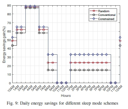
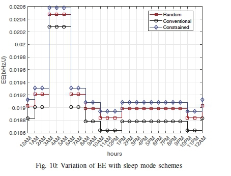
Fig. 10 shows the EE performance of the network using the three sleep mode schemes. The main result to note is that constrained sleep mode has a better EE performance than random sleep mode since it saves more energy. The overall weighted average EE of constrained sleep mode over the entire 24-hour day is 0.0193 b/Hz/Joule compared to 0.0191 b/Hz/Joule and 0.0187 b/Hz/Joule for random and conventional schemes respectively. This is a significant performance improvement especially at high bandwidths. For example, assuming a bandwidth of 10 MHz, the EE performance improvement of the constrained scheme over the random and conventional schemes is 2 kb/Joule and 6 kb/Joule respectively. Note that at peak traffic, all the schemes resemble the conventional scheme since all BSs are available to carry traffic.

 

 

 

VII. Conclusion

Traffic forecasts show that traffic demand will continue to increase exponentially in future. Mobile operators are faced with increasing costs of expanding and maintaining their networks to meet this increasing traffic demand. Energy is the biggest component of OPEX and significantly shrinks operator revenues. In this paper, we proposed a sleep mode scheme called constrained sleep mode to adapt energy consumption to the prevailing traffic in the network. Our proposed scheme outperforms comparable schemes from literature in terms of energy savings and energy efficiency (EE). Constrained sleep achieves its better performance by prioritizing BSs with the least number of users as candidates for sleep mode. This minimizes the number of disrupted users which maintains a better average SINR compared to the other schemes.

 

References

[1] Cisco, "Cisco Visual Networking Index: Forecast and Trends, 2017-2022 White Paper," Cisco Systems.Inc, Document ID:1551296909190103 (updated March 9, 2020).

[2] Qualcomm Inc., "The 1000x Mobile Data Challenge," White Paper, November 2013.

[3] M. Marsan, et al, "Optimal Energy Savings in Cellular Access Networks," IEEE International Conference on Commununication Workshops, pp. 1-5, June 2009.

[4] E. Mugume and D. K. C. So "Sleep Mode Mechanisms in Dense Small Cell Networks," 2015 IEEE International Conference on Communications (ICC), London, 2015, pp. 192-197.

[5] L. Xiang, et al, "Adaptive traffic load-balancing for green cellular networks," 2011 IEEE 22nd International Symposium on Personal, Indoor and Mobile Radio Communications, Toronto, ON, 2011, pp. 41-45, doi: 10.1109/PIMRC.2011.6139995.

[6] A. Gopal and D. Sunehra "A survey on Energy Efficient Base Station Sleeping Techniques in Green Communications," in 2017 Telengana India.

[7] E. Pineda, and D. Crespo, "Temporal Evolution of the Domain Structure in a Poisson-Voronoi Nucleation and Growth Transformation," Physical Review E, American Physical Society, 2008.

[8] J. G. Andrews, A. K. Gupta, and H. S. Dhillon, "A Primer on Cellular Network Analysis Using Stochastic Geometry." CoRR in ArXiv, 2016.

[9] G. Auer, et al., "How much energy is needed to run a wireless network?", IEEE Wireless Communications, vol. 18, no. 5, pp. 40-49, October 2011.         [ Links ]

[10] O. Blume, A. Ambrosy, M. Wilhelm and U. Barth, "Energy Efficiency of LTE networks under traffic loads of 2020," The Tenth International Symposium on Wireless Communications Systems, Iimenau, Germany, 2013, pp. 1-5.

[11] J. G. Andrews, F. Baccelli, and R. K. Ganti, "A Tractable Approach to Coverage and Rate in Cellular Networks," IEEE Transactions on Communications, Vol.59(11), pp. 3122-3134, Nov 2011.         [ Links ]

[12] E. Mugume and D. K. C. So, "Deployment Optimization of Small Cell Networks With Sleep Mode," IEEE Transactions on Vehicular Technology, Vol.68(10), pp. 10174-10186, Oct. 2019.         [ Links ]

[13] M. Haenggi et al., "Stochastic Geometry and Random Graphs for the Analysis and Design of Wireless Networks," IEEE Journal on Selected Areas in Commun., Vol. 27(7), pp. 1029-1046, Sept 2009.         [ Links ]

[14] R. L. Burden and J. D. Faires, Numerical Analysis: Bisection Method, 9th Ed., Brooks/Cole, Cengage Learning, 20 Channel Center Street, Boston, MA 02210, USA, 2011.

 

 

Edwin Mugume (S'12-M'17) received the Bsc degree in Electrical Engineering (First Class Honours) from Makerere University, Uganda in 2007, and the Msc degree in Communication Engineering (Distinction) from the University of Manchester, United Kingdom in 2011. He completed the PhD degree in Electrical and Electronic Engineering from the University of Manchester, UK in 2016.
From 2008 to 2010, he was a radio planning and optimization engineering engineer for cellular networks at Nokia Siemens Networks and Bharti Airtel. He is currently a lecturer in the Department of Electrical and Computer Engineering, Makerere Univeristy. His research interests include energy efficient dense heterogeneous networks, 5G cellular technology, and application of machine learning in wireless networks and systems.

 

 

Arthur Tumwesigye received the Bsc (First Class Honours) degree in Telecommunications Engineering from the Department of Electrical and Computer Engineering in Makerere University, Uganda in 2020.
He is currently working as a network engineer at the Research and Education Network for Uganda (RENU). He received the best paper award for his scholarly contributions in the 2019 National Conference on Communications held in Kampala, Uganda. His research interests include Iterative Detection and Decoding (IDD) algorithms, 5G cellular technologies, Energy Efficient dense networks and Machine Learning applications in cellular systems.

 

 

Alexander Muhangi received the Bsc (Hons) degree in Telecommunications Engineering from Mak-erere University, Uganda in 2018, and enrolled for his Msc degree in Telecommunications Engineering from Makerere University, Uganda in 2019.
From 2017 to 2019, he worked as a quality of service engineer in the radio network planning and optimization department of Africell Uganda. He is currently a graduate researcher in netLabs!UG under the Department of Electrical and Computer Engineering, Makerere Univeristy. His research interests include 5G cellular technologies, Green Wireless Technologies, Machine learning driven wireless networks and systems, Data Analytics, and Internet of Things (IoT).