ARTICLES

 

Pareto Design of Decoupled Fuzzy Sliding Mode Controller for Nonlinear and Underactuated Systems Using a Hybrid Optimization Algorithm

 

 

Mohammad Javad Mahmoodabadi^I; Rahmat Abedzadeh Maafi^II; Shahram Etemadi Haghighi^III; Abbas Moradi^IV

^IDepartment of Mechanical Engineering, Sirjan University of Technology, Sirjan, Iran (e-mail: mahmoodabadi@sirjantech.ac.ir)
^IIDepartment of Mechanical Engineering, Science and Research Branch, Islamic Azad University, Tehran, Iran (e-mail: meysam.abedzade@yahoo.com)
^IIIDepartment of Mechanical Engineering, Science and Research Branch, Islamic Azad University, Tehran, Iran (e-mail: setemadi@srbiau.ac.ir)
^IVDepartment of Mechanical Engineering, Takestan Branch, Islamic Azad University, Takestan, Iran (e-mail: abbasmoradi88@gmail.com)

 

 

---

ABSTRACT

This paper introduces Pareto design of the decoupled fuzzy sliding mode controller (DFSMC) based on a hybrid optimization algorithm for a number of fourth-order coupled nonlinear systems. In order to achieve an optimal controller, at first, a decoupled fuzzy sliding mode controller is utilized to stabilize the fourth-order coupled nonlinear systems around the equilibrium point. Then, a robust hybrid optimization algorithm is employed to enhance the capabilities of the control system. The mentioned algorithm is an optimal combination of artificial bee colony (ABC) and bacterial foraging (BF) algorithms enjoying the advantages of both. To evaluate this algorithm and to challenge its capabilities, firstly, the required test functions and evaluation criteria have been defined, and then, the results have been compared to those of the well-known algorithms including NSGAII, SPEA2 and Sigma MOPSO. The comparison illustrates the superiority and more accurate performance of this novel hybrid algorithm. Moreover, juxtaposition of Pareto solutions offered by the proposed method and the true optimal Pareto front demonstrate that the proposed algorithm is able to accurately overlap the true solutions. Eventually, by simulating three nonlinear systems, i.e. the inverted pendulum, ball and beam, and seesaw via MATLAB software and choosing proper objective functions, the coefficients of control law for both decoupled sliding mode and decoupled fuzzy sliding mode controllers are optimized so as to reach the most optimal performance for these dynamic systems. Simulations indicate that the decoupled fuzzy sliding mode controller surpasses the non-fuzzy counterpart in terms of accurately controlling the aforementioned systems. This technique can optimally stabilize the system states at their equilibrium points in a relatively short time. Besides, in order to validate the solutions obtained in this paper, they are compared with previous works.

Index Terms: artificial bee colony, bacterial foraging, decoupled fuzzy sliding mode, multi-objective optimization, Pareto design, sliding mode control, underactuated system

---

 

 

I. Introduction

THERE have been numerous control methods to inspect the control behavior of nonlinear systems [1-9] among which sliding mode control is renowned as a prominent technique for controlling these systems due to its significant advantages such as robustness to parameters change, rapid dynamic response, stability assurance, external noise repelling, and the simplicity in design and implementation [1]. Although the sliding mode controller can control second-order systems favorably, this feature is not simply feasible for the fourth-order coupled systems [10]. As a resolution to this problem, such systems can be converted to the canonical form on which the sliding mode controller is perhaps applicable. However, this conversion includes the disadvantage of heavy calculations. The other solution is to utilize the decoupled sliding mode sample. In this method, the decoupled sliding mode theory can be applied without converting the system to its canonical form [11]. Nevertheless, the discontinuous behavior of sliding mode controllers, when system states reach the sliding surface, causes the undesirable chattering phenomenon [12, 13].

Another method to control nonlinear systems is the fuzzy control. Theories of fuzzy logic and fuzzy sets were first presented by Zadeh [14,15]. Fuzzy systems have been applied in many fields of science such as control, medicine, economics, management, business and psychology. However, the bulk of the studies and experiments have been implemented in the field of control [16-23]. Fuzzy control is mostly used in complex, badly defined, non-linear, and time-variable systems.

Fuzzy rules can provide simple conditions for controlling a variety of dynamic systems. This simplicity is due to the fact that fuzzy controllers do not usually require a precise mathematical model of the controlled system. In recent years, the combination of sliding mode and fuzzy controllers has

In order to maximize the quality of controllers and the performance of a dynamic system, control coefficients can be optimized by selecting proper objective functions so that the design objectives are well-met. Nonetheless, it should be noted that when it comes to complicated structures and constraints along with multiple contradictory objectives, solving optimization problems through classical and analytical methods, may be arduous and in some cases unfeasible [33]. In this state, evolutionary algorithms can play a significant role. Some of the most acknowledged algorithms are genetic algorithm (GA) [34-38], particle swarm optimization (PSO) [39-43], artificial bee colony (ABC) [4450], bacterial foraging (BF) [51-54], simulated annealing (SA) [55-57], and cockroach colony optimization (CCO) [58, 59] which are all numerical methods inspired by nature. Each of these algorithms has its own strengths and weaknesses due to its unique qualities. Recently, in order to better exploit the strengths and to abate the weaknesses, various combinatorial algorithms have been introduced [60-67]. In this study, a hybrid optimization algorithm, presented in [65] is utilized to optimize control problems. In the methodology, ABC and BF algorithms are optimally combined and have yielded a novel and practical hybrid algorithm for solving optimization problems in both single-objective and multi-objective areas.

 

II. Optimization

Optimization is simply known as a branch of mathematics and computation science which studies the methods to find the best answer for an optimization problem. The optimization theory investigates the quality of spotting the best answer, and therefore, detecting the more optimal as well as valuation of desirable and undesirable must be well defined. This theory is about investigation of the optimum points and the methods for finding them [68]. The optimal answer of an optimization problem is the extremum of its objective function. In most cases, the problem would be regarded as a minimization problem, without lacking integrity. Thus, the optimal resolution of an optimization problem is the point which minimizes the objective function, and the ultimate purpose of optimization is to find such a point. The objective function, on the other hand, constitutes the item that needs to be optimized, and is classified into single-variable and multi-variable. These variables, also known as decision variables or optimization parameters, should be explored using optimization techniques so that the objective function is optimized.

Optimization problems can be expressed in different forms based on the number of objective functions, properties of the functions, constraints, and others [69]. In the following, the problems are classified with respect to their objective functions.

A. Single-Objective Optimization

A single-objective optimization problem, as it reveals, has only one objective function to be optimized. This function, however, can hold several decision variables. A single-objective optimization problem can generally be expressed as follows: been in the center of attention of many researchers [24-32].

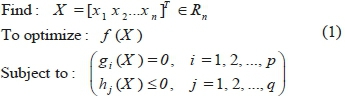
in which, f (X) represents the only objective function, χindicates the decision variable vector, g is the equal constraint, and h shows unequal constraints.

B. Multi-Objective Optimization

In the majority of optimization problems, more than one objective function is regarded by designers. In such problems, two or more contradicting objectives need to be optimized simultaneously. The standard form of a multi-objective optimization problem is as follows:

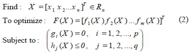
where F(X) is the objective function.

Unlike the single-objective problems which contain only one optimum point, the multi-objective optimization problems lead to finding a series of optimum points which are not superior to each other. In this set of problems, dissimilar to single-objectives, a collection of design vectors is obtained as the final answer called the Pareto points. The designer can select any of these points as the optimum answer respecting the requirements of design.

 

III. Artificial Bee Colony and Bacterial Foraging

Artificial bee colony (ABC) algorithm was first introduced by Karaboga on the basis of the exploring behavior of honey bees. In this method, each of the bees tries to obtain the best solution, respecting probability laws, through direct interacting and sharing information. In this algorithm, the locations of new food resources are determined using the following equation:

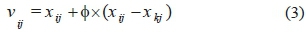
where φ is a random number between 1 and -1; i and j indicate the number of position and the number of food resource, respectively; and k is also generated arbitrarily and differs from i .

The original concept of bacterial foraging (BF) algorithm is based on the fact that in nature, organisms equipped with poorer foraging approaches are more prone to distinction than those having stronger foraging strategies. Passino [51], as well as Liu and Passino [52] proposed the BF algorithm, inspired by the foraging behavior of bacterium Escherichia coli (E. coli) in human intestine, as a novel solution to optimization problems. This algorithm stands on four stages.

A. Chemotactic

In this phase, each bacterium picks a route for its maneuver. If a bacterium detects a better food source on the new route, it tends to move in that direction (swimming motion).

B.Swarming

When a bacterium discovers a better route for more food, it attracts other bacteria to take the route more easily as a group.

C.Reproduction

Half of the bacteria that didn't succeed to reach food die and the other half will split into two bacteria.

D.Elimination and dispersal

This stage prevents the bacteria from being trapped in local optimum points. Each bacterium is in danger of elimination and dispersal with the probability of P_ed, in each iteration.

New food source location in this algorithm is determined as:

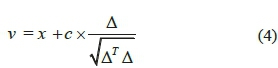
in which, v and x indicate new and old food source locations, respectively; c is a constant and equals to 0.01; δis a unit vector having the same dimension as X , and each of its components is a random number between -1 and 1.

 

IV. The Proposed Optimization Algorithm : ABC in Conjunction with BF

The purpose of this algorithm which is a combination of ABC and BF is to utilize the merits of both algorithms and to introduce a novel and robust one so to tackle multi-objective optimization problems. The details of this novel algorithm are as follows stages:

Stage 1.

An initial population is arbitrarily generated regarding the domain and dimension of the problem using the following equation:

where x ^max and x ^min are the upper and lower bounds for design variables. At this stage P_edand N_smust be set, which in here are taken as 0.25 and 3, respectively. P_eddenotes the elimination probability of member i , while its second random selection defines the domain of the problem. N_s, on the other hand, determines the number of admissible swimming stages. Note that, responses related to the initial population are calculated in this stage.

Stage 2.

This stage happens in a repeat loop and it doesn't cease unless the number of iterations reaches its maximum:

a. Selecting half of the population arbitrarily and determining their new locations using ABC algorithm employing equation (3): In this stage if the new location surpasses the previous one, the former replaces the latter.

b. Selecting the other half of the population and setting new locations for them based on the BF algorithm as in equation (4).

c. Replacing the inferior half by the superior member of the whole population.

d. Elimination and dispersal operation for all members of the population.

Stage 3.

Announcing the best member among the whole population and the solution resulted from it.

 

V. The Proposed Multi-Objective Optimization Algorithm: ABC in Conjunction with BF

in order to utilize the proposed algorithm in multi-objective optimization operation, the following steps are implemented:

A.Detecting the Non-Dominant Solutions and Saving Them in the Archive

in each iteration, a set of solutions which are not superior to each other are collected in the archive.

B.Limiting the Archive via Neighborhood Radius

If all the non-dominant solutions are stored in the archive, then soon it will expand in size and causes dullness in the algorithm performance. In this study, a technique called neighborhood radius has been employed to prune the archive. Each of the available solutions is supposed to have a radius r. According to this technique, if the Euclidean distance between two answers falls shorter than r, one of them will be eliminated.

C.Using the Sigma Method

in this method, each member selects a response from the archive as its best response in each iteration. At first, the sigma equation is calculated for all the members of population together with all the archive members. Then, the absolute distances between each member's sigma and the sigma of all archive members are calculated. The lowest value shows the member of the archive with the best response. The following equation shows how this step works:

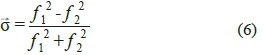
where, f ₁ and f ₂ indicate the first and second objective

functions. The latter equation is mostly utilized for two-objective optimization problems. However, it can easily be extended to problems with more than two objective functions. For instance, for three-objective problems, the following can be used:

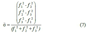
where, f_pf ₂ and f₃represent first, second and third objective functions, respectively.

 

VI. The evaluation of the proposed slngle-Objective Optimization Algorithm

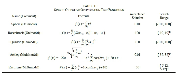
To evaluate the proposed algorithm for single-objective optimization problems, five evaluating functions are utilized. Table I illustrates two required features of these functions: the search range and the acceptance solution value. Among these five functions, all borrowed from the work of Yao et al. [70], three are unimodal and the other two are multimodal. Unimodal functions possess only one optimal answer, while multimodal functions have some local optimal answers in addition to the universal one. To verify the proposed method, the results are compared to four well-known and efficient algorithms, i.e. PSO, ABC, BF and multi-crossover genetic algorithm, in terms of response accuracy and convergence speed. In all the experiments, the population size, the dimensions, and the function value calculation cost are assumed to be 20, 30 and 20><10⁵ respectively, while the objective is to minimize the functions. Therefore, the results of each algorithm are averaged for each of the evaluation functions in 30 runs.

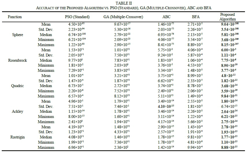
A.Evaluating Accuracy of Results

Accuracy of the proposed algorithm results, through 30 independent runs, has been portrayed in Table II which contains mean, standard deviation, median, minimum, and the maximum optimal responses. As it is illustrated, this algorithm yields a better performance for four evaluation functions, i.e. Sphere, Rosenbrock, Quadric and Rastrigin. For the Ackley, standard deviation calculated by ABC algorithm is superior to others, however, this superiority is negligible in comparison with the proposed algorithm. Moreover, in the remaining categories the proposed algorithm shows better results.

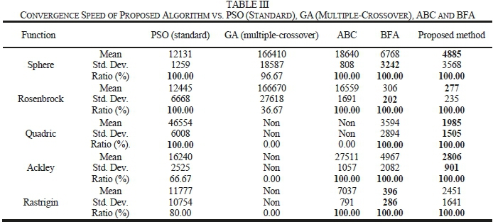
B.Evaluating the Speed of Convergence

Convergence speed which is defined as the required number of calculations for function value so to achieve an acceptable solution plays a vital role in realistic optimization problems. In this section, convergence speed of the proposed algorithm is compared to those of the aforementioned algorithms with regards to evaluation functions presented in Table I. For each algorithm, mean, standard deviation, and convergence speed percentage in 30 independent runs have been calculated for each of the evaluation functions and listed in Table III. As it can be seen, the proposed algorithm surpasses conventional algorithms in terms of convergence speed. The number of achieving an acceptable solution out of 30 times of experiment, also known as convergence percentage, for both of the proposed and the BF algorithms is equal to 100, which means they outweigh other algorithms. For the Rastrigin function, the mean and the standard deviation values resulted from BF algorithm are superior to those of the others. It is noteworthy that for this function, the proposed algorithm offers better solutions than the other three. Furthermore, the deviation values obtained by BF algorithm for Sphere and Rosenbrock functions are more favorable than the other algorithms; however, they are not much different than the same values achieved by the proposed algorithm. As it is evident, the proposed algorithm is superior in the remaining criteria.

 

VII. The Evaluation of the Multi-Objective Proposed Optimization Algorithm

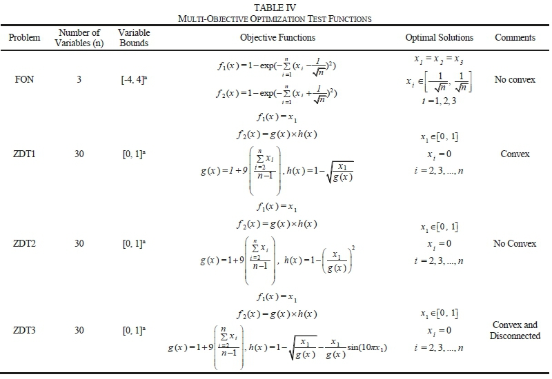
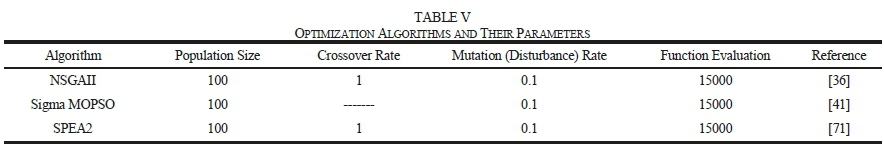
In order to evaluate the proposed hybrid algorithm for multi-objective optimization problems, four renowned multi-objective test functions, listed in Table IV, are employed. The solutions resulted from this algorithm are compared to those of the three other well-known optimization algorithms. Further, the regulation parameters of these three are shown in Table V. To compare the quantitative performance of multi-objective optimization algorithms, three criteria have been regarded.

A. The Metric System of Generational Distance

This metric system is a proper criterion to find the distance between obtained non-dominated solutions and the true Pareto optimal front. This metric system is calculated by using equation (8).

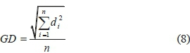
where, n is the number of non-dominated solutions and d_i is the minimum Euclidian distance between member i of non-dominated solutions and the true optimal Pareto front. Indeed, if all members of non-dominated solutions be placed on the Pareto front, then GD =0.

B. The Metric System of Diversity

Evaluates the distribution of non-dominated solutions. It is represented by symbol Δ and computed through equation (9).

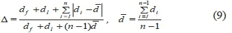
where, d _land d_findicate the Euclidian distances between limited and marginal solutions, respectively. d _lis the Euclidian distance between resulted non-dominated solutions. To obtain the most scattering non-dominated solutions, it is assumed that Δ = 0 .

C. The Metric System of Maximum Spread

This metric system examines the quality of the optimized Pareto front using extreme values of the true and the newly optimized Pareto fronts, and it is calculated as follows:

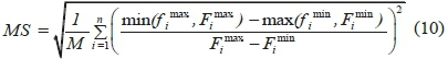
where, M is the number of functions, f_j^minand f_i^maxare the minimum and maximum values of the i^th objective function in the obtained non-dominated solutions. F_i^minand F_i^maxrefer to the minimum and maximum values of i^th objective function of the true Pareto front. Similarly, to have a maximum spread of the non-dominated answers, it should be assumed that MS =1.

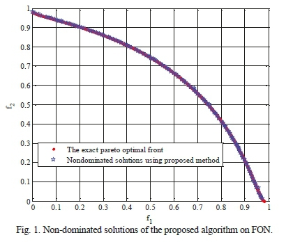
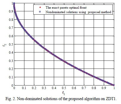
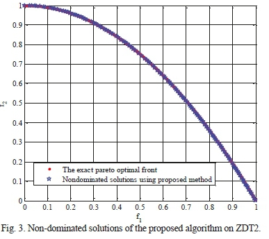
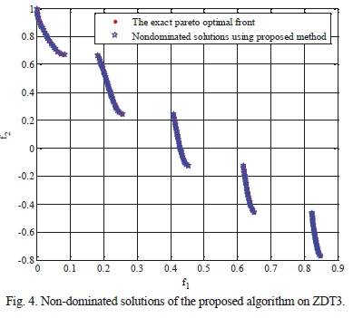
Results and the average values of the aforementioned metrics, obtained from 30 runs of the algorithms on the multi-objective test functions, are shown in Tables VI-IX. Each algorithm's stopping criterion is considered to be 150 repetitions for each run and the population size is taken as 100. In this respect, a set of 500 responses of true Pareto front, uniformly distributed in the space of objective functions, is utilized. As it can be observed, for the multi-objective test functions listed in Table IV, the proposed algorithm yields better responses than other algorithms in terms of all metric systems. For further investigation, the non-dominated solutions obtained by this algorithm are shown in Figs. 1-4 alongside the true optimal Pareto front. As the figures illustrate, Pareto fronts of the proposed algorithm are quite close to the true optimal solutions. In fact, it overlaps the true solutions with high precision.

 

 

 

 

 

 

 

 

VIII. Sliding Mode Control (SMC) and Decoupled Sliding Mode Control (DSMC)

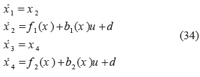
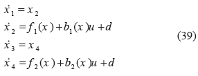
State space equations of a nonlinear fourth-order system is considered to be:

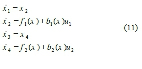
where, x = [x ₁x ₂x ₃x ₄ ]^T is the state vector; f_x, f ₂, b₁ and b₂are nonlinear functions; and u_xand u₂ indicate the control inputs. Further, two sliding surfaces are defined as following:

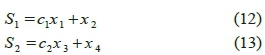
in which, Cj and c₂are the positive constants. According to sliding mode control theory, control laws can be defined as:

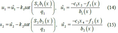
where, k₁and k ₂ are design parameters; q₁and q₂are the widths of boundary layers of sliding surfaces; and u₁and u₂ denote the equivalent- control inputs which are calculated by considering that S and S equal zero. From equation (11). it can be inferred that if u = u = u then only either x ₁ and x ₂ around the sliding surface S ₁, or x ₃ and x ₄ around thesliding surface S ₂ approach zero. In other words, the classic sliding mode control can only control one of these sets: x ₁ and x ₂, or x ₃ and x ₄. However, the true aim is to design a system that can handle both subsystems simultaneously. One way to achieve that goal is using the decoupled sliding mode approach.

This method first divides the system into two subsystems, i.e. A and B. Subsystem A includes x₁ and x₂variables and the sliding surface S ₁, while subsystem B comprises x ₃ and x ₄variables and the sliding surface S ₂. The main purpose of this controller is to direct the state variables in subsystem A towards the sliding surface S₁, which equals zero, so x ₁ and x ₂in turn approach zero exponentially. The second purpose is to reach the sliding surface S ₂ , which also equals zero, by using the state variables of subsystem B. Since the main objective is to stabilize system A, information of system B is considered the secondary data, which has to be transmitted via a mechanism to the primary data. Hence, a new variable called z is defined which conducts this transmission. The sliding surface Si is then transformed as follows:

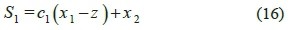
Thus, the main objective changes from x ₁= 0 and x ₂ = 0 to x ₁ = z and x ₂ = 0 , in a way that z is a function of S ₂. Now both primary and secondary objectives are correlated and can be controlled simultaneously, using z which is defined as:

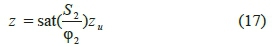
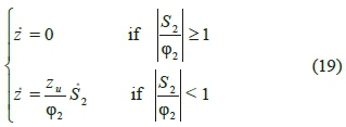
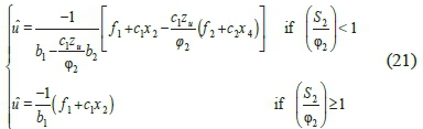
where, φ₂ indicates the width of the boundary layer for S2, and z_urepresents the upper range of z . Since the control input belongs to sliding mode controller of system A, therefore, according to the sliding mode control theory, u = u_jis regarded for the whole system. Moreover, boundary layers of x₁ can be determined by 0 < z_u < 1 and \z\ < z_u. in other words, the maximum absolute value of x₁is always bounded. Thus, z_uis the upper bound of |z|, and also a decreasing signal, since because it is less than 1. The main purpose of equation (16) is to set x ₁ and x ₂ equal to zero, based on the sliding mode control [26]. Resultantly, to control a fourth-order system using sliding mode control the following is obtained:

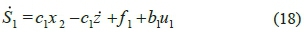
in which,

On the other hand,

it is also possible to determine the control input û by setting equation (18) equal to zero as follows:

With regards to sliding mode theory, a system must be controlled in such circumstances that all the routes lead to the sliding surface. To this end, a discontinuous sentence is added to the equivalent control:

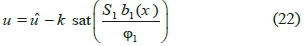
where, k is the design parameter, and φ₁ indicates the width of boundary layer of sliding surface S₁.

 

IX. Decoupled Fuzzy Sliding Mode Control (DFSMC)

The basis of this controller is the same as decoupled sliding mode controller, but with a minor distinction of defining the control coefficients c₁, c ₂, φ₁ and φ₂ through using fuzzy logic. To this end, Singleton fuzzifier, product inference engine and the weighted average defuzzifier are employed to express if-then rules as follows:

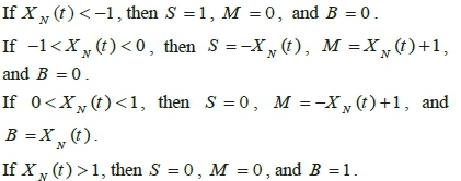
in which, for design coefficients c₁and c₂, XN(t) is equal to normalized values of the state variables x₁and x₃, respectively; whereas, for φ₁ and φ₂, it respectively equals the normalized sliding surfaces S₁ and S ₂. Thus, the fuzzified control coefficients are calculated by followingequations:

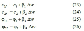
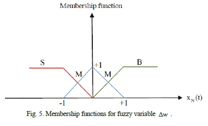
where, c₁f , c_2f, φ_1/and φ_2/are fuzzified control coefficients; β₁, β₂, β₃ and β₄ are in turn some constants utilized as design variables alongside k , z_u, c₁, c₂, φ₁ and φ₂. Further, Δw is calculated as:

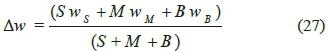
in which, w_S, w_Mand w _Bare equal to 1, 0 and 1, respectively. Fig. 5 displays membership functions for fuzzy variable Δw and fuzzy rules.

 

 

An underactuated system is a plant in which controlled degrees of freedom outnumber the control inputs. In contrast, fully-actuated control systems have only one control input for each degree of freedom. Although underactuated systems outweigh fully-actuated ones in terms of energy saving and production cost reduction, controlling such systems are considerably more complicated due to insufficiency of control inputs. Consider the following dynamic system:

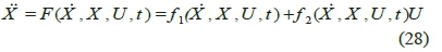
where, X , U and t represent position vector, control input vector and time, respectively. A dynamic system with the above-mentioned equation is fully-actuated if rank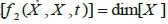, and it is underactuated if rank.

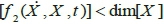The proposed optimal control method is employed and evaluated on three different systems: underactuated inverted pendulum, ball and beam and seesaw, which are all nonlinear, inherently unstable and fourth-order systems.

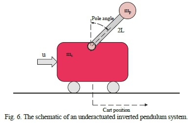
A. Underactuated Inverted Pendulum System

Inverted pendulum constitutes a well-known classic system in dynamics and control engineering. This system comprises a pole attached to a cart moving on a track by the external power u from a DC motor. Fig. 6 illustrates the schematic of an underactuated inverted pendulum system. Dynamic equations of this system are as follows:

 

 

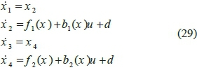
in which,

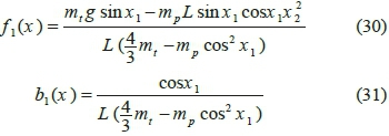
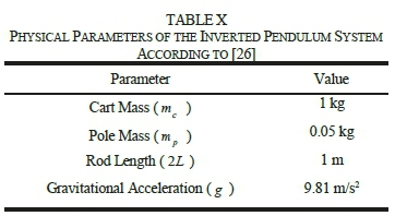
χ=Q is the angle between pole and the vertical axis; χ = θ is the angular velocity of pole relative to the vertical axis; χ₃ = χ is the location of the cart; χ₄ = χis the velocity of the cart; mc is the mass of the cart; m _pis the mass of pole; m_tis the sum of masses of pole and the cart ( m_t = m_c + m_p); L is half of the length of the rod; g is the gravitational acceleration; and d is the absolute value of external disturbances exerted on the system, which does not exceed 0.0873 (|d|< 0.0873). The desirable objective is to stabilize the system around its unstable equilibrium point, i.e. maintaining the pole in vertical position (x _l=θ = 0) and placing the cart at the origin (x ₃= x = 0). The physical parameters of the system are listed in Table X according to Hung & Chung's work [26].

 

 

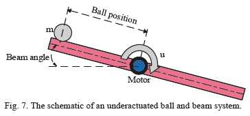
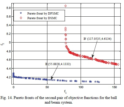
B. Underactuated Ball and Beam System

This system is one the most well-known and prominent experimental models in control systems engineering. Comprehending this system is quite simple and it covers many classical and cutting-edge approaches in respect of stabilization. A metal ball rolls on top of a long beam in this system. The beam, in turn, is mounted on an electrical motor shaft, and can tilt around its central axis by an electrical control signal ( u ). The control objective is to regulate the position of the ball on the beam so that it moves on the beam with a relative acceleration to the beam oscillation. Fig. 7 illustrates the schematic of this system.

 

 

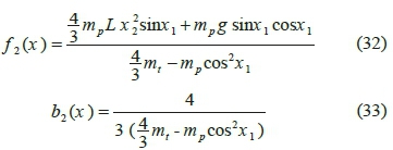
Dynamic equations of this system are as below:

in which,

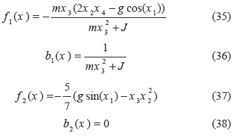
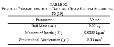
where, x ₁ = θ is the angle between beam and vertical axis; χ₂ = θ denotes the angular velocity of beam related to vertical axis; x₃ = x indicates the position of ball; x₄ =x refers to the ball speed; J is the beam's inertia moment; and, finally, g is the gravitational acceleration. In this system the desirable objective is to keep the beam horizontal, (x ₁ =θ = 0) and the ball at the center of beam (

x₃ = x = 0). The physical parameters of this system are shown in Table XI according to a work done by Mahmoodabadi et al. [10].

 

 

Schematic form of an underactuated seesaw system is demonstrated in Fig. 8. Regarding the basics of physics, if the vertical line along the center of gravity of the inverted wedge does not pass through the fulcrum perpendicularly, then, the inverted wedge will result in a torque and rotate until reaching the stable state. In order to achieve a stable state, this system is equipped with a cart which is free to move on the wedge. With an external force (u ) exerted on the wedge, an opposite torque will be produced, which can lead to stability of the system. Dynamic equations of this system are as below:

 

 

 

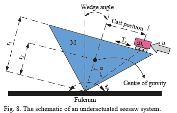
in which;

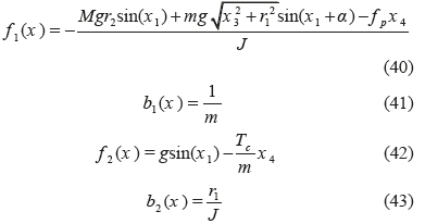
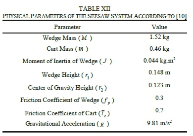
where, x ₁ = θ is the angle between vertical line along the wedge's center of gravity and the perpendicular line from the fulcrum; χ₂=θ is wedge's angular velocity; x₃=x denotes the position of wedge; χ ₄ = χrefers to the velocity of wedge; M and m are respectively the masses of inverted wedge and cart; g , in turn, indicates the gravitational acceleration; while, r₁and r₂respectively represent the heights of inverted wedge its center of gravity (CG). Furthermore, J is the moment of inertia of the inverted wedge; f _pdenotes the rotational friction coefficient of the wedge; T_crepresents the friction coefficient of the cart; and finally, x= tan^_1(x ₃/ r₁) signifies the angle between the line drawn from fulcrum to the cart wheels and the perpendicular line from the fulcrum which also passes through the CG of the wedge. In this system, the ultimate objective is to stabilize the system around its unstable equilibrium point, namely, coincidence of the vertical axis passing through the CG of the wedge with the axis perpendicular to fulcrum (x ₁ =θ = 0), and positioning the wedge at the origin (x ₃ = x = 0). Physical parameters of this system, according to the same in [10], are listed in Table XII.

 

 

XI. Simulation of Underactuated Systems

In this study, the simulation for the above introduced systems along with the control and optimization operation is carried out by MATLAB software. Proper objective functions are defined for each system, and the optimization is performed by using the proposed hybrid algorithm for both DSMC and DFSMC controllers. In all optimization operations, the population size and the number of iterations are considered to be 80 and 100, respectively. Furthermore, during the process, a constraint known as the maximum absolute value of the control force is defined for each system such that designing control coefficients would not cause it to exceed a certain number.

A. Simulation and Results for Underactuated Inverted Pendulum System

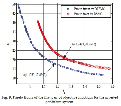
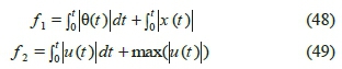
In order to design a multi-objective optimization for the underactuated inverted pendulum system, two pairs of objective functions are utilized. The first is defined as follows:

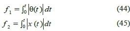
in which, f ₁ indicates the sum of area under the graph of pole angle change, and f ₂ represents the sum of area under graph of cart position change.

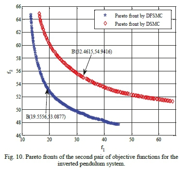
The second pair is introduced as in (46) and (47):

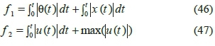
where, f ₁ denotes the total sum of areas under the graphs of pole angle change and sum of areas under the graphs of cart position change, while f ₂ signifies the total sum of area

under the graph of force control and its maximum absolute value. In this system, for both groups of functions, t is considered 20 seconds and the maximum absolute value of control force is equal to 40N. Initial values of the system are as follows:

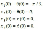
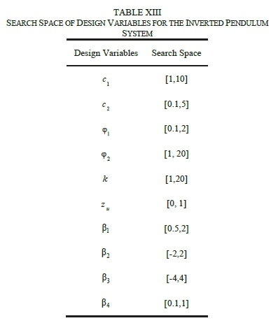
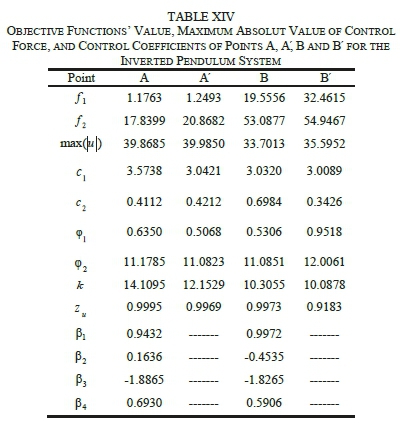
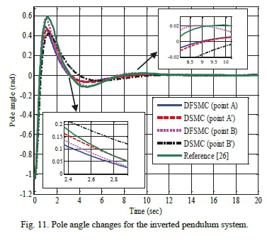
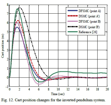
Table XIII shows the search space of design variables for achieving optimal solutions by the proposed algorithm for inverted pendulum system. Figs. 9 and 10 illustrate the comparative Pareto plots resulted from optimization of the two pairs of objective functions. As it can be observed, DFSMC offers superior responses in comparison with the DSMC, in both cases. Table XIV, moreover, displays objective function values, maximum absolute value of control force, and the control coefficients of points A, A, B and B' for both controllers. This table also demonstrates that DFSMC outperforms the DSMC in terms of objective function responses and maximum absolute value of control force. For further validation of the proposed solution, cart position change and pole angle change graphs around the optimal points A, A, B and B' are compared with Hung and Chung's work in which they introduced a decoupled fuzzy sliding mode controller, in conjunction with the fuzzy neural network, to control the inverted pendulum system. As it is evident from Figs. 11 and 12, responses collected from DFSMC surpass those of the mentioned in [26] in respect of control performance around the equilibrium points. Data show that the novel approach successfully causes the cart position and the pole angle to converge to the optimal state in a shorter time.

 

 

 

 

 

 

 

 

 

 

 

 

B. Simulation and Results for the Underactuated Ball and Beam System

To achieve an optimal multi-objective design for the underactuated ball and beam system, two pairs of objective functions are employed as follows: First pair:

Second pair:

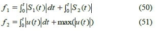
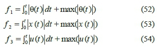
In the first pair, objective function f₁represents the total sum of areas under the graphs of beam angle and sum of areas under the graphs of ball position changes; whereas, objective function f₂indicates the total sum of area under the graph of control force and its maximum absolute value.

In second pair, however, f denotes the total sum of areas under the graphs of siding surfaces S₁and sum of areas under the graphs of siding surfaces S₂, while f₂is the same as in the first pair of functions. In this system t is considered 10 seconds, for both pairs of objective functions, and the maximum absolute value constraint is set equal to 5N. Besides, the initial conditions are defined as follows:

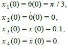
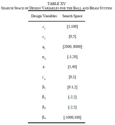
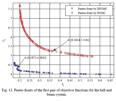
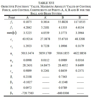
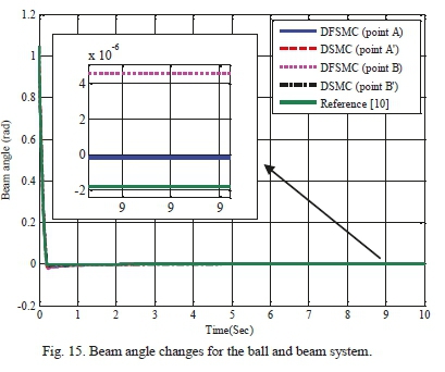
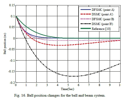
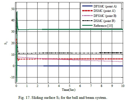
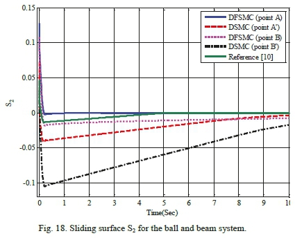
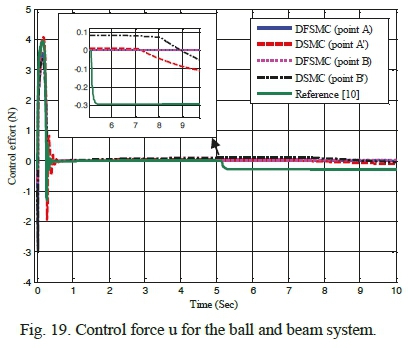
Table XV shows the search space of design variables for achieving optimal solutions through the proposed algorithm for ball and beam system. Figs 13 and 14 represent comparative Pareto plots resulted from optimization of the two pairs of objective functions. As it can be seen, DFSMC controller, in both cases, yields superior responses in comparison with DSMC. Table XVI displays values of objective functions, maximum absolute value of control force, and the control coefficients of points A, A, B and B' for both controllers. This table also demonstrates that DFSMC bring about more optimal responses in terms of objective functions and maximum absolute value of control force compared to the coupled sliding mode controller. For further validation of the proposed solution, control graphs of the optimal points A, A, B and B' are compared with those of the work done by Mahmoodabadi et al. [10], in which, they introduced an optimal DFSMC for underactuated fourth-order nonlinear systems based on the genetic algorithm. As it is apparent from Figs 15-19, solutions of the DFSMC outperform those of DSMC for both pairs of objective functions. In other words, responses of the optimal point A, compared to other selected optimal points and also to those of the mentioned reference [10], can lead system states towards the desirable states more accurately, with less control force and in a shorter period of time.

 

 

 

 

 

 

 

 

 

 

 

 

 

 

 

 

 

 

C. Simulation and Results for the Underactuated Seesaw System

In order to stimulate the underactuated seesaw system and achieve an optimal control, the following three objective functions are defined:

where, f ₁ represents the total sum of area under the graph of wedge angle and its maximum absolute value, f ₂ denotes the total sum of area under the graph of cart position and its maximum absolute value and f ₃ is the total sum of area under the graph of control force and its maximum absolute value. In this system, t is considered 10 seconds and the maximum absolute value of control force is equal to 10 N. Furthermore, the initial conditions in this system are set as follows:

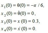
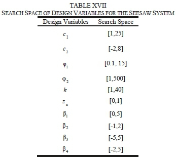
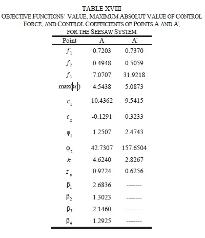
Table XVII shows the search space of design variables for achieving optimal solutions through proposed algorithm for the seesaw system. Fig. 20 displays the Pareto front resulted from optimization implementation of two controllers, i.e. decoupled sliding mode and the decoupled fuzzy sliding mode, based on the proposed optimization algorithm. According to the figure, optimal solutions obtained from the three-objective optimization of DFSMC are superior to those of DSMC in terms of metric systems of generational distance, diversity and maximum spread. Moreover, Table XVIII demonstrates values of objective functions, maximum absolute value of control force, and the control coefficients of points A and A' for both controllers. This Table also denotes that decoupled fuzzy sliding mode controller has achieved more optimal responses regarding three aforementioned objective functions and the maximum absolute value of control force. Additionally, for validation and further examination of the two controllers, control graphs of the selected optimal points A and A' are compared with those of the work of Mahmoodabadi et al. [10]. As it is evident from Figs. 21-25, responses obtained from the proposed algorithm in the present study show a superiority to those from decoupled sliding mode controller and those of the mentioned in [10].

 

 

 

 

 

 

 

 

 

 

 

 

 

 

 

 

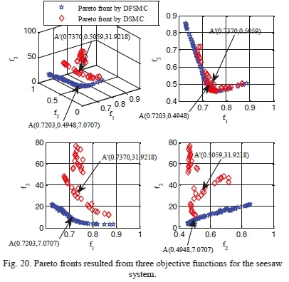
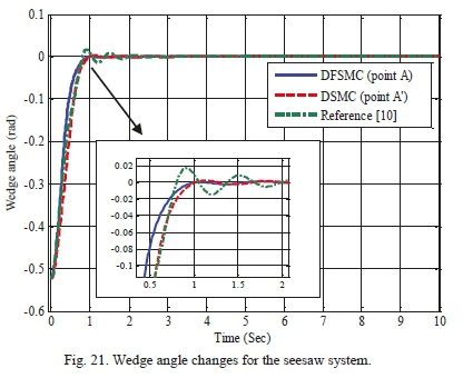
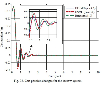
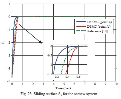
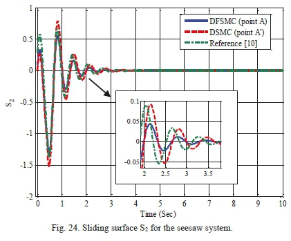
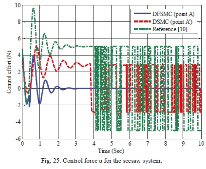
These Figures reveal that the proposed algorithm can overlap optimal states more accurately and with less control force. Looking at the graphs of the control force resulted from DSMC and the mentioned in [10] proves that there exist undesirable effects of chattering phenomenon (Fig 25); whereas the DFSMC does not bring about such unwanted effects and can cause the control force to converge to zero in less than 3 seconds.

This paper proposes an optimal multi-objective decoupled fuzzy sliding mode control technique, based on a robust hybrid optimization algorithm, to control and stabilize underactuated nonlinear coupled systems. This approach is a general and desirable design technique used to achieve control objectives for some sorts of nonlinear systems. The underlying idea of this proposed optimization algorithm is that the artificial bee colony (ABC) and the bacterial foraging (BF) algorithms be optimally combined.

This technique, moreover, requires two steps for implementation. The first is to design a decoupled fuzzy sliding mode control; and the second comprises employing the proposed hybrid algorithm to search within the determined space of design variables and achieve the best responses in form of an optimal Pareto front. The simulation and results on three nonlinear systems, i.e. inverted pendulum, ball and beam and seesaw, show that the proposed technique is able to achieve an accurate control together with stable operation of those systems around their equilibrium Points.

 

References

[1] J. J. E. Slotine, and W. Li, Applied Nonlinear Control, New Jersey, United States of America: Prentice-Hall, Englewood Cliffs, 1991, pp. 276-310.

[2] M. W. McConley, B. D. Appleby, M. A. Dahleh, and E. Feron, "A computationally efficient lyapunov-based scheduling procedure for control of nonlinear systems with stability guarantees," IEEE Transactions on Automatic Control, vol. 45, no. 1, pp. 33-49, Jan. 2000. DoI: 10.1109/9.827354.         [ Links ]

[3] C. Belta, and L. C. G. J. M. Habets, "Controlling a class of nonlinear systems on rectangles," IEEE Transaction on Automatic Control, vol. 51. no. 11, pp. 1749-1759, Nov. 2006. DOI: 10.1109/TAC.2006.884957.         [ Links ]

[4] Y. Niu, D. W. C. Ho, and X. Wang, "Robust H„ control for nonlinear stochastic systems: a sliding-mode approach," IEEE Transactions on Automatic Control, vol. 53, no. 7, pp. 1695-1701, Aug. 2008. DOI: 10.1109/TAC.2008.929376.         [ Links ]

[5] S. Elloum, and N. Benhadj Braiek, "On feedback control techniques of nonlinear analytic systems," Journal of Applied Research and Technology, vol. 12, no. 13, pp. 500-513, Jun. 2014. Accessed on: Mar., 06, 2015, DOI: 10.1016/S1665-6423(14)71630-X, [Online].         [ Links ]

[6] Y. J. Liu, C. L. Philip Chen, G. X. Wen, and S. Tong, "Adaptive neural output feedback tracking control for a class of uncertain discrete-time nonlinear systems," IEEE Transactions on Neural Networks, vol. 22, no. 7, pp. 1162-1167, Jul. 2011. DOI: 10.1109/TNN.2011.2146788.         [ Links ]

[7] J. Kang, W. Meng, A. Abraham, and H. Liu, "An adaptive PID neural network for complex nonlinear system control," Neurocomputing, vol. 135, pp. 79-85, Jul. 2014. Accessed on: Jan., 04, 2014, DOI: 10.1016/j.neucom.2013.03.065, [Online].         [ Links ]

[8] S. Tong, L. Zhang, and Y. Li, "Observed-based adaptive fuzzy decentralized tracking control for switched uncertain nonlinear large-scale systems with dead zones," IEEE Transactions on Systems, Man, and Cybernetics: Systems, vol. 46, no. 1, pp. 37-47, Jan. 2016. DOI: 10.1109/TSMC.2015.2426131.         [ Links ]

[9] Q. Zhang, D. Zhao, and D. Wang, "Event-based robust control for uncertain nonlinear systems using adaptive dynamic programming," IEEE Transactions on Neural Networks and Learning Systems, vol. 29, no. 1, pp. 37-50, Jan. 2018. DOI: 10.1109/TNNLS.2016.2614002.         [ Links ]

[10] M. J. Mahmoodabadi, A. Bagheri, N. Nariman-Zadeh, A. Jamali, and R. Abedzadeh Maafi, "Pareto design of decoupled sliding-mode controllers for nonlinear systems based on a multiobjective genetic algorithm," Journal of Applied Mathematics, vol. 2012, Article ID 639014, 22 pages, Apr. 2012. DOI:10.1155/2012/639014.         [ Links ]

[11] F. Yorgancioglu, and H. Komurcugil, "Decoupled sliding-mode controller based on time-varying sliding surfaces for fourth-order systems," Expert Systems with Applications, vol. 37, no. 10, pp. 6764-6774, Oct. 2010. Accessed on: Mar., 25, 2010, DOI: 10.1016/j.eswa.2010.03.049, [Online].         [ Links ]

[12] S. G. Tzafestas, and G. G. Rigatos, "Design and stability analysis of a new sliding-mode fuzzy logic controller of reduced complexity," Machine Intelligence & Robotic Control, vol. 1, no. 1, pp. 27-41, Jan. 1999. [Online]. Available: https://www.academia.edu/11969153/Design_and_stability_analysis_of_a_new_sliding-mode_fuzzy_logic_controller_of_reduced_complexity.         [ Links ]

[13] M. Roopaei, and M. Zolghadri Jahromi, "Chattering-free fuzzy sliding mode control in MIMO uncertain systems," Nonlinear Analysis: Theory, Methods & Applications, vol. 71, no. 10, pp. 4430-4437, Nov. 2009. Accessed on: Mar., 09, 2009, DOI: 10.1016/j.na.2009.02.132, [Online].         [ Links ]

[14] L. A. Zadeh, "Fuzzy algorithms," Information and Control, vol. 12, no. 2, pp. 94-102, Feb. 1968. Accessed on: Nov., 29, 2004, DOI: 10.1016/S0019-9958(68)90211-8, [Online].         [ Links ]

[15] L. A. Zadeh, "Outline of a new approach to the analysis of complex systems and decision processes," IEEE Transactions on Systems, Man and Cybernetics, vol. SMC-3, no. 1, pp. 28-44, Jan. 1973. DOI: 10.1109/TSMC.1973.5408575.         [ Links ]

[16] B. S. Chen, C. S. Tseng, and H. J. Uang, "Robustness design of nonlinear dynamic systems via fuzzy linear control," IEEE Transactions on Fuzzy Systems, vol. 7, no. 5, pp. 571-585, Oct. 1999. DOI: 10.1109/91.797980.         [ Links ]

[17] A. B. Sharkawy, H. El-Awady, and K. A. F. Moustafa, "Stable fuzzy control for a class of nonlinear systems," Transactions of the Institute of Measurement and Control, vol. 25, no. 3, pp. 265-278, Aug. 2003. DOI: 10.1191/0142331203tm086oa.         [ Links ]

[18] C. S. Tseng, B. S. Chen, and Y. F. Li, "Robust fuzzy observer-based fuzzy control design for nonlinear systems with persistent bounded disturbances: A novel decoupled approach," Fuzzy Sets and Systems, vol. 160, no. 19, pp. 2824-2843, Oct. 2009. Accessed on: Feb., 21, 2009, DOI: 10.1016/j.fss.2009.02.006, [Online].         [ Links ]

[19] S. Tong, C. Liu, and Y. Li, "Fuzzy-adaptive decentralized output-feedback control for large-scale nonlinear systems with dynamical uncertainties," IEEE Transactions on Fuzzy Systems, vol. 18, no. 5, pp. 845861, Oct. 2010. DOI: 10.1109/TFUZZ.2010.2050326.         [ Links ]

[20] P. Li, and F. J. Jin, "Adaptive fuzzy control for unknown nonlinear systems with perturbed dead-zone inputs," Acta Automatica Sinica, vol. 36, no. 4, pp. 573-579, Apr. 2010. Accessed on: Apr., 18, 2010, DOI: 10.1016/S1874-1029(09)60024-0, [Online].         [ Links ]

[21] T. S. Wu, M. Karkoub, C. T. Chen, W. S. Yu, M. G. Her, and J. Y. Su, "Robust tracking design based on adaptive fuzzy control of uncertain nonlinear MIMO systems with time delayed states," International Journal of Control, Automation and Systems, vol. 11, no. 6, pp. 1300-1313, Nov. 2013. Accessed on: Nov., 29, 2013, DOI: 10.1007/s12555-012-0543-x, [Online].         [ Links ]

[22] Y. J. Liu, and S. Tong, "Adaptive fuzzy control for a class of unknown nonlinear dynamical systems," Fuzzy Sets and Systems, vol. 236, pp. 49-70, Mar. 2015. Accessed on: Aug., 26, 2014, DOI: 10.1016/j.fss.2014.08.008, [Online].         [ Links ]

[23] J. Qiu, S. X. Ding, H. Gao, and S. Yin, "Fuzzy-model-based reliable static output feedback H„ control of nonlinear hyperbolic PDE systems," IEEE Transactions on Fuzzy Systems, vol. 24, no. 2, pp. 388-400, Apr. 2016. DOI: 10.1109/TFUZZ.2015.2457934.         [ Links ]

[24] B. Yoo, and W. Ham, "Adaptive fuzzy sliding mode control of nonlinear system," IEEE Transactions on Fuzzy Systems, vol. 6, no. 2, pp. 315-321, May 1998. DOI: 10.1109/91.669032.         [ Links ]

[25] H. X. Li, and S. Tong, "A hybrid adaptive fuzzy control for a class of nonlinear MIMO systems," IEEE Transactions on Fuzzy Systems, vol. 11, no. 1, pp. 24-34, Feb. 2003. DOI: 10.1109/TFUZZ.2002.806314.         [ Links ]

[26] L. C. Hung, and H. Y. Chung, "Decoupled sliding-mode with fuzzy-neural network controller for nonlinear systems," International Journal of Approximate Reasoning, vol. 46, no. 1, pp. 74-97, Sep. 2007. Accessed on: Oct., 04, 2006, DOI: 10.1016/j.ijar.2006.08.002, [Online].         [ Links ]

[27] H. F. Ho, Y. K. Wong, and A. B. Rad, "Adaptive fuzzy sliding mode control with chattering elimination for nonlinear SISO systems," Simulation Modelling Practice and Theory, vol. 17, no. 7, pp. 1199-1210, Aug. 2009. Accessed on: Apr., 21, 2009, DOI: 10.1016/j.simpat.2009.04.004, [Online].         [ Links ]

[28] Y. H. Chang, C. W. Chang, C. W. Tao, H. W. Lin, and J. S. Taur, "Fuzzy sliding-mode control for ball and beam system with fuzzy ant colony optimization," Expert Systems with Applications, vol. 39, no. 3, pp. 36243633, Feb. 2012. Accessed on: Sep., 29, 2011, DOI: 10.1016/j.eswa.2011.09.052, [Online].         [ Links ]

[29] N. Bouarroudj, D. Boukhetala, and F. Boudjema, "A hybrid fuzzy fractional order PID sliding-mode controller design using PSO algorithm for interconnected nonlinear," Control Engineering and Applied Informatics, vol. 17, no. 1, pp. 41-51, 2015.         [ Links ]

[30] B. A. Elsayed, M. A. Hassan, and S. Mekhilef, "Fuzzy swinging-up with sliding mode control for third order cart-inverted pendulum system," International Journal of Control, Automation and Systems, vol. 13, no. 1, pp. 238-248, Feb. 2015. Accessed on: Dec., 18, 2014, DOI: 10.1007/s12555-014-0033-4, [Online].         [ Links ]

[31] M. J. Mahmoodabadi, R. Abedzadeh Maafi, and M. Taherkhorsandi, "An optimal adaptive robust PID controller subject to fuzzy rules and sliding modes for MIMO uncertain chaotic systems," Applied Soft Computing, vol. 52, pp. 1191-1199, Mar. 2017. Accessed on: Sep., 07, 2016, DOI: 10.1016/j.asoc.2016.09.007, [Online].         [ Links ]

[32] Y. Wang, H. Shen, H. R. Karimi, and D. Duan, "Dissipativity-based fuzzy integral sliding mode control of continuous-time T-S fuzzy systems," IEEE Transactions on Fuzzy Systems, vol. 26, no. 3. pp. 1164-1176, Jun. 2018. DOI: 10.1109/TFUZZ.2017.2710952.         [ Links ]

[33] J. Nocedal, and S. J. Wright, Numerical Optimization, 2nd ed., New York City, New York, United States of America: Springer, 2006, pp. 193 -219. [Online]. Available: https://link.springer.com/book/10.1007/978-0-387-40065-5.

[34] M. Mitchell, An Introduction to Genetic Algorithms, Cambridge, Massachusetts, United States of America: MIT Press, 1999, 209 pages.

[35] K. Deb, and H. G. Beyer, "Self-adaptive genetic algorithms with simulated binary crossover," Evolutionary Computation, vol. 9, no. 2, pp. 197-221, Jun. 2001. DOI: 10.1162/106365601750190406.         [ Links ]

[36] K. Deb, A. Pratap, S. Agarwal, and T. Meyarivan, "A fast and elitist multiobjective genetic algorithm: NSGA-II," IEEE Transactions on Evolutionary Computation, vol. 6, no. 2, pp. 182-197, Apr. 2002. DOI: 10.1109/4235.996017.         [ Links ]

[37] S. Elaoud, J. Teghem, and T. Loukil, "Multiple crossover genetic algorithm for the multiobjective traveling salesman problem," Electronic Notes in Discrete Mathematics, vol. 36, pp. 939-946, Aug. 2010. Accessed on: Jul., 17, 2010, DOI: 10.1016/j.endm.2010.05.119, [Online].         [ Links ]

[38] Q. Long, C. Wu, T. Huang, and X. Wang, "A genetic algorithm for unconstrained multi-objective optimization," Swarm and Evolutionary Computation, vol. 22, pp. 1-14, Jun. 2015. Accessed on: Jan., 27, 2015, DOI: 10.1016/j.swevo.2015.01.002, [Online].         [ Links ]

[39] J. Kennedy, and R. Eberhart. (1995, 27 Nov.-1 Dec.). Particle swarm optimization. Presented at Proceedings of ICNN'95-International Conference on Neural Networks. Perth, WA, Australia. [Online]. Available: https://ieeexplore.ieee.org/document/488968.

[40] P. J. Angeline. (1998, 4-9 May).Using selection to improve particle swarm optimization. Presented at 1998 IEEE International Conference on Evolutionary Computation Proceedings. IEEE World Congress on Computational Intelligence (Cat. No.98TH8360). Anchorage, AK, USA. [Online]. Available: https://ieeexplore.ieee.org/abstract/document/699327.

[41] S. Mostaghim, and J. Teich. (2003, 26 Apr.). Strategies for finding good local guides in multi-objective particle swarm optimization (MOPSO). Presented at Proceedings of the 2003 IEEE Swarm Intelligence Symposium. SIS'03 (Cat. No.03EX706). Indianapolis, IN, USA. [Online]. Available: https://ieeexplore.ieee.org/document/1202243.

[42] F. Marini, and B. Walczak, "Partical swarm optimization (PSO). a tutorial," Chemometrics and Intelligent Laboratory Systems, vol. 149, pp. 153-165, Dec. 2015. Accessed on: Sep., 12, 2015, DOI: 10.1016/j.chemolab.2015.08.020, [Online].         [ Links ]

[43] W. Ye, W. Feng, and S. Fan, "A novel multi-swarm particle swarm optimization with dynamical learning strategy," Applied Soft Computing, vol. 61, pp. 832-843, Dec. 2017. Accessed on: Sep., 01, 2017, DOI: 10.1016/j.asoc.2017.08.051, [Online].         [ Links ]

[44] D. Karaboga, "An idea based on honey bee swarm for numerical optimization,", Technical Report, Kayseri, Turkey, TR06, Oct. 2005. [Online]. Available: https://pdfs.semanticscholar.org/015d/f4d97ed1f541752842c49d12e429a785460b.pdf.

[45] D. Karaboga, and B. Basturk, "A powerful and efficient algorithm for numerical function optimization: artificial bee colony (ABC) algorithm," Journal of Global Optimization, vol. 39, no. 3, pp. 459-471, Nov. 2007. Accessed on: Apr., 13, 2007, DOI: 10.1007/s10898-007-9149-x, [Online].         [ Links ]

[46] F. Kang, J. Li, and Z. Ma, "Rosenbrock artificial bee colony algorithm for accurate global optimization of numerical functions," Information Sciences, vol. 181, no. 16, pp. 3508-3531, Aug. 2011. Accessed on: Apr., 21, 2011, DOI: 10.1016/j.ins.2011.04.024, [Online].         [ Links ]

[47] F. J. Rodriguez, M. Lozano, C. García-Martínez, and J. D. González-Barrera, "An artificial bee colony algorithm for the maximally diverse grouping problem," Information Sciences, vol. 230, pp. 183-196, May 2013. Accessed on: Jan., 08, 2013, DOI: 10.1016/j.ins.2012.12.020, [Online].         [ Links ]

[48] J. Li, Q. Pan, and P. Duan, "An improved artificial bee colony algorithm for solving hybrid flexible flowshop with dynamic operation skipping," IEEE Transactions on Cybernetics, vol. 46, no. 6, pp. 1311-1324, Jun. 2016. DOI: 10.1109/TCYB.2015.2444383.         [ Links ]

[49] F. Chengli, F. Qiang, L. Guangzheng, and X. Qinghua, "Hybrid artificial bee colony algorithm with variable neighborhood search and memory mechanism," Journal of Systems Engineering and Electronics, vol. 29, no. 2, pp. 405-414, Apr. 2018. DOI: 10.21629/JSEE.2018.02.20.         [ Links ]

[50] J. Yang, Q. Jiang, L. Wang, S. Liu, Y. D. Zhang, W. Li, and B. Wang, An adaptive encoding learning for artificial bee colony algorithms," Journal of Computational Science, vol. 30, pp. 11-27, Jan. 2019. Accessed on: Nov., 10, 2018, DOI: doi.org/10.1016/j.jocs.2018.11.001, [Online].         [ Links ]

[51] K. M. Passino, "Biomimicry of bacterial foraging for distributed optimization and control," IEEE Control Systems Magazine, vol. 22, no. 3, pp. 52-67, Jun. 2002. DOI: 10.1109/MCS.2002.1004010.         [ Links ]

[52] Y. Liu, and K. M. Passino, "Biomimicry of social foraging bacteria for distributed optimization: models, principles, and emergent behaviors," Journal of Optimization Theory and Applications, vol. 115, no. 3, pp. 603628, Dec. 2002. DOI: 10.1023/A:1021207331209.         [ Links ]

[53] N. Amjady, H. Fatemi, and H. Zareipour, "Solution of optimal power flow subject to security constraints by a new improved bacterial foraging method," IEEE Transactions on Power Systems, vol. 27, no. 3, pp. 13111323, Aug. 2012. DOI: 10.1109/TPWRS.2011.2175455.         [ Links ]

[54] X. Lv, H. Chen, Q. Zhang, X. Li, H. Huang, and G. Wang, "An improved bacterial-foraging optimization-based machine learning framework for predicting the severity of somatization disorder," Algorithms, vol. 11, no. 2, 18 pages, Feb. 2018. DOI: 10.3390/a11020017.         [ Links ]

[55] S. Kirkpatrick, C. D. Gelatt Jr., and M. P. Vecchi, "Optimization by simulated annealing," Science, vol. 220, no. 4598, pp. 671-680, May 1983. DOI: 10.1126/science.220.4598.671.         [ Links ]

[56] G. Gong, Y. Liu, and M. Qian, "An adaptive simulated annealing algorithm," Stochastic Processes and their Applications, vol. 94, no. 1, pp. 95-103, Jul. 2001. Accessed on: May, 23, 2001, DOI: 10.1016/S0304-4149(01)00082-5, [Online].         [ Links ]

[57] X. Geng, Z. Chen, W. Yang, D. Shi, and K. Zhao, "Solving the traveling salesman problem based on an adaptive simulated annealing algorithm with greedy search," Applied Soft Computing, vol. 11, no. 4, pp. 3680-3689, Jun. 2011. Accessed on: Feb., 05, 2011, DOI: 10.1016/j.asoc.2011.01.039, [Online].         [ Links ]

[58] L. Cheng, L. Han, X. Zeng, Y. Bian, and H. Yan, "Adaptive cockroach colony optimization for rod-like robot navigation," Journal of Bionic Engineering, vol. 12, no. 2, pp. 324-337, Apr. 2015. Accessed on: Apr., 19, 2015, DOI: 10.1016/S1672-6529(14)60125-6, [Online].         [ Links ]

[59] L. Cheng, L. Han, X. Zeng, and Y. Bian, "A new cockroach colony optimization algorithm for global numerical optimization," Chinese Journal ofElectronics, vol. 26, no. 1, pp. 73-79, Jan. 2017. DOI: 10.1049/cje.2016.06.030.         [ Links ]

[60] C. F. Juang, "A hybrid of genetic algorithm and particle swarm optimization for recurrent network design," IEEE Transactions on Systems, Man, and Cybernetics, Part B, Cybernetics, vol. 34, no. 2, pp. 997-1006, Apr. 2004. DOI: 10.1109/TSMCB.2003.818557.         [ Links ]

[61] Y. Wang, Z. Cai, G. Guo, and Y. Zhou, "Multiobjective optimization and hybrid evolutionary algorithm to solve constrained optimization problems," IEEE Transactions on Systems, Man, and Cybernetics, Part B (Cybernetics), vol. 37, no. 3, pp. 560-575, Jun. 2007. DOI: 10.1109/TSMCB.2006.886164.         [ Links ]

[62] D. H. Kim, A. Abraham, and J. H. Cho, "A hybrid genetic algorithm and bacterial foraging approach for global optimization," Information Sciences, vol. 177, no. 18, pp. 3918-3937, Sep. 2007. Accessed on: Apr., 11, 2007, DOI: 10.1016/j.ins.2007.04.002, [Online].         [ Links ]

[63] T. Niknam, B. Amiri, J. Olamaei, and A. Arefi, "An efficient hybrid evolutionary optimization algorithm based on PSO and SA for clustering," Journal of Zhejiang University-SCIENCEA, vol. 10, no., 4, pp. 512-519, Apr. 2009. Accessed on: Apr., 01, 2009, DOI: 10.1631/jzus.A08201, [Online].         [ Links ]

[64] S. Li, M. Tan, I. W. Tsang, and J. T. Y. Kwok, "A hybrid PSO-BFGS strategy for global optimization of multimodal functions," IEEE Transactions on Systems, Man, and Cybernetics, Part B (Cybernetics), vol. 41, no. 4, pp. 1003-1014, Aug. 2011. DOI: 10.1109/TSMCB.2010.2103055.         [ Links ]

[65] M. J. Mahmoodabadi, M. Taherkhorsandi, R. Abedzadeh Maafi, and K. K. Castillo-Villar, "A novel multi objective optimisation algorithm: artificial bee colony in conjunction with bacterial foraging," International Journal of Intelligent Engineering Informatics, vol. 3, no. 4, pp. 369-386, Nov. 2015. Accessed on: Nov., 13, 2015, DOI: 10.1504/IJIEI.2015.073088, [Online].         [ Links ]

[66] Z. Li, W. Wang, Y. Yan, and Z. Li, "PS-ABC: A hybrid algorithm based on particle swarm and artificial bee colony for high-dimensional optimization problems," Expert Systems with Applications, vol. 42, no. 22, pp. 8881-8895, Dec. 2015. Accessed on: Jul., 26, 2015, DOI: 10.1016/j.eswa.2015.07.043, [Online].         [ Links ]

[67] P. Shunmugapriya, and S. Kanmani, "A hybrid algorithm using ant bee colony optimization for feature selection and classification (AC-ABC Hybrid)," Swarm and Evolutionary Computation, vol. 36, pp. 27-36, Oct. 2017. Accessed on: Apr., 11, 2017, DOI: 10.1016/j.swevo.2017.04.002, [Online].         [ Links ]

[68] D. E. Goldberg, Genetic Algorithms in Search, Optimization and Machine Learning, Boston, Massachusetts, United States of America: Addison-Wesley Longman Publishing Co., Inc., 1989, 372 pages.

[69] A. Ravindran, K. M. Ragsdell, and G. V. Reklaitis, Engineering Optimization: Methods and Applications, 2nd ed., Hoboken, New Jersey, United States of America: John Wiley & Sons, Inc., 2006, 688 pages. [Online]. Available: https://epdf.pub/engineering-optimization-methods-and-applications.html.

[70] X. Yao, Y. Liu, and G. Lin, "Evolutionary programming made faster," IEEE Transactions on Evolutionary Computation, vol. 3, no. 2, pp. 82-102, Jul. 1999. DOI: 10.1109/4235.771163.         [ Links ]

[71] E. Zitzler, M. Laumanns, and L. Thiele, "SPEA2: improving the strength Pareto evolutionary algorithm for multiobjective optimization," Swiss Federal Institute of Technology (ETH), Zurich, Switzerland, TIK-Rep. 103, May. 2001. [Online]. Available: https://pdfs.semanticscholar.org/6672/8d01f9ebd0446ab346a855a44d2b13

 

 

 

M. J. Mahmoodabadi received his B.S. and M.S. degrees in Mechanical Engineering from Shahid Bahonar University of Kerman, Iran, in 2005 and 2007, respectively. He received his Ph.D. degree in Mechanical Engineering from the University of Guilan, Rasht, Iran in 2012.
He worked for two years in the Iranian Textile Industries. During his research, he was a scholar visitor with Robotics and Mechatronics Group, University of Twente, Enchede, the Netherlands for 6 months. Now, he is an assistant professor of Mechanical Engineering at Sirjan University of Technology, Sirjan, Iran. His research interests include optimization algorithms, non-linear and robust control, and computational methods. Corresponding author of this paper.

 

 

R. Abedzadeh Maafi was born in Rasht, Iran, 1986. He received his B.S. and M.S. degrees in Mechanical Engineering from Islamic Azad University, Iran in 2008 and 2012 respectively. Now, he is a Ph.D. student in Mechanical Engineering at the Science and Research Branch of Islamic Azad University, Tehran, Iran. He has been a member of Guilan Construction Engineering Organization and an adjunct lecturer at University of Applied Science and Technology since 2012. His research interests include optimization algorithms, nonlinear and robust control, optimal control, robotics, and computational methods.

 

 

S. Etemadi Haghighi received his B.S. degree in Mechanical engineering from Ferdowsi University of Mashad, Mashad, Iran in 2000. He also received his M.S. and Ph.D. degrees in Mechanical engineering from Sharif University of Technology, Tehran, Iran in 2003 and 2011, respectively. He is currently assistant professor of Department of Mechanical Engineering at Science and Research Branch, Islamic Azad University, Tehran, Iran. His studies are in the field of nonlinear vibration and control and he is interested in swarm robotics and flapping wing robots.

 

 

A. Moradi received his B.S. degree in Mechanical Engineering from the University of Guilan, Iran in 2011 and his M.S. in Mechanical Engineering from Islamic Azad University, Iran in 2013. He has been an adjunct lecturer at University of Applied Science and Technology since 2014 and a member of Guilan Construction Engineering Organization. His research interests include optimal and robust control, optimization algorithms, and optimization numerical approaches.