ARTICLES

 

Rope-Weaver's Principles: Towards More Effective Learning

 

 

R.C. Aylward^I; B.J. van Wyk^II; Y Hamam^III

^IMember, IEEE
^IIMember, IEEE
^IIILife Senior Member IEEE

 

 

---

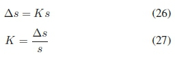
ABSTRACT

This paper introduces a new methodology to assist teaching and learning in a time-constrained environment at the hand of two time-on-task examples. These examples are from the field of Electrical Engineering studies with a focus on first-year studies and an advanced software design course taught at the Tshwane University of Technology in South Africa. In an endeavour to understand the timing model of the human brain to master and assimilate new information, a study was conducted to determine some of the parameters that could possibly have an influence on the timing model and how the brain perceives new information. From this study the Rope-Weaver's Principles were derived and are built on three well-known theories, comparative judgment, the Guttman scale and the learning curve, integrated into the new methodology. The Rope-Weaver's Principles are presented as an abstraction of the mathematical principles and the measures that underpin this study. The research was done from a participant-observer perspective with design research as central methodology. The research methodology involved a longitudinal study employing mixed-methods research. The results led to the observation of a toe or plateau in the infancy of the learning curve. The observed plateau has a direct influence on the order and time frame of the introduction of new study material in a formal educational programme. The results were found to adhere to the Weber-Fechner Law. This relates to other studies on animals, suggesting that the way the brain perceives stimuli or assimilate knowledge is hard-wired throughout the animal kingdom although the brain structures vary widely. It is proposed that Rope-Weaver's Principles, complementary to the current pool of teaching and learning theories, lead to a better mastery of the learning material or skills, moving persons under instruction from rule based training - behaviourism, to maxim integration - constructivism.

Index Terms: Analytic hierarchy network, engineering education, failure modeling, just noticeable difference, learning curves, learning strategies.

---

 

 

I. INTRODUCTION

HAVING spent a quarter of a century committed to tertiary education in the field of engineering studies, at an University of Technology (UoT) in South Africa, and seeing scores of students failing year after year left questions on teaching methodologies. How is it that with lecturers having years' of experience students were still failing? Have the lecturers lost the plot or are they missing something essential? This led to a study on what transpires in the mind of a person under training, which in turn led to following questions: How does one assimilate new knowledge and acquire new skills? How should one adopt new teaching methods or change current teaching methods to facilitate better learning? What is the relation between students' knowledge and skill at the start of the course to that what is mastered or required at the end of the course?

To broaden the scope of the problem the following perspectives are given. There has been a major shift by the South African Department of Education towards Outcomes Based Education (OBE) as opposed to Content Based Education (CBE) in post-millennium curriculum design [8]. Most of the current student cohort in tertiary education passed through this new OBE school of thought and entered the tertiary educational systems in the past 5 years. The objectives of OBE per se are not at fault, but the implementation thereof has left two major shortfalls. First and foremost, the outcomes are focused on delivering young adults ready to contribute to the broader needs of society. This meant expanding the previous curriculum by adding the required material into the new study programmes. As the basic education programme still only spanned a 12 year period the focus shifted to incorporate the new materials. This resulted in a more rounded programme on paper, however, in practice it resulted in less rigorous mathematics and science programmes not producing enough candidates at required level for tertiary studies. Secondly, the novel objectives of self-paced learning and the aim of no student being left behind also fall short of the intended OBE objectives. In a time constrained programme, 12 years for basic education and 4 years tertiary education for a first degree, it is impractical as it leaves the learners underprepared for tertiary studies in engineering and science or industry at large [3].

In Fig. 1 [4] the knowledge levels for mathematics and science levels are shown where the exit levels for the 12 year basic education system for pre-millennium are indicated by Pr2 and those for post-millennium by Po2. Pr1 is the level for learners entering into the 12 year basic education system that precedes the tertiary system shown here. According to the 20 year comparative report of the Trends in International Mathematics and Science Study (TIMMS) the levels for Pr2 and Po2 are quite varied amongst nations [22]. The case shown in Fig. 1 relates to nations showing a decline in mathematics and science scores since 1995, including first world countries like Norway and Sweden. South Africa also falls into this category [25] [32]. The graph is shown for illustrative purposes only and uses relative measures in support of the observations discussed in the text.

 

 

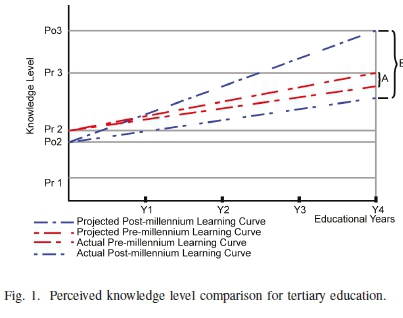
Further support for the Pr2 - Po2 observation can be found in the Centre for Development and Enterprise (CDE) report [6]. It was reported that approximately 10% of candidates passed mathematics, 58 081 candidates, and 6% passed sciences, 33 734 candidates, from a total of 561 477 candidates. Assuming all candidates pursued tertiary education and distributing them equally amongst the 26 South African Universities only, results in only 1300 candidates per University for all programmes requiring mathematics and science as entry requirements. This has the net result that Universities cannot rely on any screening or selection processes to obtain the best students as they need to fill seats. As a result students enter into programmes unprepared.

A case study done at the University of Pretoria was presented in a Council on Higher Education (CHE) report. [7]. In the report it was observed that: "Students in all faculties notice a huge gap between the academic demands of high school and the academic expectations of the university."

The CHE report further states that the perceived gap could be contributed to:

•the intensity of the work;

•the rapid progression from one set of concepts or procedures to another;

•the independence which is expected of students at university with respect to their own learning.

With rapid increasing technological advances the engineering and science programmes are faced with a similar dilemma. The expectations of industry have grown with regard to their demand for highly skilled graduates that are on par with the technological trends [1] [17], shown in Fig. 1 as Pr3 for pre-millennium and Po3 for post-millennium. However, the education programmes still only span a 4 year period leaving a gap between the delivered and the expected - the education gap. The education gap is shown in Fig. 1 as A for the pre-millennium educational programmes and B for post-millennium educational programmes. As students enter into the tertiary programmes for engineering science, they enter with a somewhat reduced math and science skill sets. As the rate of learning cannot increase beyond physical limits the actual outcomes fall short from the expected outcomes. This phenomenon was also experienced on a smaller scale in the advanced course on software design that followed on a prerequisite introductory programming course.

There are many teaching and learning theories and other factors that contribute towards effective learning while others hinder the effectiveness of learning. In his article "Improving Throughput in the Engineering Bachelors Degree - Report to the Engineering Council of South Africa" Glen Fisher highlights factors related to the throughput in engineering programs at tertiary institutions [13]. Within this paper the authors present a study that was aimed at the development of a deeper understanding of the timing involved in processes for different levels of learning and the results that led to a new complementary view to current pedagogies. The paper presents a methodology that focuses on building a solid foundation to enable students to address the problems of bridging the educational gap. It is difficult to address all the required knowledge and skills, that fall within the perceived educational gap, in the current time-constrained educational environments and it is thus imperative that students embrace a culture of self-directed continued education and development. To ensure that students are well equipped for taking command of their own processes of acquiring new knowledge and skills beyond the classroom, constructivism, a deep understanding of how one learns is necessary [4].

The topics of learning and education are both ambiguous and contentious as they are multi-faceted and not easy to define using only one or two variables. This study was a humble attempt to define learning first as a measure of the time required by students to demonstrate their ability duplicate solutions and solves well-defined engineering software design problems and second as a measure of the time required by students to solve more broadly defined problems after mastering the knowledge components (KC's), as required in a second year computer science, level 2 equivalent, course (CS2). These measures were used to develop a deeper understanding of how the brain reacts to stimuli of academic materials at different levels of perceived difficulty and how the brain assimilates the new knowledge and skills. There are many different confounding variables for example socio-economic factors including the affordability of education, transport, logging, strikes and others that hinder students from making progress. These factors were not explicitly investigated in this study. However, the confounding variables were lumped into a single non-deterministic process assumed to be Gaussian in nature and treated as an error variable.

 

II. FAILURE OBSERVATION

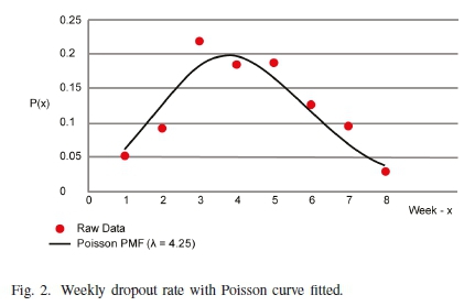
The initial study started with an investigation of past student failure in the advanced course on software design. The course was presented over one semester of 16 weeks. Historical data was collected for the 4 year period prior to the study described in the following sections, thus covering 8 semesters or 8 groups - Dataset 1. From the data collection process three distinct periods of failure were observed. The first was the dropout rate and covers a 8 week period at the start of the semester. During this time students are allowed to either register or deregister subjects. This period contributed 30%, on average, of the total student failure and the raw data in Fig. 2 is shown as a percentage of the average number of students that deregistered during this period. A Poisson distribution function was fitted with a mean λ= 4.25.

 

 

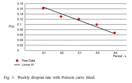
The second period spanned 10-14 weeks that overlapped with the first period. During this time students were required to submit assignments as part of the formative and continuous assessments, A1-A4 and E1, for this course. It was observed that this period contributed 35%, on average, of the total failure rate for all the students that enrolled for the course on a per semester basis. In Fig. 3 the average number of student omitting to submit assignments, is expressed as a percentage of the average number of students that failed during this period, is shown. A1-A4 are homework assignments and E1 a formal assessment done at approximately two week intervals.

 

 

The final period contributed another 9% to the total failure rate. This is due to student failing the end-of-term project and final evaluations. Thus the total pass rate for the subject only averaged 27%. This was alarming as this course followed on a prerequisite introductory course on software design. Although one could argue that the students lacked the required fundamental skills, the objective of the study was to expose the underlying factors that contribute to the processes that support student understanding and learning. The three periods of failure were combined into one graph showing the failure process as it occurred over the span of a semester, Fig. 4.

 

 

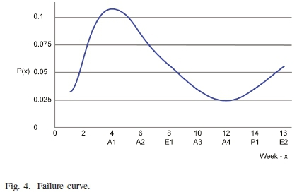
Deriving the failure curve concluded the preliminary research. The second period in failure curve, the attrition rate during weeks 4-14, was used as the central theme for the main study.

Measuring instruments and measures needed to be found to measure the underlying factors that contribute to the attrition rate, the second period of failure. These measures needed to contribute to the understanding of how the brain responds and assimilate new knowledge and skills. The development of these tools and measures are the topic of the next section.

 

III. Theoretical background - research design

The main research design was built in phases on the theories of analytic hierarchy networks and processes (AHN/P), the Guttman scale (GS), the just noticeable difference (JND) and various teaching and learning theories (TLT). The different phases are covered in the sub-sections below. The mathematical background was kept to a minimum in the main text and is presented in detail in Appendix A. The process here is a multi-stage instructional model [14] where:

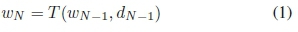
with the student being in State w_Nbased on the student's previous state w_N-1and the decision d_N-1. The new state is a function of both d and w denoted by T(w, d). The decision d_Nis calculated for each time interval and is dependent on the informal class assignments, A1-A4, and the formal assessment E1 as shown in Fig. 4.

A. The reference base measure

During the first class, the participants were required to complete a self-evaluation on how they perceived their own skill level of course material as mastered during the introductory course on software design. The objective of the self-evaluation was to establish a reference based on their performance during their participation in the prerequisite subject and was taken after successfully completing the prerequisite introductory course. The individuals' selections were totalled and averaged for the group. The individuals' selections were also cross-referenced with their actual performance for the course already passed.

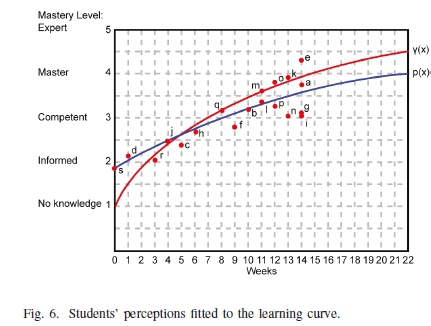
The process above resulted statistics being obtained for the perceived areas of good and bad performance. However, these statistics were skewed due to the primary fact that the students' level of mastery was in question. It was observed that students performed poorly during the first quarter of the advanced course on software design as students struggled with basic programming skills. Fig. 5 shows the sample data taken over a two year period of students' perceptions of their own abilities - Dataset 2. The Likert scales 3-5 (Know) is based on three knowledge levels: W - working knowledge, C - competent and E - expert. This was used to establish a reference base line and was used for the setup of the initial values of the study experiment variables, w₀in (1). The green blocks highlight the maximum selected perceived level. The orange blocks identify some ambiguous choices. The rank of the items is based on the maximum numbers as selected. The order is the sequence in which the items were presented. The statistics obtained gave the researcher some insight as to those areas which participants perceived that they had a lack in ability. The students' perception scores varied marginally from one year to the next.

Although the students' perceptions matched with their performance during the introductory course it did not reflect in their performance during the advanced course of software design. The works of Kruger and Dunning [20] shed some light in this regard. In their paper, they show how a person without true or valid knowledge is not able to recognise that their thought process and methods are in error. The statistics from this study affirmed the results as presented in [20] as students rated themselves higher than their actual skill level. The fields of study of software development and digital design require practitioners to make educated guesses and judgments of applying the appropriate algorithms to solve problems as well as the correctness of the code or a design as entered. This is a double blind dilemma situation as one needs to be an expert to make judgments, since as a novice you do not recognise your own lack of understanding and thus can only make limited judgments.

The previous performances of participants together with their perceived abilities were used as a reference measure w₀ on the one side and a guide to focus the tuitions to address possible problem areas on the other side. The perceived problem areas were redressed during the current course at the stages where the particular knowledge or skills were required based on d_Nfrom (1).

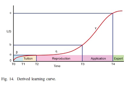
Fig. 6 shows the initial levels of the group at the start of the course fitted to the learning curve. γ(x) is the expected learning curve. p(x) is the fitted curve to the group average data. In the graph the use of the terms mastered and expert levels, as proposed by Dreyfus and Dreyfus [10], were swapped. The level of mastery here indicates that all aspects of the knowledge or skill is fully understood and the top level competency reached. Expert level here has the meaning of absolute mastery to the point where old rules and maxims can be re-evaluated and new rules and maxims be developed. This graph sets the base measure w0 from which any further development in knowledge and skill were measured.

 

 

B. The analytic hierarchy network

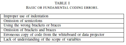
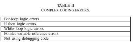
Next, data were collected of the typical errors made by students during the course. These programming errors consisted of both logical and syntax errors. In order to analyse the observations a measure needed to be constructed as the raw data were qualitative in nature. The transformation algorithm was based on the analytic hierarchy networks and processes (AHN/P) as developed by Saaty and Vargas [24]. Analytic hierarchy networks and processes are widely used in multicriteria decision-making techniques [21] and an example implementation can be found in [19]. Emrouznejad and Marra [11] provide a summary of the developments in AHP since 1979.

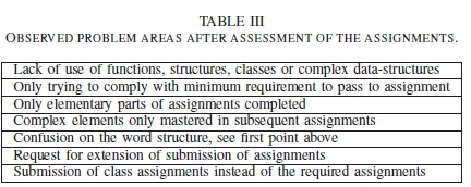
The main observations, Dataset 3, were grouped into formal sets. The sets are shown in Table I, Table II and Table III and were used to construct the analytic hierarchy network as proposed in [24], which is shown in Fig. 7. See Appendix A for a detailed mathematical perspective.

 

 

 

 

 

 

 

 

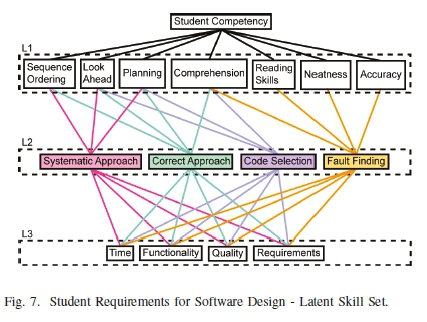
Level one, L1, is the first criterion level named the Fundamental Skills level for the purpose of this discussion based on the observations as discussed above. Level two, L2, is a tier higher in complexity, abstraction and mastery of the integration of the skill set listed on level L1, and based on the expected level of skill required to successfully complete tasks in the current course. The final tier, Level 3 (L3), is the highest level of abstraction and once more integrates all the levels below and is based on the requirements of a successful product. The purpose of this level is to describe the required product specification. Unlike the normal AHN, where the objective is of achieving most good or avoiding bad, in this study the goal was to understand the relationship between the different implementation activities of the processes of software design. The L1 criteria set was the first to be selected.

These criteria are different from the direct measure originating through the process of formal assessments e.g. the proper use and implementation of a for-loop. The criteria relate to the skills necessary to successfully complete the assignments and are thus latent, or secondary in nature, to the direct measure of expected outcomes. The C_L1set is listed below:

Reading skills (R) are the person's ability to fluently read through both the information communicated and the code produced. In coding this relates more to structure than the actual meaning i.e. syntax or structure and punctuation rather than semantics.

Comprehension (C) is the term used to describe a person's ability to understand what is communicated and respond in an appropriate manner, including appropriate comments.

Accuracy (A) is the inverse measure of how many mistakes are made by reading and retyping programming code or general generation of programming code.

Neatness (N) is the general layout and readability of the code, including appropriate comments.

Planning (P) is the overall design and design principles for the proposed solution.

Look ahead (L) is the ability to see possible restrictions or problem areas before they arise as well as issues such as data availability in time for processing.

Sequence ordering (S) is the appropriate ordering of program events so as to ensure proper performance measured to set expectations.

The L1 level criteria set was constructed from observations made during formal theory, tutorials, practical programming sessions and assessment of assignments. Formal observations were made and recorded on typical errors experienced by the participants. Most of the difficulties experienced by participants actually perpetuate from the prerequisite subject that precedes the one under investigation. The L1 criteria thus reflect the expected level of proficiency needed to be appropriately equipped to address problems and design software of the nature of the current subject under investigation. The next level, L2, is the Integrated Skill set C_L2:

To operate effectively on this level, L2, a software designer should ideally have mastered all the skills of L1. As these too are latent skills they are not directly measured but rather manifest as the cause of failure experienced when developing software. The C_L2skill set or criteria is listed below:

A Systematic Approach (SA) is a stepwise development procedure whereby each step has a specific role in the overall design procedure. Each step, though it precedes or follows other steps, is an independent abstraction of the total process. The rationale behind this methodology is that once a particular step concludes the steps following it have clearly defined input parameters.

The Correct Approach (CA) is the procedure that results in a final product that meets the expectation, following a near optimal route. With the term near optimal several other measures come into play such as: cost, time to develop, team size and minimal rework or redevelopment, as examples. This also relies on an excellent understanding of the project or product requirements.

The Code Selection (CS) refers to the appropriate selection of code to use in the implementation addressing the problem. Here one also refers to the functions, functionality and algorithms developed in the design process. There are many ways to implement possible solutions that may all work but some will be impractical and slow while others render neat and fast running code.

Fault Finding (FF) is the process of not only correcting compiler errors but also to identify and correct errors in the code or algorithms that was developed i.e. both syntax and logic errors.

The L2 level criteria were constructed from the level L1 criteria. The L1 level criteria were grouped to form an integration of fundamental skills into the next higher level skill. The L2 level criteria thus reflect both the higher cognitive level as well mastery and integration of the L1 level skills.

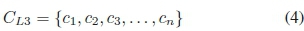
The final level is L3. This is the defined expected outcomes level. The measure of the final product is evaluated in terms of time efficiency, functionality, quality and the requirements set. The outcome criteria C_L3is given as:

Time Efficiency (T) is the total development time. This could also include factors such as team size in real-life development. Compliance with development schedules are the main measures though.

Functionality (F) is the overall features of the developed product. It also includes issues such as reliability, fully operational features, etc.

Quality (Q) is the subjective measure of the product in terms of the look-and-feel of the product. This includes ease-of-use and ease-of-learning of the product.

The Requirements (R) measure is a measure of how close the product adheres to the original set of requirements.

The next phase involved the matrix layout and capturing of the data - Dataset 4, the actual pair-wise comparison, expanding the AHN developed. An example implementation of pair-wise comparison can be found in [35]. The development here was based on the theory of comparative judgment introduced by Weber [34] in 1834, as presented in the paper by van der Helm [31], and further explored and expanded by Fechner [12] in 1860 and Thrustone [28] [29] in 1927. Stevens [26] [27] further explored their work in 1957. See Appendix A for a detailed discussion of the theories and mathematics involved.

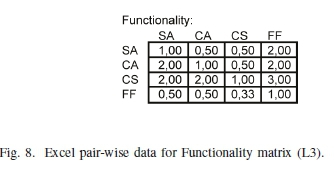
As an example of an AHN priority vector calculation we start with the pair-wise comparison matrix:

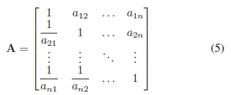
The example here shows a matrix that is populated with the pair-wise comparison data for the L3 tier - Functionality, as seen in Fig. 7. Fig. 8 shows one example matrix from Dataset 4 as captured in an Excel spread sheet. In the table the data is read as follows. For the row SA: the systematic approach (SA) is regarded as half as important when compared to the correct approach (CA) or code selection (CS). It is regarded as double as important as fault finding (FF).

 

 

This is followed by the calculation of the priority vector:

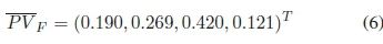
From the priority vector in can be concluded that the Code Selection (CS) takes on the highest priority with 0.420 out of the total scale of (0-1). Ranked second, the Correct Approach (CA) has a value of 0.269 followed by the Systematic Approach (SA) with a value of 0.190. Finally follows the Fault Finding (FF) and with a value of 0.107. The eigen value λ-max using the geometric mean method was calculated as λ-max = 4.070 and λ_max= 4.071 using Perron-Frobenius method.λ_maxis the greatest eigenvalue and for this type of matrix the other eigen values are all zero.

A third method is also proposed by the authors. Due to the fact that the values used in the comparative matrices are of the same range (1-9), a normal-average taken over the rows of the normal-matrices resulted in a priority vector with similar values to the geometric mean method. Using this method λ_max= 4.078 and a priority vector:

This new vector also adds to 1 when all its components are summed in accordance with the geometric mean method. For:

This procedure above was followed for level L2 and L3 as shown in Fig. 9, a total of 16 matrices and their related priority vectors. These were collated in a spread sheet table shown in Fig. 9 relating tier L1 with tier L3 from Fig. 7.

 

 

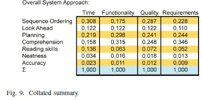
The collated data is a summary of all the priority vectors that are used in the decision making processes. From the collated data and resulting calculations the following observations can be made.

For the effective management of time or timeous delivery of a solution or product, Sequence ordering plays the most important role followed by Planning;

To produce a solution that is Functional, i.e. contains operational or working modules, Comprehension or understanding of both the problem and possible solutions plays the most important role followed by Planning;

Where the solution or product Quality is concerned, Sequence Ordering is just ahead in importance followed closely by Planning and Comprehension;

As far as the project Requirements are concerned Comprehension is again the determining factor followed with a tight second place by Planning and Sequence Ordering; and

The roles of Reading Skills, Neatness and Accuracy play their most important role in the Time domain i.e. a direct influence in the development time of application code.

The collated data as given in Fig. 9 now became the input for the tuition management phase. The objective was to forward a model that will highlight the underlying factors that contribute to learning. The learning model derived in this paper consists of the Time component as the diminishing resource split between the Systematic Approach, Correct Approach, Code Selection and Fault Finding using the L2-L3 priority vector as a weight vector. The time resource is thus divided into the four parts, as a time budget for each component, using the weight vector as guide:

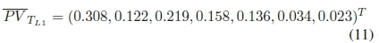
On the L1 tier the Time priorities are divided between Sequence Ordering, Look Ahead, Planning, Comprehension, Reading Skill, Neatness and Accuracy using:

This priority vector was used to manage the time spent on writing code for assignments. Students were encouraged to follow the suggested time schedule as a more effective means of utilising the diminishing time resource. For an assignment 12 hours are budgeted and is divided amongst the activities of L1 using the priority vector. Using planning as an example, 21.9% or 0.219 χ12 = 2.628 hours of the total 12 hours, as budgeted, is to be spent on this activity to ensure successful completion of the project. These are guidelines that need to be adjusted as the project progresses.

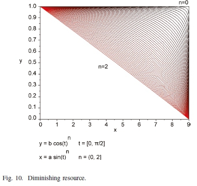
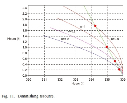
Using the schedule an early warning system is developed. The span of an assignment is 2 weeks or 336 hours. Leaving the project for the final 12 hours of the two week period usually results in failure to deliver the completed assignment. Equation (12) describes time as a diminishing resource. a is the period over which the resource is utilised. b is the initial value of the resource to be utilised.

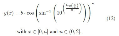
Different time utilisation paths were modelled using (12). In Fig. 10 we can see by varying n between 0 and 2 the time utilisation path can be linear (n = 2), exponential (n = 1.656) or a step function (n - 0), for one unit of the resource being utilised over a period of nine intervals. In Fig. 11 several example failure points are shown. Each of the intersections is a critical point of failure to be avoided to ensure success, i.e. left of the straight line is the 'safe' side.

 

 

 

 

The question now is how do we define adequate time as needed to successfully complete the assignment by the majority of the students?

C. Time-on-Task

In the endeavour to understand the time-on-task relations, between the presentation of study materials and the mastery thereof, two further measures were introduced to try and expose the main contributors of failure in the advanced course on software design. The first was a measure of the number of students that gained basic understanding of material over a period of time. The second was a measure of average time it took students to master a topic i.e. measure how long does it takes to attain different levels of mastery in a specified topic using assignments and formal assessments as measuring instruments.

There are 7 formal assessments throughout the semester and numerous in class assessments almost every contact period. Each class spans 3 hours and is divided amongst theory and practical demonstration presented by the lecturer, 1 hour, and in class assignments done by the students, 2 hours. These measures, Dataset 5, were used to construct the new learning curves that follows. The data involved is numerous and thus only summaries and examples sets are presented here.

The process of measurement involved the monitoring of students' progress when new topics were introduced as well as documenting the typical questions asked and mistakes made by students. The formal evaluation involved repeated measures of a specific topic until it is evident that students have mastered the specific topic.

The different topics of the course material are structured in a layered structure i.e. similar to the nested Russian folk dolls (Matryoshka dolls) where the inner layers are the fundamental knowledge and the outer layers more complex in nature. This method ensures that knowledge and skills introduced at an earlier stage are exercised over and over until mastery is achieved. This is in line with the concept measure scale developed by Guttman [15]. For the detailed mathematical development see Appendix A. The inner layers are included in the outer ones, i.e. a piece of knowledge or a skill mastered at an inner level is embedded into the one on the outer layer.

In Fig. 12, two examples of different topics, as they were covered in the course on advanced software design, are shown for the number of students mastering the basic skill level of Novice. The sample shown is for a sub-sample of 108 students collected over a two year period. The example topics shown here cover two different difficulty levels ranked according to the time period it took students to master the fundamental knowledge or skill, Example 1 an easy topic and Example 2 a more difficult topic. The graphs show the number of students per session that transcend from having no knowledge or skill to understand the fundamental concepts. A session being a class or other formal contact period between instructor and students. The two graphs for each of the examples consist of: a raw data graph i.e. the student count tabulated during a particular session and a cumulative graph over a period of time. As the topics grow more difficult the distribution graphs flatten out as the students take an increasingly longer time to master the fundamental work.

 

 

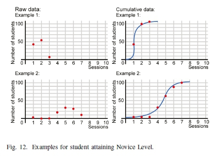
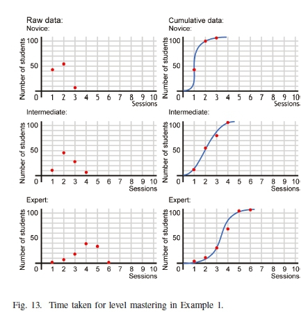
Fig. 13 shows the progression of the students over time for the Example 1 topic i.e. how well have they mastered the topic at hand. The time interval covers the three periods Novice, Intermediate and Expert level of mastery. For each level two graphs are shown: the raw student count tabulated per session and the cumulative graph over a period of time. The periods of transcending each of the levels vary widely between topics and are dependent on the difficulty of the topic. There is a general spread of the time required to master each of the mastery levels. This is an indication of how long it will take the average student to transcend to the next level. The average student value is obtained by calculating the mean of the tabulated sum of the number of students for the indicated time periods. A different measure could be to use 80% of the students as a reference to include as many candidates as possible or for specialised courses only 10% of the students as a means of selection.

 

 

A summary of the data obtained for four different topics are given in Table IV. The first two topics are equivalent in nature and difficulty and may be presented in any order. The second topic is always mastered in a shorter period than the first one as students have already mastered the related first topic. The third and fourth topics are always presented in the same order as the third topic is the precursor to the fourth topic. The different time intervals are shown as indicated in Fig. 14. The first period T₀ - T₂is the instruction time for the topic. This includes theory and examples done by the lecturer. The second period T₂- T₃is the average time needed by 80% of the students to demonstrate their mastery of the fundamental skills. The final period T₂ - T₃is the average time needed by 80% of the students to demonstrate their mastery of the advanced skills for a specific topic.

 

 

 

 

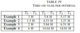
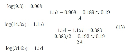
Furthermore, it was observed that when comparing the logarithm (13) of the time-on-task measurements in Table IV, an interval difficulty scale is derived on which the topics can be placed and compared with each other. using this scale as statement like "Example 4 is twice as difficult as Example 3 or three times as difficult as Example 2." has a sound mathematical construct. This is in accordance to the scale developed by Stevens as discussed in Appendix A.

In related studies on crows, Ditz and Nieder [9] found that birds' ability to distinguish between different number of food objects varied on a logarithmic scale as suggested by the Weber-Fechner Law. This would suggest that the way in which the animal brain perceives and reacts to stimuli are hardwired accross species[A].

These results were used in the time-on-task restructuring processes for the re-curriculation of the material in the advanced course on software design.

D. The learning curve

From Table IV two new generalized equations describing the learning curve were derived:

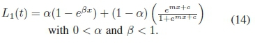
or

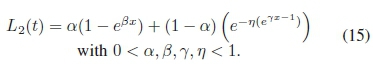
Where αis the height of the first plateau, βis the learning rate during the first period, γ is the slope for the second period and ηis a time position related variable of where the final learning plateau starts. These equations were used to plot the learning curve in Fig. 14. combining the failure distribution Fig. 4 with the learning curves for E₁ - E₄we have Fig. 15

 

 

From Fig. 15 it can be seen that the first evaluation A₁ only takes places once the students have mastered topic 1 (Ei) and topic 2 (E₂). The high rate of failure was mainly due to students either cancelling the course or adjusting to the expectations of the advanced course. From evaluation A₃onwards students were confronted with having to do the assignment although they have only acquired the competent level on the learning curve for the required skill level as described by the curve E₃. The relative low failure rate at this point can be contributed to two main factors. The first is that most of the struggling students have been 'weeded' out. The second factor can be contributed to the fact that the fundamental knowledge is well mastered at this point and students are able to bridge the education gap by themselves.

 

IV. IMPLEMENTATION

During the implementation phase two concepts are introduced. The model presented in this paper also includes the electrical engineering core structure as a whole. Therefore, we introduce the time-on-task inter-subject relations as pertaining to the prediction of impending failure. In order to give appropriate guidance to students a study was needed to understand the influence between subjects with regard to the probability of failure of subjects in relation to the average mark for the subjects involved. Finally the Rope-Weaver's Principles are derived.

A. Decision boundaries

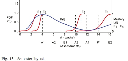
The data used to develop the failure risk model was obtained from historical student results using the methods described above - Dataset 6. Students were enrolled for the first semester of their first year in engineering studies, with field of specialization Electrical Engineering, for a specific year. Only those students that took the full complement of subjects, six subjects, where considered, a total of 186 students. The results were tabulated per student per subject. Intermediate results were averaged to use as indicator variables. Table V contains the average mark after the first assessment. The first group consisted of all the students that failed one subject at the end of the semester. A total of 26 students failed one subject during the semester, or « 14% of the total number of students. The second group passed all six the subjects at the end of the semester but had one or more subjects with a final mark of 50-53%. A total of 19 students almost failed one subject, or » 10% of the total number of students. Thus these two groups together constitute « 25% of the population. This is the total number of students that are in the threshold or danger area, i.e. 45 students out of the total number of 186 students.

 

 

The left side of the table is the average mark for those students taking the full complement of six subjects but failed one of them. The right side of the table is the average mark per student taking the full complement of six subjects but having one or more subjects with a mark of between 50-53% i.e. were in danger of failing a subject.

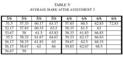
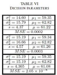
From data in Table V a scatter plot was constructed which is shown in Fig. 16. The scatter plot contains the data for the students that failed one subject at the bottom of the figure and the data for the students that almost failed a subject at the top of the figure. Assuming normal distributions for both, the parameters for the probability density functions (PDFs) are calculated using standard procedures and the results are summarized in Table VI where and μ_ιare the parameters for the probability density function (PDF-\) of passing 5/6 subjects. σ| and μ₂are the parameters for the probability density function (PDF₂) of passing 6/6 subjects. The cumulative distribution function (CDF) is calculated as:

 

 

 

 

 

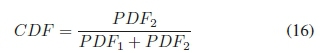
The CDF can be modeled assuming a logistic distribution:

 

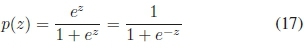
with:

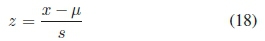
x represents the independent variable of the average marks obtained. μis the mean value for the CDF. s is a parameter related to a²for the normal distribution.

The top entry in Table VI assumes a²and μto be calculated from the population mean. The middle entry assumes and μto be calculated from a sample mean. The bottom entry assumes and μto be calculated from a sample mean with al and , equal. In each of the three examples in Table VI, μand s for the CDF were calculated using linear regression techniques. The mean-square-error (MSE) for each example is also shown. MSE in the top two examples are much higher as the two PDF distributions are not equal in nature as is the case with third example.

The failure risk threshold was thus calculated as 61.08%. Having an average mark of 61.08% over all six subjects, gives a student a 50% chance of failing one subject. This threshold value is then monitored as part of the time scheduling subsystem that is implemented as an analytic hierarchy network (AHN) or process (AHP). The threshold now becomes our basis for the decision d_Nfrom (1) to establish the next state w_nfor each of the students.

B. Decision example

At the start of a semester students need to assess the amount of time to spend outside of class on each subject. It is a formal requirement that classes, tutorials, practical classes and formal assessment consume 100 hours per subject each semester. These include all lectures, tests and practical evaluations, but excludes formal exams at the end of the semester, over a 16 week period. Two of these weeks are used for formal tests and other evaluations leaving 14 weeks of class. On average formal assessments and feedback consume 30 hours, leaving 70 instructional hours. Thus, a student taking 6 subjects, spends 5 hours in formal instruction per week per subject for a total of 30 hours per week. It is universally accepted that a student should spend on average 1 hour studying outside of class for each hour spent in class. As a base line, a student needs to spend an additional 5 hours a week per subject on their studies.

Not all subjects are equal in nature, as some require more attention than others. So too are the skills and knowledge of students not equal in all fields of study or amongst each other. Subjects do not necessarily have other subjects that follow after them or follow on from a previous subject. One can thus not apply a fixed rule to all students and all subjects alike. Students will use their belief system based on past experience, sometimes also on the experience of past students, to make an 'informed' judgment on the perceived difficulty of subjects, L1.

From the discussions above the developed advisory system requires two inputs. The first is the informed judgments as to the perceived difficulty of the six subjects taken in the first semester. This will be different for each of the candidates. The comparative judgments are done in accordance to the process as suggested by Guttman. The second input is the threshold limit as obtained from the historical data of the students as discussed above. The subjective ordinal scale comparative judgments are then transformed into the first iteration interval scale priority vectors using the AHN approach as suggested by Saaty [24]. The perceived difficulty judgments for the vector L1 is calculated next.

The following is an example of one of the students perceived difficulty levels. Fig. 17 shows the data as captured in a spread sheet. This is initial data for our matrix used to calculate the priority vector using the methods discussed above.

 

 

 

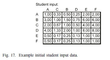
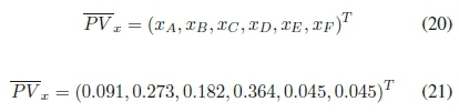
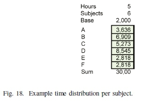
From the priority vector it can be seen that subject D has the highest priority and subjects E and F the lowest priorities. The priority vector is now employed to calculate the appropriate time to be spent on each of the subjects during home study. The prescribed 5 hours, h, per subject during home study is now divided into two parts, the base time plus the priority time. The base time is selected as the absolute minimum time for each of the subjects, m in total. The base time, b, for the purpose of this example is set at 2 hours per week. The other 3 hours are assigned based on the priority vector. The time allocation formula is then:

From Fig. 18, it can be seen that the subject 'regarded' as most difficult is now charged with 8.5 hours for study, outside of the formal programme, while the easiest subject with 2.8 hours weekly. Now the student has a guideline as to a possible schedule, hours to be spent, for each of the subjects.

 

 

After a period of time the first assessment is done to assess the progress of a student for each of the subjects. The process of assessment here could be in the form of class tests or assignments. The results obtained from the assessments, Dataset 7, are fed back into the advisory system and the priorities reassessed and appropriately adjusted for the next time period.

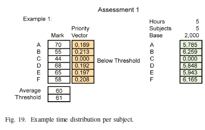
To demonstrate the process two examples are given covering two different scenarios for the threshold function. The results obtained from the review process were tabled and ranked. The priorities were then focused on the 'problem' areas as can be seen from the priority vectors in Fig. 19 and Fig. 20. The Guttman scale, however, does not directly translate into the adjusted priorities and therefore a transformation function was needed. The new priorities are now calculated using the mean value to first obtain a normalised displacement:

 

 

 

 

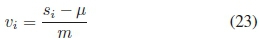
Where s_iis the assessment value for subject i and m the number of subjects under review. The priority vector is now calculated:

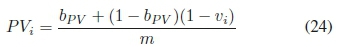
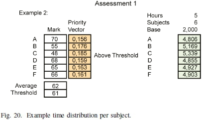
With b_PV= [0,1], the baseline, for the priority vector. Two examples are shown in Fig. 19 and Fig. 20 respectively. The baseline b_PVwas set at 0.5 for these examples.

Fig. 19 shows subject C with a zero priority. This is due to the threshold elimination that was implemented as the average mark for the six subjects was below the threshold of 61%. The function of the threshold in this case is to suggest a decision to eliminate, or deregister, subjects in which there is only a slim possibility of success. A similar process will be followed in other implementations where a service or product will be eliminated, culled, from further calculations to avoid cascading failure. The threshold is based on the average probability as measure, the raw test scores, and calculated, transformed into priority vectors, as discussed above. Subjects below the threshold are eliminated from any further calculations i.e. the subject is deregistered. From the subject priority sequence we now have:

There are several ways to deal with the 'additional' 5 hours per week that become available after the elimination of subject C. Normally it just gets absorbed by other activities and not necessarily by academic activities. Another option is to keep the time in reserve to compensate for other disruptions and interruptions. A third option is to utilise the 'spare' time by distributing it amongst the five remaining subjects. The time distribution in Fig 19 illustrates the latter using (21) as reference.

Fig. 20 illustrates the case should average mark fall above the threshold and no subjects are deregistered. The focus now shifts to subject C followed by subject B and so on. It is interesting to note that much time has been spent on subject D that was considered as most difficult or vulnerable and has been mastered and thus is now almost considered an easy subject. The process above is repeated for each review until the end of the term is reached guiding the student with suggestions on how to manage their studies. Review here refers to any form of assessment, formative or summative, after which the students ought to receive feedback in a timely manner.

As can be seen from this study a large portion of students, 24%, fall into the 'danger area' of which 14% actually failed one subject out of the full complement of six subjects. With support and guidance the 14% students that failed one subject could potentially be rescued. Only 39% of students taking the full complement of subjects, six first year subjects, passed all six. If the 14% can successfully be helped the success rate could be improved to more than 50%, an improvement of almost 36%. This will lead to improved throughput throughout the programme as the techniques discussed here are implemented on all levels of study.

C. The Rope-Weaver's Principles

The Rope-Weaver's Principles were formulated based on the observations discussed above as an abstraction of the underlying mathematical principles and measures, also in [4]. The Rope-Weaver's Principles thus become a set of rules or guides for enhancing learning. The title "The Rope-Weaver's Principles" is being used as a metaphor for the processes of teaching and learning. In the Rope-Weaver metaphor the different strands or fibers are spun together into threads. The strands and fibers are the basic building blocks that constitute a topic. Some are dependent and others are independent. They are all just loose ideas until spun together into a thread or topic. Different threads are woven into yarns. Yarns constitute the broader study themes. The yarns are finally woven into the final rope structure. The rope structure is akin to subjects or fields of study, Fig. 21.

 

 

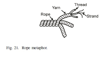
The first principle assumes that each new level of mastery, new knowledge or skills encompasses all the ones that it relies on e.g. one need to first learn how to add single digit numbers before one can add two digit numbers and so on. This is in line with the Guttman scale. This is the layered structure as discussed in the research overview above. In this model, the simple rule-based or novice levels lie in the centre and the more advanced, maxim or expert levels, on the outer levels. This is also equivalent to the different layers found in a rope. Each new layer builds on the layers below to determine the strength of the overall rope.

The second principle is to postpone the introduction of a new topic until most students have entered into the Intermediate level of mastery in the previous topic. The rationale behind this is born from the work of Johnson-Laird et al [18]. If the step between the new topic and the mastered topics is too great, the challenge to recognise, understand or master the fundamental knowledge or skills is masked by the impulse generated by the introduction of the material itself i.e. you simply cannot discern a 100 g weight form a 101 g weight as was found by Weber [34]. This principle is known as the just noticeable difference. It deals with the brain's inability to sense small differences in stimuli. An example implementation of the just noticeable difference can be found in [33].

It is expanded on here to include the brain's inability to rely on or recall known information when confronted with new knowledge far removed from the current experience. This relates to the example that students refer to as 'striking a blank'. This so-called blank is the result of not being adequately prepared and then being confronted with some questions far removed from their field of experience. The resulting overload by the stimulus now even masks all the 'easy' material that is mastered.

This is also the main driving force behind the third principle, breaking the work that must be mastered during a course into small enough steps. The rationale is, as explained above but additionally, to support shorter intervals between the introduction of new materials or skills. Some of these sub-topics are not interdependent and may be reordered as proposed in the Fourth principle.

The fourth principle is the 'parallel' or staggered introduction of non-dependent materials or skills. The rationale here is, as a prior topic's mastery matures, a new unrelated topic may be introduced. It was found during the study that unrelated topics may be introduced in parallel without any negative effects on the other topics in the process of being mastered. The mastery of these unrelated topics can now mature at the same time. Furthermore, closely related topics are presented in short succession so as to keep the apparent gap between topics introduced as small as possible. This is similar to the construction of a rope as new strands and fibers are introduced, and spun into the same thread, as the rope is woven.

The fifth and final principle is the process of facilitating the transcendence from ignorance to intermediate level. During the initial phase the novice needs to be coached as the novice operates optimally using a set of rules, rule-based learning -Behaviourism. This means that the rules need to be drilled until they become mastered to the point of second nature. The second phase, transcending from novice to intermediate level, is concerned with the introduction of maxims - Constructivism and the principles of scaffolding knowledge and skills. The boundaries of the rules need to be enlightened or exposed. As the students progress in this phase they will enter into the state of self-motivation. They will start to explore on their own. This is the transcendence into the expert level. This is our goal.

 

V. Conclusion

The main results observed are summarised in Fig. 22. The failure curve P(t) is shown at the furthest point and was constructed from the student behaviour data. The graph L(t) is the progression graph of moving from a rule-based cognitive level to a maxim-metacognitive level. The measured learning curves for several example topics, E\ - E₂are plotted in relation to these two graphs at their respective points of origin as presented within the course.

It was further observed that it takes exponentially longer to master the more advanced topics that require one to operate at the metacognitive level. From the discussions above and the results from this study, these suggest that the process of acquiring new knowledge or skills is hard-wired in the brain [2] and conforms to the Weber-Fechner Law. When students are confronted with tasks that they are familiar with, they experience no problem solving and completing the tasks. As these tasks are further removed from their experience, they exponentially experience more difficulty in completing the tasks. It can thus be concluded that with more directed effort during the plateau phase the time period for this phase can be reduced leading to accelerated or more effective learning.

The measurement of the threshold region for potential student failure forms a critical component in the data transformation process of the subjective student comparative judgements, ordinal scale data, into objective priority vectors, interval scale data. The advisory system data collection and transformation was done using the methods suggested by Guttman and Saaty. The interval scale priority vectors were successfully used by the advisory system to calculate the time distribution values.

The main benefit of this study lies in the objective support and guidance that this system provides when students are given feedback in a timely manner. The transformation of raw subject scores into objective decision vectors remove students from ambiguous perspectives and making wrong decisions. This is implemented using the Rope-Weaver's Principles to address the problem areas through a process of developing new curriculums and are based on the theories of analytic hierarchy networks and processes (AHN/P), the Guttman scale (GS), the just noticeable difference (JND) and various teaching and learning theories (TLT).

This study is also applicable to other projects or processes where there are a mixture of shared non-renewable resources and renewable resources. Examples include products or services that may be discontinued due to profitability or some other measure. The criteria for the decision to cull parts of the project will differ but the main decision process remains common to all applications.

 

Acknowledgement

The authors convey their gratitude to Tshwane University of Technology for their financial and resource support.

 

References

[I] K. Anicic, B. Divjak, K. Arbanas, " Preparing ICT Graduates for Real-World Challenges: Results of a Meta-Analysis," IEEE Transactions on Education, vol. 60 , no 3 , pp.191-197, Aug. 2017 . DOI: 10.1109/TE.2016.2633959        [ Links ]

[2] R. C. Aylward, "Engaging the student: Programming solving real-life problems," in IEEE AFRICON 2013, Mauritius. 9-12 Sep. 2013, pp. 85585. DOI: 10.1109/AFRCON.2013.6757779

[3] R. C. Aylward, "Hardwired: Facilitating engineering studies," in South African Society for Engineering Education (SASEE) 2017. Engineering education in transition: Responding to a changing higher education landscape, Cape Town, South Africa, Jun. 2017. [Online]. Available: https://www.sasee.org.za/wp-content/uploads/Proceedings-of-the-4th-Biennial-SASEE-Conference-2017.pdf

[4] R. C. Aylward, "Learning Curves: Insights and conflicts towards more effective learning," in IATED 11th International Conference ofEducation, Research and Inovation, Seville, Spain, 12-14 November, 2018. DOI: 10.21125/iceri.2018.1423

[5] N. Burch, "Four stages of competency," Gordon Training International, 1970's. [Online]. Available: http://www.gordontraining.com/free-workplace-articles/learning-a-new-skill-is-easier-said-than-done/

[6] Centre for Development and Enterprise (CDE). "The maths and science performance of South Africas public schools: Some lessons from the past decade," Johannesburg: Centre for Development and Enterprise, 2010. [Online]. Available: https://www.africaportal.org/documents/2596/Maths_and_Sci-ence_Performance_Some_lessons_from_the_last_decade.pdf

[7] Council on Higher Education (CHE). "Higher Education Monitor 9: Access and Throughput in South African Higher Education - Three Case Studies," Council on Higher Education, Pretoria: Council on Higher Education, 2010. [Online]. Available: https://www.che.ac.za/media_and_publications/higher-education-monitor/higher-education-monitor-9-access-and-throughput

[8] Department of Education (DoE). "Curriculum 2005: Lifelong Learning for the 21st Century," National Department of Education, Pretoria: Government Printers, 1997. [Online]. Available: http://hdl.voced.edu.au/10707/107848

[9] H. M. Ditz and A. Nieder, "Numerosity representations in crows obey the Weber-Fechner law," Proc. R. Soc. B, 283, 2016, DOI: 10.1098/rspb.2016.0083        [ Links ]

[10] S. Dreyfus and H. Dreyfus, "A five-stage model of the mental activities involved in direct skill acquisition," Operations research center, Univ. of California. Berkeley, 1980. [Online]. Available: http://www.dtic.mil/dtic/tr/fulltext/u2/a084551.pdf

[11] A Emrouznejad and M Marra, "The state of the art development of AHP (1979-2017): a literature review with a social network analysis," International Journal ofProduction Research, vol. 55, no. 22, pp. 66536675, 2017. DOI: 10.1080/00207543.2017.1334976        [ Links ]

[12] G. Fechner, "Elemente der Psychophysik," Breitkopf und Hartel, ETH- Bibliothek, Zurich, Rar 5285, 1860. DOI: 10.3931/e-rara-10879 [13] G Fisher, "Improving Throughput in the Engineering Bachelors Degree. Report to the Engineering Council of South Africa." October 2011. [Online] Available https://www.ecsa.co.za/about/pdfs/091211_ECSA_Throughput_Report.pdf

[14] G.J. Groen and R.C. Atikinson, "Models for Optimizing the Learning Process," Psychological Bulletin, vol. 66, no. 4, pp. 309-320, 1966. [Oniline]. Available: http://rca.ucsd.edu/selected_papers/ModelsforOptimizing the Learning Process_Psychological Bulletin_October 1966.pdf        [ Links ]

[15] L. Guttman, "A basis for scaling qualitative data," American Sociological Review, vol. 9, no. 2, pp. 139-150, 1946. DOI: 10.2307/2086306.         [ Links ]

[16] L. Guttman, "An approach for quantifying paired comparisons and rank order," The Annals ofMathematical Statistics, vol. 17, no. 2, pp. 144-163, 1946. DOI: 10.1214/aoms/1177730977.         [ Links ]

[17] S. Hanna, H. Jaber, A. Almasalmeh and F. Jaber, "Reducing the Gap between Software Engineering Curricula and Software Industry in Jordan," Journal ofSoftware Engineering and Applications, no. 7, pp. 602-616, 2014. DOI: 10.4236/jsea.2014.77056        [ Links ]

[18] P. Johnson-Laird, P.N. Legrenzi and M. Legrenzi, "Reasoning and a sense of reality," British Journal ofPsychology, vol. 63, pp. 395-400, Aug. 1980. DOI: 10.1111/j.2044-8295.1972.tb01287.x.         [ Links ]

[19] J. Krejcí, D. Petri and Michele Fedrizzi,"From Measurement to Decision with the Analytic Hierarchy Process: Propagation of Uncertainty to Decision Outcome," IEEE Transactions on Instrumentation and Measurement, vol. 66, no. 12, pp. 3228-3236, 2017. DOI: 10.1109/TIM.2017.2749798        [ Links ]

[20] J. Kruger and D. Dunning, "Unskilled and unaware of it: How difficulties in recognizing one's own incompetence lead to inflated self-assessments," Journal of personality and social psychology, vol. 77, no. 6, pp. 11211134, 1999. DOI: 10.1037//00223514.77.6.1121.         [ Links ]

[21] M. Martinez, D. de Andres, J.-C. Ruiz and J. Friginal, "From measures to conclusions using analytic hierarchy process in dependability benchmarking," IEEE Transactions on Instrumentation and Measurement, vol. 63, no. 11, pp. 2548-2556, Nov. 2014. DOI: 10.1109/TIM.2014.2348632        [ Links ]

[22] I.N.S Mullis, M.O Martin and T. Loveless, "20 Years of TIMSS International Trends in Mathematics and Science Achievement, Curriculum, and Instruction," International Association for the Evaluation of Educational Achievement (IEA), 2016. [Online]. Available: http://timss2015.org/timss2015/wp-content/uploads/2016/T15-20-years-of-TIMSS.pdf

[23] K. Pearson, "On the theory of contingency and its relation to association and normal correlation," Drapers' Co. Memoirs, Biometric Series London, vol. 1, 1904. [Online]. Available: https://archive.org/details/cu31924003064833

[24] T. L. Saaty and L. G. Vargas, "Decision-making with the Analytic Network Process: Economic, Political, Social and Technological Applications with Benefits, Opportunities, Costs and Risks," vol. 195 of International Series in Operations Research & Management Science, Springer, second ed., 2013. DOI: 10.1007/978-1-4614-7279-7

[25] N. Spaull, "South Africa's education crisis : The quality of ducation in South Africa 1994 - 2011," Johannesburg: Centre for Development and Enterprise, 2013. [Online]. Available: http://www.section27.org.za/wp-content/uploads/2013/10/Spaull-2013-CDE-report-South-Africas-Education-Crisis.pdf

[26] S. S. Stevens, "On the psychophysical law," Psychological Review, vol. 64, pp. 153-181, 1957. DOI: 10.1037/h0046162.         [ Links ]

[27] S. S. Stevens, "To honor fechner and repeal his law," Science, New Series, vol. 133, pp. 80-86, Jan 1961. DOI: 10.1126/science.133.3446.80.         [ Links ]

[28] L. Thurstone, "Psychophysical analysis," The America Journal ofPsy-chology, vol. 38, pp. 368-389, Jul 1927. DOI: 10.2307/1415006        [ Links ]

[29] L. Thurstone, "A law of comparative judgment," Psychological Review, vol.34, pp.273-286, Jul 1927. DOI: 10.1037/h0070288.         [ Links ]

[30] K. Tsukida and M. Gupta, "How to analyze paired comparison data," UWEE Technical Report Number UWEETR-2011-0004, May 2011. [Online]. Available: http://www.dtic.mil/dtic/tr/fulltext/u2/a543806.pdf

[31] P. A. van der Helm, "Weber-Fechner behavior in symmetry perception?," Attention, Perception, & Psychophysics, vol. 72, no. 7, pp. 1854-1864, 2010. DOI: 10.3758/APP.72.7.1854        [ Links ]

[32] C. van Wyk, "An overview of Education data in South Africa: an inventory approach," Stellenbosch Economic Working Papers: 19/15, Department of Economics, University of Stellenbosh, 2015. [Online]. Available: https://www.ekon.sun.ac.za/wpapers/2015/wp192015/wp-19-2015.pdf

[33] S. Wang, L. Ma, Y. Fang, W. Lin, S. Ma and W. Gao, "Just Noticeable Difference Estimation for Screen Content Images," IEEE Transactions on Image Processing, vol. 25, no. 8, pp. 3838-3850, 2016. DOI: 10.1109/TIP.2016.2573597        [ Links ]

[34] E. H. Weber, "De pulsu, resorptione, auditu et tactu [On stimulation, response, hearing and touch]," Annotationes, anatomicae et physiologicae, Leipzig, Austria: Koehler, 1834. [Online]. Available: https://hdl.handle.net/2027/njp.32101067214807

[35] H. Yin, X. R. Li and J. Lan, "Pairwise Comparison Based Ranking Vector Approach to Estimation Performance Ranking," Systems IEEE Transactions on Systems Man and Cybernetics, vol. 48, no. 6, pp. 942953, 2018. DOI: 10.1109/TSMC.2016.2633320        [ Links ]

 

 

R.C. Aylward is with the Department of Electrical Engineering, Tshwane University of Technology, Pretoria, South Africa (e-mail: ayl-wardrc@tut.ac.za).
B.J. van Wyk is the Executive Dean of the Faculty of Engineering and the Built Environment, Tshwane University of Technology, Pretoria, South Africa (e-mail: vanwykb@tut.ac.za)
Y. Hamam is a Professor with the Department of Electrical Engineering, Tshwane University of Technology, Pretoria, South Africa and Emeritus Professor at ESIEE-Paris, France (e-mail: hamama@tut.ac.za)

 

 

 

Ronald Charles Aylward (M'18) has been a lecturer at the School for Electrical Engineering, Tshwane University of Technology, Pretoria, South Africa, since May, 1993. He holds a MTech degree in Electrical Engineering, Digital Technology from the Tshwane University of Technology, South Africa, a B.Sc.Hons. in Computer Science and a B.Eng in Electronic Engineering from the University of Pretoria, South Africa. His fields of specialisation are: Advanced Processors, AI, Modelling and Engineering Education. He has authored and co-authored papers in several journals and conference proceedings. He has been an active reviewer for several Journals including IEEE Transactions on Education for many years.

 

 

Barend Jacobus van Wyk (M'03) has a passion for technology and the demystification and communication of complex technological, scientific, educational and management concepts in a novel and fun way. He is also a Research and Innovation Professor at the Tshwane University of Technology and the Executive Dean of the Faculty of Engineering and the Built Environment. He obtained his PhD from the University of the Witwatersrand, has more than 12 years of industrial experience in telecommunications and aerospace engineering, and is an NRF (RSA) C2 rated researcher who published more than 120 peer reviewed conference/journal papers since 1998. His research interests are telecommunication networks, signal processing, machine intelligence and control, image processing, pattern recognition, aerospace engineering and engineering education.

 

 

Yskandar Hamam (M) received the bachelor's degree from the American University of Beirut in 1966, the M.Sc. and Ph.D. degrees from the University of Manchester Institute of Science and Technology in 1970 and 1972, respectively, and the "Diplome d'Habilitation a Diriger des Recherches" degree from the Universite des Sciences et Technologies de Lille in 1998. He conducted research activities and lectured in England, Brazil, Lebanon, Belgium, and France. He was the Head of the Control Department and the Dean of the Faculty with ESIEE Paris, France. He was an Active Member in modeling and simulation societies. He was the President of EUROSIM. He was the Scientific Director of the French South African Institute of Technology, Tshwane University of Technology (TUT), South Africa, from 2007 to 2012. He is currently a Professor with the Department of Electrical Engineering, TUT and Emeritus Professor at ESIEE-Paris, France. He has co-authored three books. He has authored or co-authored over 300 papers in archival journals and conference proceedings and book contributions.

 

 

 

Appendix A Detailed theoretical background

The purpose of this discussion is three-fold. Firstly, these theories were used to develop the research goals. Secondly, the theories were used to develop the procedures to process the data to obtain measures. Lastly, the theories are provided as background for the discussion of the results.

A. Comparative Judgment

Weber [34] described experiments involving human sensory systems in his 1834 book. One of the experiments was aimed at determining the just noticeable difference (JND) perceived by an observer when evaluating the difference between two weights. He determined that a subject could distinguish between a 20 g weight and a 21 g weight but not a 20.5 g weight. Furthermore as the weights in the experiment grew in weight the noticeable difference grew in size i.e. a subject could only distinguish between 40 g and 42 g, a 2 g step. He defined the difference as a dependent of the weight by some constant factor K.

Building on the work of Weber, Fechner [12] actually laid down the mathematical foundations for (27). It is referred to as Weber's constant or Weber's Law. Fechner expanded Weber's work into a series of just noticeable stimuli:

Furthermore, Fechner found that Weber's Law holds for ranges of s where s is relatively small compared to s. Finally Fechner arrived at an equation for the perceived magnitude P and the stimulus I:

K being Weber's constant above. This means that the intensity of the stimulus needs to be tenfold to be perceived as double the original intensity, log(10) = 1, log(100) = 2. Stevens in his papers [26] [27] further extends the Weber-Fechner law:

s is the sensation ratio that was obtained from the method of ratio reduction and r is the corresponding stimulus ratio. He found that a 1dBa increase is the just noticeable threshold for audible observations and 3dBa constituted a doubling in intensity of the original signal. Dropping the constant K as a choice of unit, assuming Weber's Law is true, counting the JND's, J is a function of the stimulus and differentiating:

This leads to the conclusion that the JND grows exponentially as a function of the number of JND's above the threshold. Developing a scale Stevens suggested using a scale based on logarithms:

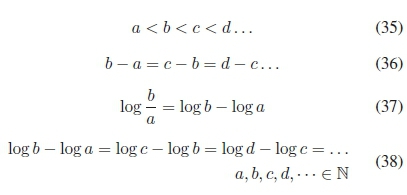
resulting in Stevens' new scales shown as a logarithmic interval scale.

The two main ideas are: The greater the stimulus the greater the JND i.e. when students are confronted with new knowledge or skills that differ greatly from their current knowledge and skill set, the less they are able to discern the details. The second is a method to transform ordinal scale elements into rational scale elements. These are further explored in the next section.

In two separate articles, Psychophysical analysis and A law of comparative judgment, Thurstone [28] [29] proposes a method to determine the JND. Starting from the assumption that a stimulus as described by Weber and Fechner leads to psychological values of psychophysics that he referred to as discriminal processes. To quote Thurstone [28, 369]:

"The psychophysical problem concerns, then, the association between a stimulus series and the discrim-inal processes with which the organism differentiates the stimuli."

Extending Thurstone [28] with the calculation of the probability of K > A,P(K >A):

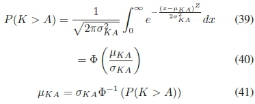
This is Thurstone's Law of comparative judgment with:

 

 

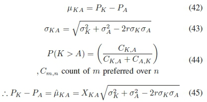
Equation (45) is called the observation equation, also referred to as the process equation.

In conclusion, Thurstone's Law can be used to estimate the just noticeable difference (JND) values for five or more observable events, mapped onto similar ordered and scalable processes under certain assumptions. For comparative method analysis examples see Tsukida & Gupta [30].

B. The Guttman Scale

Guttman [15] [16] developed a scale theory on which scales like the Beaufort wind force scale is based. It is accepted in principal that, for these scales, each higher scale value includes or implies all the ones below e.g. if one can add 3-digit numbers one can also add 2-digit and 1-digit numbers. While scoring event responses, event responses are ordered from those events that are scored lower to those that are scored higher or vice versa. A scale y is a simple function on event x i.e. a mapping between the original event being observed and its scale value after evaluation, Table VII.

 

 

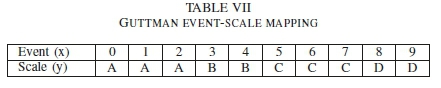
Unlike the mappings used by Thurstone, Guttman does not allow for event x mapping to be more than one y-value on the scale i.e. for the example above x = 0,1, 2 maps to y = A .

Guttman [15] suggests that a set of dichotomous attributes or evaluations is both necessary and sufficient as expression of simple functions for a single quantitative scale value or variable. When comparing two dichotomous items one can use a contingency table to measure the relations between items. This method was proposed by Pearson [23] in his 1904 paper. An example Guttman sequence or vector for a system containing anomalies is given as:

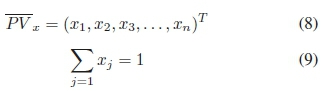
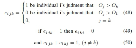
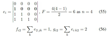
For n objects or events to be evaluated, let:

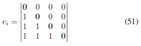
denote these objects. An experiment consists of N individuals that will be comparing the objects at hand by comparing them two at a time i.e. individual i is to judge object Oj to be lower or higher in value than object O_k,i = 1, 2, 3,....,Nandj, k = 1,2,3,...,n. Thus an experiment consists of a total of N χ n(n - 1)/2 comparisons. If each judgment consists of two judgements then there are N χ n(n - 1) judgements. Furthermore, let:

This means that every comparison of two judgements results in a total sum of one. The judgements of individual i are captured in a matrix form:

For an object Oj, let fj be the number of objects individual i judged to be lower than Oj, and let be the number of objects individual i judged to be higher than Oj. Then:

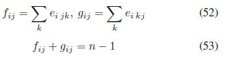
If F is the total number of comparisons, then:

Thus for our example:

If c is the number of times that object Oj was judged in the total experiment, and C is the total number of judgment within the experiment, then:

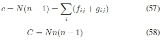
with each comparison consisting of two judgements.

Guttman's mean and variance for an experiment are presented next. Assume Xj is a variable that we must derive from our experiment for object Oj based on the comparisons, then the following variables are relevant.

For x-values of objects ranked higher than others by individual i, we have:

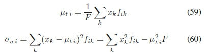
For x-values of objects ranked lower than others by individual i, we have:

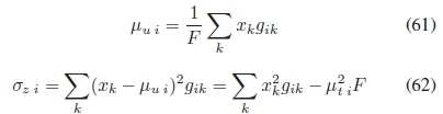
For V the mean of all x-values and W the total sum of the squares of the deviations from their mean of the x-values for the experiment, we have

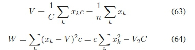
We defined two more variables, R the sum of squares between individuals and S the sum of squares within individuals:

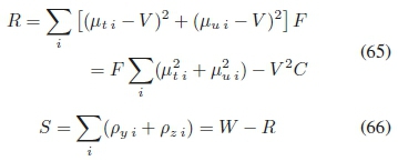
The correlation ratio is therefore:

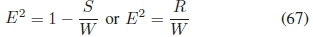
Thus the problem reduces to determining the set X of Xj that will minimize E². With E² being invariant to translations of the x-values we can set V = 0:

Taking the derivative of E²above with respect to X , we have:

also:

and:

Let:

Substituting we now have:

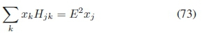
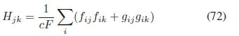
For x a row vector of the n elements Xj, and H a n χ n symmetric matrix

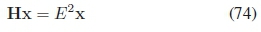
where x is the latent vector and E²is the latent root of H.

In conclusion, a scale is derived where any element observed higher on the scale implies all the elements lower on the scale i.e. the mastery of multiplication follows on the mastery of addition and subtraction.

C. The Analytic Hierarchy Process (AHP)

In their book, Saaty and Vargas [24] describe decisionmaking with the Analytic Hierarchy Process (AHP). The AHP is used in decision-making problems using a finite number of alternatives:

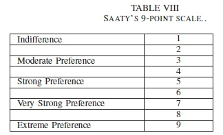
The scale Saaty and Vargas [24] used was a scale between 1 and 9, Table VIII.

 

 

This is based on a typical Likert categorical item. Given a set of alternatives the observer, or decision maker, is expected to provide a weight vector:

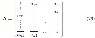
Formally the pair-wise comparisons are collated into a pair-wise comparison matrix A:

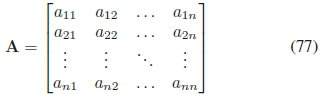
with the degree of preference of 2¾ to xj. More formally, Saaty and Vargas [24] suggests a ratio scale between weights:

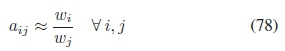
so we have:

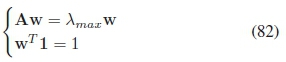
From linear algebra we can

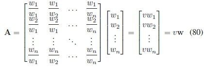
with v the eigenvalue and w the eigenvector of A. This relates to the work of Guttman above. The eigenvector can be calculated using the Perron-Frobenius method or the Geometric Mean method.

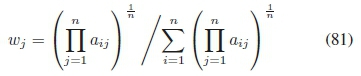
Due to the nature of this matrix, in its perfect form it has a rank of 1. Thus all the eigenvalues are 0 except for one. More over the eigenvalue for the perfect matrix is equal to n as the sum of the diagonal is equal to the sum of the eigenvalues for the matrix.

Thus we have:

In conclusion, the analytic hierarchy process is a method used to assist decision making by utilising comparative judgments and transforming them into priority vectors. The priority vectors are relative scales that have several interpretations. In this study they were used to set priorities and time schedules.

D. Competency Levels

The Dreyfus brothers, Dreyfus and Dreyfus [10], in 1980 published a paper on the five stages of learning. Their model stemmed from earlier works by Wason 1966 and Johnson-Laird, Legrenzi and Legrenzi 1972. In their work, Johnson-Laird et al [18], described a mental reasoning experiment in which they determined that participants found it easier to successfully execute the tasks of the experiment when it was in close relation to that which was familiar to them than if it was totally unfamiliar to them.

The five-stage model of Dreyfus and Dreyfus [10] consists of the following stages:

Novice - a person that can recognise non-situational context-free features and under supervision can apply a set of rules that govern the persons' actions based on these features

- Behaviourism;

Competence - With a lot of practice a person is able to recognise recurrent situational patterns referred to as aspects. A person now acts according to principles formulated by the instructor in accordance to the observed aspects i.e. the following of guidelines and treating all aspects as equally important;

Proficient - With continued practice a person is exposed to whole situations. These whole situations now start to expose meaning in terms of their relevance to achievements of long-term objectives i.e. the importance of aspects are aligned with their relevance to these objectives. In the words of Dreyfus and Dreyfus "Given a set of aspects and their saliencies, the performer uses a memorized principle which we call a maxim to determine the appropriate action" - Scaffolding;

Expert - At this stage a person can perform an action without following an analytic approach using rules, guidelines or maxims. The appropriate action response follows intuitively - Metacognition;

Mastery - A person that does not rely on principles but can produce an appropriate response almost instantaneously based on the person's current perspective.

In the 1970's Burch [5], an employee at Gordon Training International, developed an outline for Four Stages of Competency or learning a new skill. The four stages are labelled as:

Unconscious incompetent - A person knows, believes it to be true, an erroneous method to a situation and steadfastly insists it is correct;

Conscious incompetent - A person realises that they do not know the method to the situation;

Conscious competent - A person knows the correct method and can perform it with focused attention; and Unconscious competent - A person knows the correct method and can perform it fluently without much attention (it has become second nature).

The essence being, that one cannot know that which one does not know and only once one has reached a level of proficiency can one start to evaluate oneself or others.

These theories were tested in small example software applications using spreadsheets, Scilab or C++ before expansion and further development. The theories were then combined into a fully integrated demonstration application using C++ and the Windows application programming interface (Windows API).
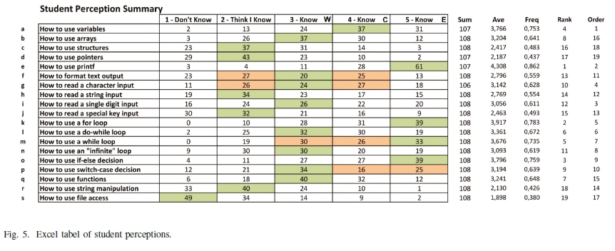
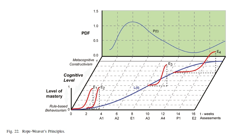