


Services on Demand
Article
 English (pdf)
 Article in xml format
 Article references
Indicators

Related links
-
 Cited by Google
 -
 Similars in Google
Share

 Permalink
SAIEE Africa Research Journal
On-line version ISSN 1991-1696
Print version ISSN 0038-2221
SAIEE ARJ vol.110 n.3 Observatory, Johannesburg Sep. 2019
ARTICLES
Maximum Demand Comparison of Aggregated Load Profiles for Vertical and Horizontal EWHs Due to a Fixed Draw Event
Yu-Chieh J. Yen; Ken J. Nixon; Willie A. Cronje
School of Electrical and Information Engineering, University of Witwatersrand, Johannesburg, South Africa (e-mail: yu-chieh.yen@wits.ac.za, ken.nixon@wits.ac.za, willie.cronje@wits.ac.za )
ABSTRACT
This paper shows a comparison of the vertical and horizontal tank orientation and the associated maximum demands from synthesized aggregated load models for various grid scenarios. Aggregated load profiles are produced by replicating a 50 litre (50% capacity) draw event for a 100-litre dual-mountable electric water heater (EWH) for each orientation. A total of 416 load profiles are produced containing 208 sets of horizontal and vertical aggregated profiles for comparison. Two factors are varied, (1) total EWH population from 1 to 1 million in various increments and (2) peak time window for initiating EWH draws ranging from 1 to 12 hours, where a Gaussian distribution is applied to the times each EWH starts participating on the grid. The resulting aggregated load profiles show that EWHs in the vertical orientation produce a higher aggregated maximum demand whereas the horizontal orientation can have a much lower aggregated maximum demand to a ratio of 0.58. A maximum demand ratio Ph/Pv of 0.80 is determined for a scenario similar to normal grid operation for a peak time window of 4 hours. The significance of this work is to quantify the difference in maximum power demand of a population of EWHs due to tank orientations in a controlled simulated environment.
Keywords: Domestic hot water, electric water heater, power demand, load aggregation, tank orientation, electrical grid.
I. INTRODUCTION
Electric water heaters (EWHs) are considered to be one of the largest loads, approximately 33 - 50% of total household energy use, and are therefore targeted for demand-side management schemes when the electrical power grid is under stress [1]. There are approximately 5.4 million electric water heaters (EWHs) in operation in South Africa, which have an estimated contribution of 2.94 GW to the evening peak load on the grid [2].
The purpose of this paper is to determine the difference in aggregated power demand for a fixed draw event of 50 litre (50% capacity) on a 1001, 2 kW a dual-mountable electric water heater (EWH) in both orientations (vertical and horizontal). The intention of this paper is to note the difference in heat replacement of the thermostatically-controlled element and to show the effect of this when aggregating in a larger scale system with varying peak demand time windows. This will inform on how a tank in horizontal orientation will affect the aggregated load on the grid power and how it may be compared to the more commonly modelled vertical orientation. Since it is estimated that 95% of EWH units in South Africa are installed in the horizontal orientation, most vertically-orientated models cannot be applied for estimating the total EWH load on the South African power grid.
There have been a few studies performed on the difference in performance of an EWH in different orientations; but these mostly focus on the effect of standing losses, which account for the energy storage capabilities of the system. McNeil and co-authors conducted a study on the cost-effectiveness of increasing thermal insulation and performs some measured comparisons of vertical and horizontal orientation with a focus on the standing loss differences [3]. Yen and co-authors measured standing losses on an EWH in vertical and horizontal orientation with different thicknesses of thermal insulation and concluded that horizontal orientation has a higher standing loss of up to 33.5% [4]. Delport examines the efficiency of an EWH through geometric mathematics to show that the water beneath the element will not get heated, concluding that horizontal is less efficient than vertical based on element location [5]. These studies investigate the difference in accumulated energy of the system, but do not consider the power demand due to a draw event and what effect it may have on the electrical power grid.
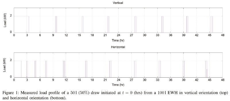
When considering the load power demand due to a draw event from an EWH in each orientation, there is a notable difference in the way the element replaces heat in the system. This is shown in Figure 1 which presents the measured element operations for the energy replacement after a 50 l draw event in vertical (top) and horizontal orientation (bottom) with subsequent standing loss operations up to 48 hours. While the total accumulated energy balances over time, the key difference between the profiles is the load demand i.e. the ON and OFF events and associated times of the element that replace heat hot water drawn from the tank.
In the vertical orientation shown in Figure 1, the element switches to ON state for one element cycle to replace the heat from the hot water drawn and then the tank enters steady-state at around t = 9 (hr) with a short, steady-state element event. The seven steady-state cycles in the vertical trace are evenly distributed in time, which shows that it takes only one element cycle to replenish drawn heat in the vertical orientation.
In the horizontal orientation shown in Figure 1, the element switches to ON state until t =1.5 (hr) with three subsequent short element operations at around approximately t =3(hr), t = 5 (hr) and t = 7 (hr). Finally, steady-state is reached at around t = 12 (hr). This difference in heat replacement pattern becomes relevant when aggregating loads for the grid consideration, in particular, the associated maximum demand. It should be noted that this heat replacement pattern has not been replicated in models in the literature.
Theoretical EWH models often predict the heat replacement requirements from a draw event in a single element operation much like element trace shown in the vertical orientation in Figure 1. The most simple models make the assumption that the tank holds a homogeneous temperature and predicts the amount of heat that needs to be replaced in the system and calculated the amount of time the element needs to operate in a single operation [6]-[9]. More complex models that take into consideration the stratification that occurs during a draw event are modelled as bi-nodal models; separating the tank into two regions, one hot and one cold [10], [11]. Nel and coauthors take a horizontal tank into account using a bi-nodal model [11]. The bi-nodal model also predicts the amount of heat that needs to be replaced in the system and calculated the amount of time the element needs to operate in a single operation.
Any EWH model that replaces heat due to a draw event in a single element operation is representative of a vertically oriented EWH. Horizontal EWHs replace heat in the tank in several element cycles, which literature does not represent correctly. While this paper does not develop either of these models, it aims to quantify the effect of demand predictions if loads are aggregated and show that there is a need for a representative horizontal EWH load model. Section II introduces concepts and terminology used in this paper. Section III presents the methodology used to aggregate the load profiles of a vertical and horizontal EWH element trace. Aggregation results are presented in Section TV where maximum demand ratios are compared and discussed in Section V. Finally concluding remarks are presented in Section VI.
II. Background
An EWH is a service device that supplies a user with hot water and in performing this function, results in power demand from the electrical power grid. As hot water is drawn by the user, indicated by flow, Q, the EWH needs to replace the energy drawn from the system with its fixed power rated element, P, over a period of time, which results in power demand on the grid. The states causing power demand events are discussed further in Section II-A.
With many other users and EWHs interacting with the national power grid, the effects of each load or power demand event can be aggregated to a load profile that could be analysed for demand-response schemes; which is discussed further in Section II-B. This is analysed using a technique called load diversity, which is discussed further in Section II-D.
A. States of Electric Water Heaters
Electric water heaters (EWHs) operate the temperature around a preset hysteresis set-point. The thermostatically-controlled states of a typical EWH (in vertical orientation) are shown in Figure 2. The EWH loses heat to the environment through its built-in insulation (cooling state, C), and when the temperature at the thermostat reaches a lower bound, TL, the element switches to ON state (heating state, H) to heat the tank to an upper bound temperature, TH. This is steady-state operation (S) of the EWH, which is usually characterised as a heating state event with a short duration. Larger element events occur when hot water is drawn from the system (draw state while element is operating, D, £(1)), and the element is in the ON state for longer to heat inlet temperature water up to its set-point.

When the element switches to ON state to reheat the whole tank to the upper set-point, this results in load demand that draws from the electric grid. Since the element has a fixed power rating, the amount of time the element operates defines the replacement energy to the system. Steady-state replacement events usually operate for short periods of time (in the range of minutes) and are separated by long periods (in the range of hours), depending on thermal insulation of the system and the ambient temperature. Element events due to hot water draws can vary in length of time due to the volume drawn (and tank orientation, as will be shown later), but are usually larger than steady-state events.
B. Load Aggregation
Load aggregation is a technique used to determine the load contribution of an individual device or unit within a greater population of concurrently operating devices. The total summation of power demand from each unit over each time step within an operational period (usually 24-hours) results in an aggregated load profile. The time of day that the unit uses power becomes relevant in a 24-hour load profile where large interconnected systems are considered, especially with the requirement of power utilities to supply power against the demand, such as on an electrical grid application.
For the purposes of this investigation, real-time or realistic hot-water draw times with variable draw capacities are not considered for the production of the load profiles in the discussion. The focus is to compare aggregated maximum demand based on tank orientation. The EWH population will be varied to determine the effect it has on the maximum demand when comparing orientations. In addition, the times that each EWH starts participating on the grid is determined by a normal distribution with an upper and lower bound defined, to simulate the effects during peak load times.
C. Maximum Power Demand
The maximum power demand from an aggregated load profile, PAgg , is when the total loading on the system reaches a maximum value. This happens when the most number of EWHs are in ON state in the measured time frame. The maximum power demand is associated with a specific time and also indicates the maximum power that a grid needs to supply.

where
PAggthe maximum demand in time range,
L is a contributing load,
Ρ is a power value of load when ON (kW),
i is the load iterator,
n is the total number of loads in the system.
In the context of this paper, the maximum demand in the load profiles produced by a vertical EWH is denoted, PAggvand maximum demand in the load profiles produced by a horizontal EWH is denoted, PAggH. A ratio of the two quantities  is determine to compare the difference in maximum demand.
D. Load Diversity
Load diversity on a system is quantified by the load factor, which is the probability of equipment coincidentally switching into ON state with another piece of equipment.

where
fdiversitythe load diversity factor at a specific time,
L is a contributing load,
i is the load iterator,
n is the total number of loads in the system.
This term is used to analyse the difference in resulting load profiles and is used to express the times when the system can experience stress. High load diversity indicates when a larger number of devices are drawing load at a specified time frame, which indicates when the power grid needs to supply higher loads.
III. Methodology
This section presents a comparison of the simulated aggregated effects for a partial draw event of a tank in vertical and horizontal orientation. The EWH used in this study is a 100-litre storage tank with a 2kW element. The element data obtained for this study was measured from a real draw event at 6 l/min flow rate, with a 50 litre (or 50% of the total tank capacity) in each orientation under lab conditions. This volume of hot water draw is chosen to simulate a low flow bath or shower, which according to ASHRAE, is around 571 [12]. The hot water draw results in an set of measured load profile of element operations, which differ based on tank orientation. One set of element trace measurements is taken for the tank in each orientation as discussed in Figure 1 in Section I. Both tests are performed in the same season with similar ambient temperatures. The measurements are sampled at a second resolution.
The load aggregation is achieved through the replication of the measured signal for each participating EWH with a variable delay. The benefit of limiting the aggregation to one set of measured element traces for a fixed draw is to determine the effect of other factor that come into play in aggregated Systems, EWH population and peak time windows for EWH participation.
A. Simulated events for aggregation
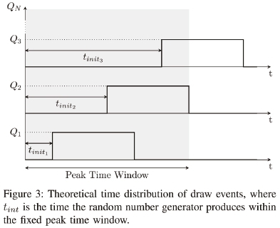
Using measured element data from a single 50 litre draw event in each orientation from Figure 1, the aggregated load demand is determined through the replication of the original signal in a number of different configurations. There are two variables that are controlled: EWH population and the peak time window. The EWH population is the number of EWHs participating on the grid during that period, which will be limited to a single 50 litre draw with steady-state operations thereafter. The varying population for EWHs is selected from 1 to 1 million EWHs in a range of [1; 2; 4; 8; 10; 20;...; 1,000;...; 1,000,000] resulting in 16 variations. The second controlled variable is the peak time window, which is the time interval that each EWH starts to participate on the grid based on the randomly generated value, as shown in Figure 3. This allows for variability on the system and simulates when hot water demand would occur in a specified peak time window, ranging from 0 hours to 12 hours in one-hour intervals.
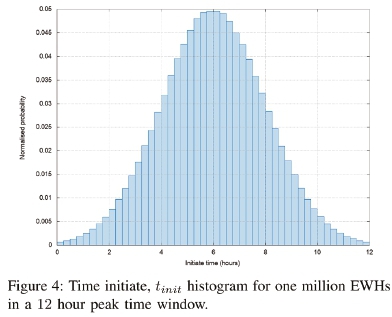
The time that each EWH starts to load the grid, tinit, with a draw event heat replacement is determined by a random number generator that has a Gaussian distribution [13]. The time produced from the random number generator is within the range of the peak time window, as shown in Figure 3. The Gaussian distribution is used in an attempt to model human behaviour and to produce definitive regions for maximum demand for ease of comparison. Figure 4 shows the normalised probability distribution used for a 12-hour time frame for the one million EWH population. The same initiated time is applied to each paired load profile for vertical and horizontal simulation. And finally, each EWH only participates on the grid when its draw is initiated, therefore steady-state operation before that time is ignored.
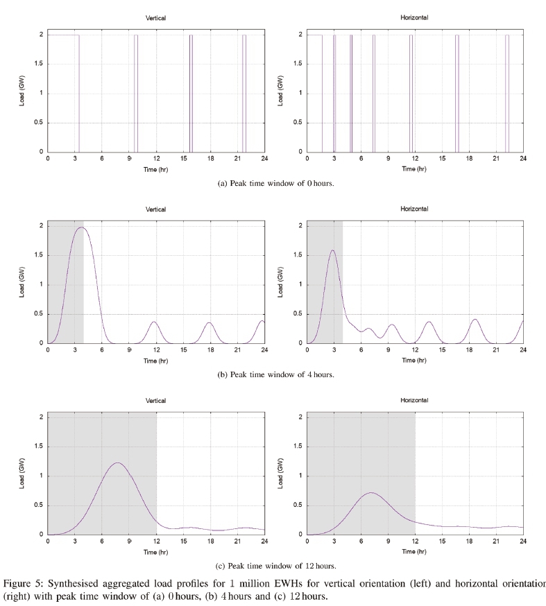
There are 208 sets of load profile simulations that are run for each orientation (16 different EWH populations and 13 time frames), which results in a total of 416 load profiles. Three different peak time windows examples at 0, 4 and 12 hours are presented for 1 million EWHs in Figure 5 (a), Figure 5 (b) and Figure 5 (c) for side-by-side comparison. The population of 1 million EWH is chosen as it shows the scaled trends and is therefore more comparable to large power grids. Smaller populations show much more variation in the demand profile and is difficult to make conclusive statements.
Each set of load profiles shows the synthesised power demand from EWHs in the vertical and horizontal orientation with identical hot water service demand of fixed hot water load of 50 litre, fixed temperature and the same randomised seed for time of initiated draw. In each figure, the peak time windows are shaded in grey, which coincide with the maximum demand in each case.
1) 0-hour Time-Window: This is chosen as a baseline measurement to show the effect of all 1 million EWHs initiating draw events at the same time, shown in Figure 5 (a), which results in the original element pattern with a demand that is multiplied by the EWH population; which is intuitive if all EWHs operate at the exact same time. Since there is no variation in the times of initiation, the instances of power demand are all at the same loading of 2GW, diversity is maximised to a factor of 1 and therefore, this shows the worst-case scenario for the grid. Here, the maximum aggregated power demand for each orientation are identical.
2) 4-hour Time-Window: This time frame comparison shown in Figure 5 (b) has some similarity to real peak periods on the South African power grid, which occurs from 17:00-21:00. In this situation, the vertical orientation still has a maximum aggregated power demand of 1.98 GW, which is close to the system maximum of 2 GW, whereas the horizontal orientation has a smaller maximum aggregated power demand of 1.60 GW. Therefore, the horizontal maximum demand is only 0.80 of the vertical peak (PAggH / PAggv)- The demand increases again at t = 7(hr) in the horizontal orientation, which results from the subsequent element operations that occur from a draw event in the horizontal orientation. Thereafter, steady-state peaks are observed. For both vertical and horizontal, the steady-state peaks are minor peaks that do not overlap.
3) 12-hour Time-Window: This time frame comparison shown in Figure 5 (c) shows the same population of a million EWHs with a much larger peak time window to initiate draw events. This results in much lower maximum demand in both orientations, with the maximum aggregated power demand for vertical at 1.23 GW and that of horizontal orientation of 0.72 GW. Therefore, the horizontal maximum demand is only 0.58 of the vertical maximum demand. The aggregated demand from the steady-state operations are almost indistinguishable from each other, tending towards a constant demand. This is a scenario that will likely not happen on the South African grid, as peak demand times frames are usually much shorter than 12 hours. However, this would be considered the ideal scenario for a grid operator.
IV. Aggregation Results
The key feature from each of the load profiles is the maximum demand and for this study in particular, the comparison of maximum demand based on tank orientation for the same level of hot water service. Therefore, a ratio of PAggH /PAggv
is used to describe the comparison of peaks, where Ρα99η is the maximum demand for the horizontal orientation, and PAggvis the maximum demand for the vertical orientation, as defined in Section II-C. The variations in these ratios are discussed against the two controlled variables: EWH population and the peak time window. In cases where PAggH/PAggv= 1, the demand peaks of both orientations are equal. This can also be expressed as a ratio of load diversity factors, fdiversityat the peak time, as defined in Equation 2.
A. Demand Ratio Against EWH Population
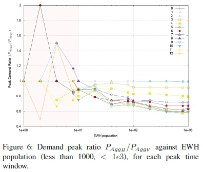
The resulting demand ratios are plotted against the EWH population for each peak time window in Figure 6. The trends are plotted on a log scale (base 10) on the x-axis to account for the large EWH populations considered. For an EWH population of less than 10 (or 1e1), as depicted in the shaded region in Figure 6, there is no discernible pattern that can be observed for the ratio of PAggH /PAggv; in some cases PAggH is greater than PAggv. For EWH populations larger than 1θ, the ratio becomes more stable and PAggvis consistently greater than PAggH, which produces a ratio of a range [0:1].
The load profiles with demand ratios of lower than unity are presented in Figure 7, for EWH populations of 10 (or 1e1) up to 1 million (1e6). The peak time windows are chosen in the plot to show general trends; some have been intentionally omitted for visual clarity. There is some variability in the earlier samples (EWH populations up to 1, 000 (or 1e3), and thereafter, the ratios become constant for the population sample. At the far right end of the graph at EWH population of 1 million (or 1e6), the demand ratios for chosen samples at peak time windows of 0, 4 and 12 hours can be determined from the discussion of Figure 5 (a), Figure 5 (b) and Figure 5 (c). This shows that in the extreme case of 1 million EWHs participating on the grid with a peak time window of 12 hours, there could be a lower-bound difference between horizontal to vertical by a factor of 0.58 for the maximum demand. For a more realistic peak time window of 4 hours, there could be a lower-bound difference between horizontal to vertical by a factor of 0.8 for the maximum demand.
B. Maximum Demand Ratio Against Peak Time Window
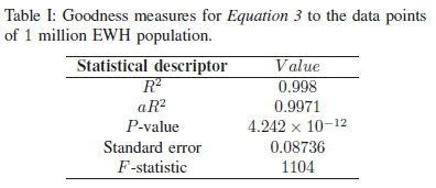
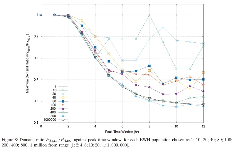
The demand ratios plotted against the peak time window are presented in Figure 8. Again, the trends for varying EWH populations are chosen for visual clarity; the jump from 800 EWH to 1 million EWH shows that there is convergence of the trends. The ratios are close to unity for peak time windows of 0, 1 and 2 hours; with larger time frames, it can be seen that a larger mismatch of peaks occurs. This could be a factor of the initial replacement element cycles that are roughly 3 hours for vertical and 2 hours for horizontal. Once again, trends for lower EWH populations exhibit randomness (10 and 20 shown in the graph; 2, 4, 8 omitted). In this graph, it clearly shows that from a population of 800 up to 1 million EWHs have ratios that remain constant. As a function of peak time window, the resulting ratios follow a smooth decay function that can be described using Equation 3. The "goodness" measures for Equation 3 are presented in Table I, which indicates a good match to the dataset for a population of 1 million EWH.

V. Discussion
From the load profile examples presented in Figure 5 (a), Figure 5 (b), Figure 5 (c) for the same draw capacity in vertical and horizontal orientation, it is evident that the vertical demand is generally higher and more predictable whereas the EWH in horizontal orientation lower peaks and has a secondary peak due to its subsequent element operations to replace drawn energy. The difference in the time interval of usage patterns also has an effect; the smaller the intervals between usage events, the higher the maximum demand, as more elements switch into ON state at the same time to draw energy from the system. The larger the intervals between the usage events shows a lower overall maximum demand which is easier for a grid utilities to manage. It should be noted that the same total volume of serviced hot water is produced and approximately the same energy is used to replace the drawn energy.
From the compared peak ratios, PAggH/PAggv, presented with varying EWH populations, it has been shown that ratios are random with EWH populations of below 10, are consistently less than or equal to one for EWH populations above 10 and stabilise at EWH populations greater than 1,000. From the compared maximum demand ratios, PAggH/PAggv, presented with varying peak time windows, it has been shown that a unity ratio coincides with the times of the initial element event for energy replacement. The change in ratio follows a smooth decaying function and EWH populations larger than 800 tend towards the function.
VI. Conclusion
This paper has produced load profiles for vertical and horizontal EWHs that illustrates significantly different maximum demand values that loads the grid. This is shown from controlled environment simulations with a fixed 501 draw event. When these differences in load demand are aggregated over a 24-hour profile, it is shown that there is a significant difference between tank orientations in contribution to the maximum demand and diversity on the power grid. Greater EWH populations and larger draw peak time windows exaggerate the differences and indicate a much lower aggregated peak (with a lower bound of 0.58). For a more realistic peak time window of 4 hours, the ratio of maximum demand is in the order of 0.8. This means that conventional EWH models that usually describe the heat replacement of a vertical EWH with a single element operation could overestimate maximum load for a grid that has a EWH population that is primarily horizontally oriented.
If the maximum load demand for South African horizontal EWHs is to be fully understood, a thermostatically-controlled model of a tank in horizontal needs to be developed, which correctly the multiple ON/OFF cycles of the element in heat replacement after a draw event. Since most published EWH models for aggregation purposes replace heat in one element cycle (remnant of vertical orientation), this study has identified a requirement for a model in horizontal orientation that correctly traces the many ON/OFF cycles that characterises heat replacement observed in this orientation.
The paper has provided a framework for comparing maximum demand in aggregated systems. This aggregation model could be extended to vary the number of vertical and horizontal EWHs to estimate a realistic load profile on the South African grid. With a sufficient horizontal element model, this framework could also be used for varying draw volumes and flow rates.
References
[1] O. M. Popoola and C. Burnier, "Solar water heater contribution to energy savings in higher education institutions : Impact analysis," Journal of Energy in Southern Africa, vol. 25, no. 1, pp. 51-58, 2014. [ Links ]
[2] Eskom, "1317 geyser fact sheet," http://www.eskom.co.za/sites/IDM/Documents/1317_geyser_fact_sheet_no_rmr.pdf, 2013, [Online; accessed 2015-10-28].
[3] M. McNeil, T. Covary, and J. Vermeulen, "South Africa Geyser: Cost-Effectiveness Study of Increased Insulation," in Super-Efficient Appliance and Equipment Deployment Programme (SEAD), South Africa's S&L Programme, 2014.
[4] Y.-C. J. Yen, K. J. Nixon, and W. A. Cronje, "Experimental results of energy usage for an electric water heater in vertical and horizontal orientation under steady-state conditions," in South African Universities Power Engineering Conference (SAUPEC), Stellenbosch, South Africa, 2017, pp. 707-712.
[5] G. J. Delport, "The geyser gadgets that work/do not work," in Domestic Use ofEnergy, 2005.
[6] P. S. Dolan, M. H. Nehrir, and V. Gerez, "Development of a Monte Carlo based aggregate model for residential electric water heater loads," Electric Power Systems Research, vol. 36, no. 1, pp. 29-35, 1996. [ Links ]
[7] N. Lu, D. P. Chassin, and S. E. Widergren, "Modeling uncertainties in aggregated thermostatically controlled loads using a state queueing model," IEEE Transactions on Power Systems, vol. 20, no. 2, pp. 725733, 2005. [ Links ]
[8] P. Palensky, F. Kupzog, A. A. Zaidi, and K. Zhou, "Modeling domestic housing loads for demand response," in Proceedings - 34th Annual Conference of the IEEE Industrial Electronics Society, IECON 2008, 2008, pp. 2742-2747.
[9] H. Hao, B. M. Sanandaji, K. Poolla, and T. L. Vincent, "Aggregate flexibility of thermostatically controlled loads," IEEE Transactions on Power Systems, vol. 30, no. 1, pp. 189-198, 2015. [ Links ]
[10] J. Kondoh, N. Lu, and D. J. Hammerstrom, "An evaluation of the water heater load potential for providing regulation service," IEEE Transactions on Power Systems, vol. 26, no. 3, pp. 1309-1316, 2011. [ Links ]
[11] P. Nel, M. Booysen, and A. van der Merwe, "A computationally inexpensive energy model for horizontal electric water heaters with scheduling," IEEE Transactions on Smart Grid, vol. 9, no. 1, 2016. [ Links ]
[12] ASHRAE, "2003 ASHRAE Applications Handbook (SI)," American Society of Heating, Refrigerating and Air-Conditioning Engineers, 2003. [Online]. Available: ashrae.org
[13] G. Marsaglia and W. W. Tsang, "The ziggurat method for generating random variables," Journal ofStatistical Software, Articles, vol. 5, no. 8, pp. 1-7, 2000. [Online]. Available: https://www.jstatsoft.org/v005/i08 [ Links ]
Manuscript received June, 1, 2018
revised January 15, 2019

Yu-Chieh J. Yen was born in Taipei, Taiwan. She received her Bachelor of Science in Electrical Engineering from the University of the Witwatersrand, Johannesburg in 2008. She became an associate lecturer at the same institution in 2010 and subsequently received her Master of Science in Engineering in 2012. In 2013, she became a lecturer at the university. She started her Doctor of Philosophy in 2014 where her research interests lie in energy systems with a focus on load modelling and hot water systems.

Ken J. Nixon was born in Johannesburg, South Africa in 1974. He received a BSc(Eng) degree in electrical engineering in 1996, an MSc degree in engineering in 1999 and a PhD degree in 2006, all from the University of the Witwatersrand, Johannesburg South Africa.
From 2001 to 2005, he was a Lecturer, and from 2006 to 2011, he was a Senior Lecturer with the School of Electrical and Information Engineering. Since 2012, he has been an Associate Professor with the School of Electrical and Information Engineering, University of the Witwatersrand, Johannesburg, South Africa. His research interests include high voltage engineering, earthing and lightning protection, high performance computing, software engineering, applied machine learning and the sustainable use of energy.
Prof. Nixon became a Member of the SAIEE in 2002, a Senior Member in 2007, and was elected as a Fellow in 2012. He served as a member of the SAIEE Council from 2007 to 2013. He has been a Member of the IEEE since 2005. He was the recipient of the SAIEE Keith Plowden Young Achievers Award for his commitment to education at secondary and tertiary levels p,articularly in electrical engineering in 2008.

Willie A. Cronje graduated with his B.Ing in Electrical Engineering from the Rand Afrikaans University, in Johannesburg, South Africa, in 1985. He subsequently graduated with his M.Ing in 1987 and D.Ing in 1993 from the same institution. He was a staff member at the institution before joining the University of the Witwatersrand as holder of the Mondi Chair on Machines and Drives in 2004 and headed the machines research group. He subsequently changed his research interest to renewable energy systems and has held the Alstom Chair in Clean Energy Systems Technology from 2013 to 2018.
This work is based on the research supported in part by the Alstom Chair for Clean Energy Systems Technology (ACCEST), the National Research Foundation of South Africa (unique grant no: 98241), and the Department of Higher Education and Training (DHET).

