ARTICLES

 

Distribution Pole Monitoring Using Magnetic Field Characterization

 

 

Jason Hardy^I; Edward Boje^II

^IWas with the Department of Electrical Engineering, University of Cape Town, Rondebosh, Cape Town 7700, South Africa e-mail: HRDJAS001@myuct.ac.za
^IIWas with the Department of Electrical Engineering, University of Cape Town, Rondebosh, Cape Town 7700, South Africa e-mail: edward.boje@uct.ac.za

 

 

---

ABSTRACT

This paper outlines methodologies for monitoring the supporting structures of distribution power lines by characterizing the rotating magnetic field established by the current carrying conductors. This is achievable since the resultant magnetic field is a function of phase currents and pole geometry. The resultant magnetic field vector (measured using 3-axis magnetic field sensors) rotates with time and forms an ellipse. The formation of an ellipse provides an expedient mechanism for data compression and comparison between pole geometries, which is achieved by wireless communication between two adjacent poles. A detected change in geometric state between poles can be sent to the substation at the end of the line. This data can be used to detect, locate, mitigate, prevent, or repair damage caused by a fallen power line. An experiment was performed to demonstrate the working principal of the single-sensor design methodology. A prototype instrument is under development to be field tested. A simulation was performed to show the effects that nearby metal structures have on the resultant magnetic field. The solution is realizable through the low-cost implementation of existing technologies and practices. A preliminary version of this paper was presented at the South African Universities Power Engineering Conference, SAUPEC 2018.

Keywords: distribution pole monitoring, magnetic field, MEMS sensor.

---

 

 

I. INTRODUCTION

Worldwide, there are hundreds of millions of wood poles supporting distribution lines. For example, in the United States there are over 10 million km of distribution power lines [1], while Eskom operates around 300 000 km of overhead distribution lines energized at 22 kV or lower [2]. These lines are typically supported by wooden structures (poles) with a height of approximately 8 m, spaced no further apart than 200 m [3]. Therefore, under Eskom's responsibility alone (i.e. not counting 3rd-party installations and municipality distribution networks) there are over 1 million poles. Depending on the environment, the lifespan of wooden poles is around 40 years before they succumb to groundline decay, and fungal or insect attack. Moves to ban pesticide treatment of wood poles will tend to shorten field life. Early failure occurs due to unpredictable weather or human activity (strong winds, lightning, fire, car accidents, etc.) [4], [5], [6], [7]. Apart from the threat to public safety, falling power lines cause financial loss to the utility as a result of damage to property, fire, loss of sales and lost opportunity due to interrupted power delivery [8]. The risks and financial loss can be mitigated by appropriate maintenance and fast, accurate fault reporting. Current methods of inspecting distribution lines and supporting structures are costly, labor intensive and constrained by legislation (helicopters, drones, walking the line) [9]. Previous work has been done for an Internet of Things (IoT) solution using different sensing and data transmission techniques [10], [11].

A. Proposed Solution

An economically viable solution is sought to minimize (or mitigate) the damage caused by fallen power lines. The method proposed is to design a sensor which is able to detect physical changes associated with various failure modes and report these back to the substation for appropriate further action. These sensors are to be installed ubiquitously along the power line to provide specific and localized information about the failure (which particular pole or line has fallen). They will operate as a Low Power Wide Area Network (LPWAN).

1) Low-cost: The key to the success of the proposed solution is a low-cost, mass producible design, with the underpinned "value-add" of saving money. With the advent of cheap Micro-Electro-Mechanical Systems (MEMS) sensors, it is possible (but not necessarily cost effective) to measure the pole orientation (using accelerometers), 3-axis magnetic field, temperature, pressure, and humidity at each pole. Measuring the electric field would be useful but this is problematic due to tracking on the pole due to moisture and pollution [10].

2) Magnetic field measurements: In order to reduce installation and production costs of such a device non-contact detection of current and voltage is desired [12], [10]. The problems associated with this are the indirect measurement of metrics, the reliability of readings, the sensitivity of apparatus required, as well as power supply. The current flowing in each phase can be determined by measuring the magnetic field established by the current carrying conductors and knowing the geometry.

3) Integration with current technology: The development of a device does not provide a complete solution; a system must be created to ensure that the utility receives all the necessary metrics, such that they can be interpreted and acted upon. As a result, the feasibility of such a product should be clearly seen in financial as well as technology terms. It is intended that the devices in the field will send their data to base-station devices, located in substations, which are able to give commands and status indicators via IEC 61850 protocol for the automation of switchgear. In the event of a malfunction an alert will be generated for the issue to be rectified and the line can be de-energized autonomously if required.

4) Power Source: An obvious power source is harvesting from the power line by means of a clamp-on current transformer. As discussed in Section II-A below, installing the device too close to the conductors may render magnetic field measurement techniques impossible, as readings are sensitive to environment geometry (Figure 1). Additionally, with magnetic field sensors placed close to one of the conductors, the field readings of the other phases might be dwarfed because of limited sensor turn-down. Another option is harvesting solar energy by means of a solar cell with a MPPT tracking charge controller. This approach gives easier (and hence cheaper) installation as the device can be installed outside of the "hot-zone", and more freedom in terms of device location.

 

 

II. MAGNETIC FIELD SENSOR DESIGN

Techniques of determining conductor behavior by analyzing magnetic fields have been developed [13], [14]. This technique relies on current carrying conductors establishing a magnetic field proportional to the current flowing through the conductor. For simple geometries, this is expressed in Biot-Savart's equation (1).

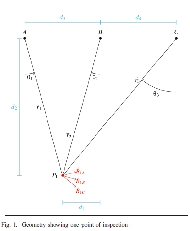
B is the magnitude of magnetic field tangential to the line, I is the magnitude of current flowing in a conductor, μ₀ is the permeability of free space, r is the distance between conductor and point of inspection. In order to optimize the usage of a magnetic field sensor, a representation of its physical placement is described. With [13] as a demonstration on a transmission line, a similar application can be envisaged for a distribution line use-case. It is common for 33 kV distribution lines to feed step-down transformers rated at 315 kVA and above. This implies that a current of 5.5 A per phase can be expected at full load. At a radial distance of 1 m, the rms magnetic field expected from a conductor carrying 5.5 A is 1.1 μT. A 3-axis magnetometer (MEMS sensor) can be placed at a known location (point of inspection) near the conductors to sample the magnetic field at known time intervals. These readings, in vector form, must be decomposed as to determine the individual contribution that each conductor gives to the magnetic field at the point of inspection. These contributions are visualized in Figure 1.

A. Geometry

Point of inspection P₁has a sensed magnetic field vector B₁ in the x-y plane orthogonal to the line (post-processing of the 3-axis magnetometer signals allows correction of sensor-to-line misalignment through a rotation so that there is no z axis component),

This magnetic field is established as a result of the 3-phase current flowing in the conductors A, B and C. It is clear that

Expanding:

Substituting (1), the following is produced.

(7) is well determined for finding the quadrature components of balanced line currents but we are interested in the general case.)

The conditioning of M₁ in (6) depends on the geometry which is fixed for a particular installation (unless there is a failure) but could be inaccurately known because field installation should ideally not require accurate site measurements of the physical environment, namely distances d₁to d₄ in Figure 1. The line currents cannot be determined from (6) as it is under-determined (M₁ in (6) has m< n). For this reason, a second point of inspection, P₂, is introduced as shown in Figure 2.

 

 

Provided that the geometry does not result in loss of rank, the pseudo-inverse can be taken to solve for 3-phase current components.

M in (8) is over-determined (m x n = 4 χ 3) but consistent in the absence of measurement noise and geometry errors. The least squares solution for current in each phase is found using the Moore-Penrose pseudo-inverse.

where the pseudo-inverse, , is defined as

Including a second sensor to monitor the 3 conductors increases the device cost, however, the current in each phase can be determined independently. The distance between the points of inspection P₁and P₂, namely d₁and d₂, affect the condition of matrix M, and the accuracy of the measurements taken. As mentioned in [13], with three sensors the condition of the matrix will be minimized if each sensor is placed directly below its corresponding conductor. The intersensor distance affects the production cost of the device as the further apart the sensors are, the higher the PCB and enclosure production cost. A cost-performance optimization will determine the appropriate spacing of the sensors. Figure 3 shows a simulation of the rotating magnetic field (ellipse) about various points of inspection underneath a 3-phase power line, with balanced 3-phase current. This illustrates that the ellipse formed at each inspection point has a unique characteristic depending on its position. These defining parameters are each ellipse's major axis scale a, minor axis scale b, and degree of rotation α. The strength of the magnetic field over one current cycle is proportional to the area of the ellipse.

 

 

By extracting the time varying components, (7) can be rewritten as

Assuming a balanced 3 phase current, known distances between conductors (d₃ and d₄ - determined by the design of the distribution pole cross-member), and known x offset of the sensor ((d₁+ d₂) - to be designed), it is hypothesized that a relationship can be drawn between d₅, \I\ and α, a, b, such that d₅ and \I\ can be solved given a data-set of points describing an ellipse. By removing the parameterization of time, (7) and (11) can be compared as the same ellipse in space. The values of α, a, b can be determined using the method of least squares on the data-set. If the device is aware of its precise location, it will be able to determine any mechanical failures (fault classification) based on a perceived change in geometry. This is described in [13], however using 3 sensors.

B. Practicality

The above procedure aims to address device practicality, since d5 will vary due to non-exact device installation on the upright member. This method is not limited to a horizontal conductor arrangement, as the governing principle relies on the radial distance and angle between (each) conductor and sensor, and not the position of one conductor relative to another.

C. Measurement Sensitivity

3-axis MEMS magnetometers (such as the MMC5883MA by MEMSIC) report a total rms noise of 0.04 μT[15]. This corresponds to a field resolution of 0.2 A at 1 m or to a distance resolution of 3.5 cm at 1 m and 5.5 A rms. Noise can be subsequently digitally suppressed. This implies that meaningful current measurements can be made, and that structural fault classification can be performed. An alternative to MEMS magnetometers are individual magneto-resistive Wheatstone bridge arrangements, which may provide a greater accuracy at the expense of additional circuitry (instrumentation amplifiers, ADC, etc.). This will increase the development time, and production cost of the device.

D. Fault Classification

Fault detection, isolation, and recovery (FDIR) adds to the economic value-add of the device. If the device is able to report specific details on the fault condition, a specialized team can be dispatched to rectify the issue. Additionally, this information can provide relevant data on how to reduce future occurrences. Some examples of distribution power line faults include fallen vertical support, detached conductors, and cross-member attachment point malfunction, resulting in an irregular angle of attachment. With the expected measurement sensitivity, it is conceivable that these changes in conductor geometry can be detected.

 

III. SINGLE SENSOR DESIGN

A qualitative investigation has been performed to determine if a change in pole and line geometry can be detected using a single magnetometer per pole, as a means to further drive down device cost. Given that the current flowing through the conductors supported by adjacent poles is identical, a change in magnetic field characteristic (ellipse) should be apparent at each pole sensor in the event of current fluctuations. Conversely, should there be a change in geometry in one of the poles, the magnetic field characteristic will only change for that pole and not adjacent poles. (12) and (13) represent two adjacent poles, with common current I, each generating their unique ellipse (B₁and B₂). Each pole has a unique geometry (M₁and M₂ with M₁ = M₂ for uniform pole and sensor configurations) determined by the arrangement of the conductors, and the installation of the device.

As in (11) the rotating magnetic field can be described as an ellipse with parameters a, b, α, such that B_n(a_n,b_n,a_n). These parameters can be wirelessly communicated between poles in order to determine whether a change in ellipse is common (due to change in current) or isolated (due to change in geometry). Factorizing the common current between both sensors, (12) and (13) can be reduced to

where ß_nis the orientation of the 3D readings with respect to the X-Y reference plane (see Section III-B).

A. Experiment set-up

A scaled 3-phase power line was constructed, with two 3-axis magnetometers placed near the conductors; each sensor representing a device on adjacent poles. This is shown in Figure 4.

 

 

B. Experiment procedure

A constant load was applied to the power line and the sensors began taking readings of the magnetic field. After a period of time, the magnetometer representing pole 1 was moved slightly, while keeping the geometry of pole 2 and the current constant.

In order to minimize the transmission of data stored and communicated, the magnetic field readings were reduced to their ellipse parameters. For the experiment this was performed off the microprocessor, but in practice will be implemented locally. The following procedure was adhered to[16], [17].

• 100 readings were captured, forming an ellipse in 3D.

• A plane of best fit for the ellipse was found.

• A rotation was applied to the ellipse in order for it to lie in a plane parallel to the X-Y reference plane. This angle of rotation shall be called β.

• The ellipse was flattened such that all values are co-planar.

• A curve-fitting by means of least-squares was performed on the ellipse in order to extract its parameters a, b, α.

• The above procedure was repeated 100 times for each sensor, yielding 100 sets of ellipse parameters per sensor.

C. Results and discussion

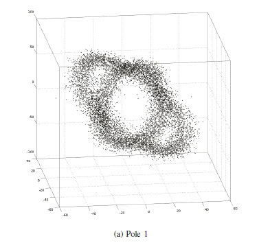
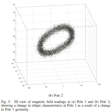
The magnetic field vectors (pre-processing) are shown in Figure 5. Figure 5(a) shows a change in ellipse for pole 1. Figure 5(b) shows no change in ellipse for pole 2. The distinction in change of state of the readings from pole 1 can be seen (post-processing) by analyzing the ellipse parameters.

 

 

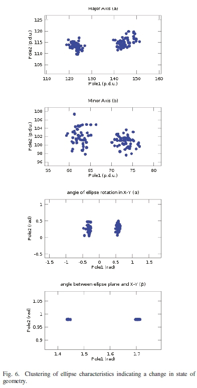
100 sets of ellipse parameters for each pole B ₁(a₁,b₁,a₁,ß₁) and B₂(a₂,b₂,α₂,β₂) were extracted from the recorded dataset following the procedure outlined in Section III-B. Each set was sampled over the same time interval for each pole.

Each ellipse parameter was plot separately, as shown in Figure 6. Each point in the subplot(s) represents a time interval of samples for the parameter in question. This shows the relationship between the ellipses formed by sensor 1 and sensor 2 in accordance with (14). Two clusters in each image can be seen, which represent two different states, namely before and after the movement of sensor 1. In this way, we are able to detect that there has been a change in geometry of pole 1. The data is clustered since the current was held constant. In the event of a changing current the data traces a locus with change in both axes (for example, a smaller current reduces the size of magnetic field, therefore area of ellipse, and size of axes a and/or b for both sensors).

 

 

 

IV. MAGNETIC FIELD SIMULATION

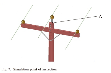
In order to observe and understand the nature of the instantiated magnetic field surrounding a power line, a finite element 3D modeling software ANSYS Maxwell was used. A particular area of interest is the effect of fixtures (such as galvanized steel bolts and struts) with a high magnetic permeability on the magnetic field. These fixtures may distort the magnetic field around the location of the device resulting in spurious measurements. A 3-phase delta-connected power line was modeled, and excited by a balanced current (120° separation between phases, 5A amplitude). The parameters of the structure are closely coupled to the design parameters as specified in [19], and can be seen in Figure 7.

 

 

A. Simulation procedure

A simulation was run featuring only the 3 conductors with their excitation currents, surrounded by air, without the magnetic permeability effects of any structural supporting components. This was performed to establish a well-predicted and acceptable baseline of comparison without the effects of nearby materials of high magnetic permeability, and can be compared to the 2D magnetic field model (6).

A second instance of the simulation was performed, which is identical to the first, however the supporting structures (beams, braces, fittings, fixtures, insulators, etc.) and their magnetic permeabilities were included in the model. The magnetic field contours were plot for each simulation instance at the same instant in time. Additionally, the resultant magnetic field at an inspection point A was plot for both instances, as the current traced one full cycle.

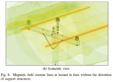
B. Magnetic field contours

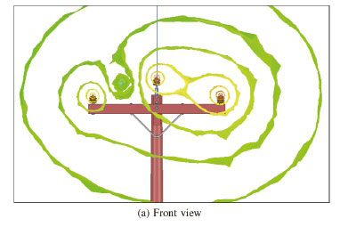
Figure 8 shows the simulation results of the instance which excludes the presence of materials with high magnetic field permeability. The concentric rings in Figure 8(a) show areas of equal magnetic field strength. By looking at the isometric view in Figure 8(b) it can be seen that these contour lines run parallel with the conductors, and are unchanged near the plane in which the cross-arm and most of the metal fixtures lie.

 

 

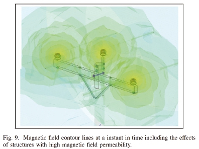
The second instance of the simulation was run, including the effects of the support structures. Figure 9 shows that these support structures do indeed distort the magnetic field. The magnetic field contour lines no longer run parallel with the conductors, and aggregate around the insulators. This is likely due to the galvanized steel bolts affixing the insulators to the wood beam, which are in close proximity to the conductors.

 

 

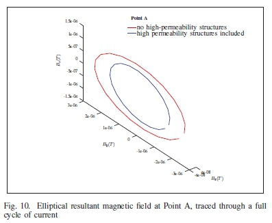
C. Resultant ellipses

The resultant magnetic field measured at Point A was plot as one full cycle of current energized the conductors, shown in Figure 10. The DC offset has been removed to aid in visual comparison. The data was processed using a least-squares curve fitting algorithm in order to extract the ellipse parameters, similar to the procedure in Section III-B. These ellipse parameters can be seen in Table I.

 

 

 

 

D. Results and discussion

By observing the plots in Figure 10 and the ellipse parameters in Table I, it can be seen that the presence of structures with high magnetic field permeability do indeed alter the resultant ellipse. This means that the proposed relationship in (14) must be modified to account for these effects, as the transformation from current to magnetic field is not based solely on geometry. This may not be possible since the construction of power line poles are not unique, and the location of materials with high magnetic field permeability is highly unpredictable.

The resultant magnetic field does, however, still retain its elliptical shape. This implies that the procedure used in Section III-B can still be used to characterize the geometric state of the power line, such that detecting a change in geometric state between poles is achievable. It is conceivable that a geometric fault can be detected, however, not necessarily the classification of the fault.

 

V. TEST HARDWARE

Figure 11 shows a proof of concept prototype device housing two 3-axis magnetic field sensors (MPU-92/65 by InvenSense); a wireless radio transceiver; a micro-controller; and a battery power supply. This device will be used to characterize the accuracy and repeatability of the 3-phase current measurement using two magnetic field sensors; test wireless communication of this information, and characterize the power requirements for the energy harvesting design. The processing of magnetic field measurements (reduction to ellipse parameters) will also be performed locally, as opposed to being streamed to a computer and then processed. A second prototype has since been designed and manufactured, featuring the previously mentioned magnetic field sensor MMC5883MA. The signal to noise ratio of sensor measurements is inversely proportional to the output data rate (ODR) of the sensor [15]. Lowering the ODR to achieve better signal quality may result in aliasing of the readings, and thus unpredictable results. A balance between these two parameters must be achieved. Various other circuitry has been included to measure other environmental metrics, a solar panel with MPPT charge controller, and an IP67 UV resistant enclosure. These modifications will allow the test hardware to provide more accurate magnetic field readings, and withstand long-term lab or field testing.

 

 

VI. Conclusion

This paper has reported on qualitative research into the behavior of distribution power line magnetic fields with respect to sensing with a MEMS device, as well as the concept design of a distribution line condition monitoring device. It is shown empirically that a change in geometry between poles (that support the same conductors) can be detected by characterizing the magnetic field, and sharing this information between poles.

It is shown through simulations that magnetic field distortions are present due to fixtures with high magnetic field permeability, but may not impede the unique characterization of the system geometry. In order to achieve true fault identification, machine learning methods may need to be implemented to determine the steady-state geometry of each pole, in order to mitigate these distortions and other geometric unknowns. A repeatable mathematical model may not be feasible given the non-uniform placement of metal structures near the conductors.

Future work includes testing of the prototype device at full geometric scale, and moving towards a technology demonstrator that can be field tested. The positioning of the sensors with relation to the conductors represents a crucial design decision as it will determine the accuracy of the system, the power source and therefore device lifetime, as well as the ease of installation. The protocol used to facilitate the transmission of data from the power line to the substation will greatly affect reliability and cost effectiveness of the device, given its contribution to energy budget, as well as the quality of service it renders to the utility provider. A successful low-cost implementation of this technologically feasible concept is realizable given the decrease in IoT technology prices.

 

Acknowledgment

This work was partially supported by the Eskom Tertiary Education Support Programme.

 

References

[1] Electricity Distribution System Baseline Report, U.S. Department of Energy, July 2016, pp. 11. [Online]. Available: https://energy.gov/epsa/downloads/electricity-distribution-system-baseline-report. [Accessed 11/2017].

[2] Eskom Integrated report 31 March 2017, pp. 114. [Online]. Available: http://www.eskom.co.za/IR2017/Documents/Eskom_integrated_report_2017.pdf. [Accessed 11/2017].

[3] R. A. Scott, "Comparison and Evaluation of South African Poletop Designs for 11kV and 22kV Rural Distribution Lines" MSc thesis, pp. 117, University of Cape Town, 1992.         [ Links ]

[4] G. S. Bhuyan, "Condition based serviceability and reliability assessment of wood pole structures," in Transmission & Distribution Construction, Operation & Live-Line Maintenance Proceedings. IEEE, 1998, pp. 333339.

[5] R. E. Harness and E. L. Walters, "Woodpeckers and utility pole damage," IEEE Industry Applications Magazine, vol. 11, no. 2, pp. 68-73, 2005.         [ Links ]

[6] K. Thejane, A. Beutel, M. Ntshani, H. Geldenhuys, A. Britten, W. Vosloo, T. Mvayo, R. Watson, R. Swinny, C. Evert et al., "Pole top fires: Review of work to date and a case for further research," in Power Engineering Society Conference and Exposition in Africa (PowerAfrica). IEEE, 2012.

[7] C. Ensing, "Sparks fly from electrical wires after vehicle crashes into pole" 24 June 2017. [Online]. Available: http://www.cbc.ca/news/canada/london/electrical-fire-starts-after-motor-vehicle-crash-with-explosions-1.4177037. [Accessed 11/2017].

[8] P. Rogers, M. Gafni, G. Avalos, "PG&E power lines linked to Wine Country fires", 10/10/2017. [Online]. Available: http://www.mercurynews.com/2017/10/10/pge-power-lines-linked-to-wine-country-fires/. [Accessed 11/2017].

[9] A. Ellam and G. Earp, "Understanding and defining overhead line investment requirements," in 41st Universities Power Engineering Conference., vol. 1. IEEE, 2006, pp. 237-241.

[10] A. A. Beutel, H. J. Geldenhuys, J. Van Coller and K. V Thejane, "Measurement and analysis of the electric and magnetic field on a 22 kV woodpole distribution line," in 19th International Symposium on High Voltage Engineering, CIGRE, 2015.

[11] Schweitzer Engineering Laboratories, "WSO-11 wireless sensor for overhead lines," WSO-11 datasheet, August 2015.

[12] X. Sun, Q. Huang, Y. Hou, L. Jiang, and P. W. Pong, "Noncontact operation-state monitoring technology based on magnetic-field sensing for overhead high-voltage transmission lines," IEEE Transactions on Power Delivery, vol. 28, no. 4, pp. 2145-2153, 2013.         [ Links ]

[13] A. H. Khawaja, Q. Huang, J. Li, and Z. Zhang, "Estimation of current and sag in overhead power transmission lines with optimized magnetic field sensor array placement," IEEE Transactions on Magnetics, vol. 53, no. 5, pp. 1-10, 2017.         [ Links ]

[14] Apparatus and method for remote current sensing, by N. P. Tobin. (1999, Nov. 12). US6727682B1. Accessed on: June. 2, 2017. [Online]. Available: https://patents.google.com/patent/US6727682B1/en

[15] MEMSIC, "High Performance, Low Cost 3-axis Magnetic Sensor," MMC5883MA datasheet Rev. C, April 2017.

[16] MeshLogic. (2018). Fitting a Circle to Cluster of 3D Points. [online] Available: https://meshlogic.github.io/posts/jupyter/curve-fitting/fitting-a-circle-to-cluster-of-3d-points/ [Accessed 15 Feb. 2018].

[17] Mathworks.com. (2018). fitellipse File Exchange - MATLAB Central. [online] Available: https://www.mathworks.com/matlabcentral/fileexchange/3215-fit-ellipse [Accessed 6 Jul. 2017].

[18] A. Y. Wang and C. G. Sodini, "On the energy efficiency of wireless transceivers," in Communications, ÏCC06. I, vol. 8. IEEE, 2006, pp. 3783-3788.

[19] USDA, "Specifications and Drawings for 24.9/14.4 kV Line Construction" in RUS Bulletin, 1728F-803(D-803), December 1998, pp. 195. [online] Available: https://www.rd.usda.gov/files/UEP_Bulletin_1728F-803.pdf [Accessed 16 April 2018]

 

 

 

Jason Hardy received the B.Sc degree in Mechatronics from the University of Cape Town in 2015, where he is currently a M.Sc candidate and teaching assistant.
He has worked in the power generation sector on various mines in Africa. He was one of the founders of a student initiative to install coffee vending machines at the University of Cape Town. This necessitated the use of remote monitoring and cashless payment systems, which he developed and implemented.

 

 

Edward Boje currently a Professor and Head of Electrical Engineering at the University of Cape Town. Prof. was formerly Deputy Dean of Engineering at the University of KwaZulu-Natal.
He has undertaken research and consulting work in the field of control systems, quantitative feedback design, system identification, state estimation and power line robotics. This work has led to publication of over 80 papers in journals and conferences, two book chapters, three SA patents, and a US patent. He has industrial experience in the biotechnology, process instrumentation and control, paper and pulp, defense, mining and electrical power (generation and transmission) industries. He has presented seminars and short courses in industry and at universities both nationally and internationally. He was the international programme committee co-chair of the 2014 International Federation of Automatic Control (IFAC) World Congress and was a member of IFACs Technical Board (2014-2017).
Prof. Boje is a registered professional engineer in South Africa, a Fellow of the SA Academy of Engineering and a Member of the IEEE.