


Serviços Personalizados
Artigo
 Inglês (pdf)
 Artigo em XML
 Referências do artigo
Indicadores

Links relacionados
-
 Citado por Google
 -
 Similares em Google
Compartilhar

 Permalink
SAIEE Africa Research Journal
versão On-line ISSN 1991-1696
versão impressa ISSN 0038-2221
SAIEE ARJ vol.109 no.4 Observatory, Johannesburg Dez. 2018
ARTICLES
Time series analysis of impulsive noise in power line communication (PLC) networks
S. O. AwinoI; T. J. O. AfulloII; M. MosalaosiIII; P. O. AkuonIV
IDiscipline of Electrical, Electronic & Computer Engineering, School of Engineering, University of KwaZulu Natal, Durban, 4041, South Africa E-mail: 215080505@stu.ukzn.ac.za
IIDiscipline of Electrical, Electronic & Computer Engineering, School of Engineering, University of KwaZulu Natal, Durban, 4041, South Africa E-mail: Afullot@ukzn.ac.za
IIIDiscipline of Electrical, Electronic & Computer Engineering, School of Engineering, University of KwaZulu Natal, Durban, 4041, South Africa E-mail: mezmerizemod@gmail.com
IVDepartment of Electrical & Information Engineering, University of Nairobi, P.O. Box 30197 - 00100, Nairobi, Kenya E-mail:akuonp@yahoo.com, akuon@uonbi.ac.ke
ABSTRACT
This paper proposes and discusses Autoregressive Moving Average (ARMA), Autoregressive Integrated Moving Average (ARIMA) and Seasonal Autoregressive Integrated Moving Average (SARIMA) time series models for broadband power line communication (PLC) networks with impulsive noise enviroment in the frequency range of 1 - 30 MHz. In time series modelling and analysis, time series models are fitted to the acquired time series describing the system for purposes which include simulation, forecasting, trend assessment, and a better understanding of the dynamics of the impulsive noise in PLC systems. Also, because the acquired impulsive noise measurement data are observations made over time, time series models constitute important statistical tools for use in solving the problem of impulsive noise modelling and forecasting in PLC. In fact, the time series and other statistical methods presented in numerous available literature draw upon research developments from two areas of environmetrics called stochastic hydrology and statistical water quality modelling as well as research contributions from the field of statistics. In time series modelling and analysis, we determine the most appropriate stochastic or time series model to fit our acquired data set at the confirmatory data analysis stage. No matter what type of stochastic model is to be fitted to the data set, we follow the identification, estimation, and diagnostic check stages of model construction. In addition, we explore the resulting autocorrelation functions in estimating the parameters of the selected time series models. Finally, SARIMA model is found suitable for computer-based PLC systems simulations and forecasting based on the diagnostic checks.
Keywords: PLC, power line network, impulsive noise, ARMA models, ARIMA models, SARIMA models, autocorrelation function
1. INTRODUCTION
Power line communication (PLC) is a technology that involves the transmission of communication signals through the existing high voltage low frequency power distribution grid. It is a technology that evolved soon after the widespread establishment of the electrical power supply distribution systems [1]. Because of the high costs incurred in installation of new infrastructure for new communication systems, PLC offers an alternative solution for the realization of the access networks using the existing power supply grids for communications. Thus, for the realization of the PLC networks, there is no need for the laying of new communications infrastructure. Therefore, application of PLC in low-voltage supply networks seems to be a cost effective solution for the low-voltage in-door communication networks [2].
However, the power line network is characterized as unstable channel because of its ever varying impedance, frequency dependent attenuation, multipath fading and propagation due to the numerous branching as well as impulsive noise caused by the 'ON' and 'OFF' switching of electrical appliances connected to the power line network. Contrary to other available communication channels, the noise in power line channels cannot be described by an additive white Gaussian noise (AWGN) model [3]. Thus, a thorough analysis and understanding of the power line network as a channel of communication is an inevitable prerequisite for appropriate modelling, a task that was carried out by the author in [4, 5] when investigating the channel properties of low-voltage power line networks. Preliminary measurement results from Vines et al [7], Zimmerman and Dostert [3], and Meng et al [6] among other researchers, have showed that the impulsive noise levels depended dramatically on which electrical loads were currently in use. This fuelled studies to determining the major sources of noise in the power line networks and their associated noise characteristics, studies which are well detailed in [3,6,7]. Besides such studies, recent surveys in PLC noise models have also grouped the noise models into models with memory and memoryless models [8,9]. Because of the bursty nature of the impulsive noise in the power line network, it is also referred to as bursty impulsive noise [10, 11]. In the work of Asiyo and Afullo [10, 12], the bursty nature of PLC noise and its frequency of occurrence were investigated and found to posses long range dependence and multiscaling behaviour which is a characteristic of a system with memory.
But even with all the aforementioned unresolved challenges that form the most crucial properties of power line networks that degrade the performance of high-speed communications, PLC is developing as one of the strong competitors in the broadband communication market for in-door communication in the frequency range from 1 -30 MHz [6]. Of recent, much attention has been focused on addressing the impulsive noise in PLC. In the work of Gianaroli et al [13], an algorithm is developed to make the measured noise series stationary to allow for application of a stationary Autoregressive moving average (ARMA) model, while in Mosalaosi's work [14], PLC noise is described as a generalized autoregressive conditional heteroskedastic (GARCH) process based on the idea that PLC noise exhibits volatility clustering. However, both ARMA and GARCH models, fail to account for the seasonal behaviour of PLC impulsive noise, a key property that cannot be assumed and diminished.
Thus, in a concerted effort to extend the knowledge about impulsive noise modelling in PLC, our approach is by a measurement based analysis of the fundamental properties in the frequency range of 1 - 30 MHz using ARMA, ARDVIA and SARIMA time series models. The use of these statistical techniques enhance the scientific method which in turn means that the pressing problem of PLC impulsive noise modelling can be more efficiently and expeditiously solved. When carrying out a scientific data analysis study using PLC impulsive noise time series, we employ both exploratory data analysis and confirmatory data analysis tools. The purpose of exploratory data analysis is to use simple graphical methods (autocorrelation functions) to uncover the basic statistical characteristics of the data which can then be modelled formally at the confirmatory data analysis stage utilizing time series models. The motivation to applying these models in PLC noise modelling in this study are: 1. How applicable is integrated (also known as differencing) time series models to modelling PLC network noise, 2. To what extent can we integrate PLC noise data to achieve some level of stationarity without complex algorithms and 3. To develop a suitable time series model for simulation and forecasting of impulsive noise in PLC systems that will enable for an efficient and effective bit and power allocation algorithm with impulsive noise environment.
The rest of the paper is organized as follows: In Section 2., we present the measurement set-up and differencing as used in preprocessing the measured PLC impulsive noise data, while a brief theoretical frame work on time series models for PLC impulsive noise is discussed in Section 3.. In Section 4., we outline how time series models are systematically identified and selected to fit the measured data set. Results and diagnostic checks for the fitted models are then presented in Section 5. to chose a penurious model. Finally, the paper ends with concluding remarks in Section 6.
2. MEASUREMENT SET-UP AND DATA PROCESSING
The characterization of impulsive PLC noise requires an extensive experimental activity that can be carried out either at the port where the receiver coupler is connected or at the ports where the main sources of noise are connected. The former approach provides information about the overall noise that impairs communication in the power line channel. While the latter approach allows for the characterization of the main sources of noise by evaluating the level of disturbance that they individually inject in a certain point of the power line network [15]. In this work, we apply the former approach at selected locations for our study.
2.1 Measurement Set-up
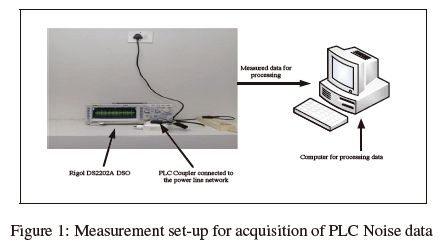
Sample measurement data were collected using a higher resolution Rigol DS2202A digital storage oscilloscope (DSO). The DSO is capable of recording 14 million data samples and was set to sample at a rate of 50 Mega-samples per second resulting in a window length of 0.28 seconds (14 mains cycles). Measurement data was similarly acquired from an electronic laboratory, a postgraduate office and from an isolated five roomed apartment using the DSO. The DSO was connected to the power socket via a coupling circuit as shown in the set-up of Figure 1. The coupling circuit ensured isolation and safety of the DSO from the power line network in addition to ensuring our operating frequencies to be within 1 - 30 MHz.
2.2 Description of Power Line Network Loading at Locations Under Study
Herein, we provide a detailed description of the electric devices connected to the various power line networks at each location.
-
Electronic laboratory: In this location, power line network loading is composed of fluorescent lights, air conditioners and numerous workstations serving 120 students per session. Each workstation is composed of a function generator, digital multimeter, cathode ray oscilloscope, electronic trainer board and triple output DC power supply. The electrical wiring is such that three workstations are connected to a single circuit breaker at the distribution board forming a single network. We acquired measurement results at the peak usage of this laboratory which started from 2:00 pm to 5:00 pm when students were undertaking their practicals. At this time, all the aforementioned equipments at the various workstations, fluorescent lights and the air conditioners are turned 'ON' and run throughout the session.
-
Postgraduate office: The electric devices connected to this power line network included: fluorescent lights, desktop and laptop computers, two air conditioner units, electric kettle and a shared Konica Minolta C364 series heavy duty printer serving 100 postgraduate students within the discipline. This office is fully occupied from 8:00 am to 5:00 pm before the occupants leave for their residences. Measurement data were acquired at multiple times during the day.
-
Residential apartment: This is an isolated five roomed apartment and contains: light dimmers, fluorescent lights, cathode ray tube (CRT) television set, washing machine, two fridges, iron box, a vacuum cleaner, thermostat electric kettle, water heater, electric cooker, juice blenders, microwave oven and security lights. Measurements were done at a time when all residents of the house were at home. That is in the evening from 6:00 pm to 10:00 pm. At this time, the use of electric appliances in the house is at its peak, washing machine turned 'ON', fridge doors opened at random, house lighting and security lights turned 'ON', the CRT television set and laptops being switched and left 'ON', water heating using thermostat electric kettle among other random events.
In the earlier research work of Meng et al [6] and Vines et al [7] among others addressing impulsive noise sources in PLC systems, lightning, thermostats, switched mode power supplies and other switching phenomena (as well as capacitor banks being switched in and out for power-factor correction) were found to cause impulsive noise. Recently, fluorescent lamps have been confirmed to inject impulsive noise levels that compete with the electromagnetic interference levels. These have a detrimental effect on PLC systems since they contain power electronic converters and electronic ballasts that act as noise sources in the power line channel in the frequency range of 150 KHz - 30 MHz (See Emleh, de Beer et al [16,17]). Additionally, in the work of Antoniali et al [15] and Tlich et al [18], power switches, power supplies, various domestic appliances, rectifiers within DC power supplies and devices such as thyristor/triac-based light dimmers have been confirmed to inject impulsive noise in the power line network. In the measurement environments under study, there is a strong presence of similar appliances and devices (See for example in Asiyo and Afullo in [10,12], Modisa and Afullo in [14], Nyete et al in [27] and Awino and Afullo in [4]).
2.3 Acquired Measurements results
A sample of the acquired measurement results within a window length of 0.28 seconds are as shown in Figures 2, 3 and 4. In order to analyze the acquired data, a digital bandpass filter was designed and implemented in Matlab to filter out unwanted noise components outside the desired frequency range of 1 - 30 MHz.


From the measured noise data, it can be seen that each of the different environments generate unique noise samples due to different noise sources. Even though there appears to be no obvious upward or downward trend in the measurement window presented in Figures 2, 3 and 4, the seasonal series are stationary within each season and the seasonality is clearly visible as a sinusoidal pattern wrapped around the trend of the mains cycle envelope.
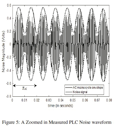
This occurs due to the periodic nature of impulsive noise synchronous to the mains frequency, which is mainly caused by switching actions of silicon controlled rectifiers (SCRs) and rectifier diodes found in the power supply of many electrical appliances as confirmed by Vines et al [7], Meng et al [6], Zimmerman and Dostert [3] and Gotz et al [19]. An SCR switches when the power voltage crosses a certain threshold. Because this voltage is cyclic, the SCR switches at 50 Hz or multiple of 50 Hz and thereby causing noise at 50 Hz and multiples thereof synchronous with, and drift with, the 50 Hz power frequency [7]. This is illustrated by the waveform in Figure 5. This figure shows the periodic impulsive noise over 0.08 seconds which corresponds to four mains power supply voltage cycles. This waveform in Fig. 5, shows that noise characteristics change synchronously with a period TAC/2, where TAC refers to the cycle duration of the mains power supply voltage [20].
2.4 Differencing Analogy in Processing PLC Noise Data
PLC noise is a nonstationary time series process whose statistical properties change over very short time intervals. When considering shorter time series, its often reasonable to assume that a stationary model can adequately model the data. When dealing with continuous data, a differencing parameter corresponding to the integrated part of the model, is employed to remove homogeneous nonstationarity [21], a technique which is analogous to differentiation. Consider for example, a continuous function of time which is given by [21]

where c is a constant that reflects a local level for t ≥ T. The derivative of  will be zero for t > T and the local level due to the constant c drops due to differentiation. To consider the analogous effect of the differencing operator of the second derivative for a continuous function, let a continuous function of t be given as [21]

with c and b being constants. The term, (c + bt), forms a linear deterministic trend of the process yt. The value of the first derivative is  , while
  .Hence, the intercept c is removed from the first derivative, while the linear function is completely eliminated by the second derivative. While differencing the data, it is advisable to select the lowest order of differencing for the data to preserve as much content of the data as possible. In this work, we consider non-differencing, nonseasonal differencing as well as seasonal differencing and compare their performances.
3. THEORETICAL FRAME WORK ON TIME SERIES MODELS FOR PLC IMPULSIVE NOISE
Time series analysis has been widely employed in many water resources projects in hydrology, stock exchange analysis in econometrics and statistical works as evidenced in [22-24]. However, this has not been the case in PLC noise modelling problem with the first attempts presented in [13] to model the impulsive nature of PLC noise using stationary Box-Jenkins model. The Box-Jenkins approach is based on the use of stationary ARMA models to predict and forecast time series. However, impulsive PLC noise data exhibit characteristics that are more seasonal and nonstationary and as a consequence will require removal of nonseasonal and seasonal nonstationarities using nonseasonal and seasonal differencing operators, respectively before fitting a stationary ARMA, ARIMA and SARIMA models to the series.
3.1 ARMA and ARIMA Models For PLC Impulsive Noise
A time series yt is ARMA (p, q) if it is stationary and

with  . If yt has none zero mean set
  and write the model as [25],

This can be written in concise form as [21,25],
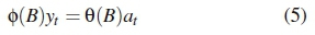
where Вis the backward-shift operator, ф(В) and 0(B) are the autoregressive, AR(p) and moving average, MA(q) operators respectively and at is a white noise series characterized by independent identically distributed (i.i.d) random variates with mean zero and variance  . By including differencing, ytcan be said to be ARIMA (p, d, q) if [21,25]
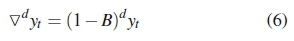
where  is the differencing operator defined by
  yt = yt - yt-1and d is an integer assumed to be a positive when the series must be differenced to remove non-stationarity.
3.2 SARIMA models For PLC Impulsive Noise
Due to a strong and well established seasonal pattern in our series, we employ seasonal differencing differencing for the proposed SARIMA model. This is done so that the seasonality pattern does not 'die out' in the long term forecast. SARIMA model is defined by the following (P, D, Q), where the parameters P, D and Q are the order of seasonal autoregressive average (SAR), order of seasonal differencing and order of seasonal moving average (SMA) respectively. Thus the complete model is called an 'ARIMA (p,d,q) x (P,D, Q)' model [21,25]. To make the series stationary, we combine seasonal and nonseasonal differencing as,
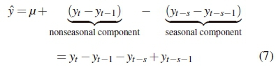
where s is the seasonal period of 40 data points in this study. Note that D should never be greater than one and d + D ≤2. And if d + D = 2, then the constant term \i is suppressed as given by (7) which is a difference equation form. Thus, by rewriting (7) in a general form, SARIMA model will be given by [25]

where  and
and  define the SAR parameter of order P, SMA parameter of order Q, seasonal backshift operator and seasonal difference component respectively.
The other parameters bear their usual meanings. Also, because of the differencing process, the differenced series wt, is d - sD shorter than the original series with d being the orderof non-seasonal differencing, D is the orderofthe seasonal differencing while s refers to the periodic seasonal behaviour of the original series. The length of the wtseries will be defined by
with N being the length of original series.
4. MODELS IDENTIFICATION AND SELECTION
A key modelling principle for any process is to have as few parameters as possible for a given model [21]. In time series analysis for example, if a sample autocorrelation function (ACF) for a given data set has a value that is significantly different from zero only at a given specific lag k, then it is appropriate to fit a MA model whose order is defined by the lag to the data. Similarly, when the partial autocorrelation function (PACF) for the data cuts off at a given lag k, then it is most appropriate to fit an AR model whose order is defined by the value of the lag at that point. In a situation where both sample ACF and PACF cuts off for certain time series, then it is advantageous to have a model that contains both the AR and MA parameters. This ensures, the fitted model has few parameters as possible. Because, we are dealing with a nonstationary time series data, we apply differencing to the data to make it stationary. To determine the order (p, q) and (P, Q), and estimate the model parameters, ф к and Өk, and Ф к and өk, respectively, we resort to the ACF and PACF as the main tools in the process. On the other hand, parameters d and D are defined by the order of nonseasonal and seasonal differencing respectively applied to the data at preprocessing stage. In this section we employ autocorrelation functions to identify possible models for the measured data and thereafter, perform a model selection process based on Akaike's information criteria (AIC).
4.1 Structure of Autocorrelations For Model identification
Model identification involves the selection and choice of the order p, d, q and P, D, Q of the model. Based on the recommendation of Box-Jenkins models, the parameters p and P, q and Q are chosen through a graphical approach by looking at the ACF and PACF values versus the lag of the non-differenced and differenced series. Given a sample from the observed data y0,y1,y2,...,yN, we can define the sample AC F to be a sequence of values [21,25]

is the autocovariance at lag k and y0 is the sample variance. Thus, to identify the type of time series model to fit a given time series data of length N, we check for significant values from the ACF plot. On the other hand, a sample PACF, р к at lag кrefers to the correlation between two sets of residuals obtained from regressing the elements ytand yt-k on the set of intermediate values y1,y2,y3,...,yt-k+1. It is actually a measure of the dependence between ytand yt-k after removing the intermediate values.
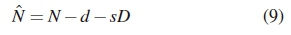
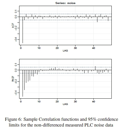
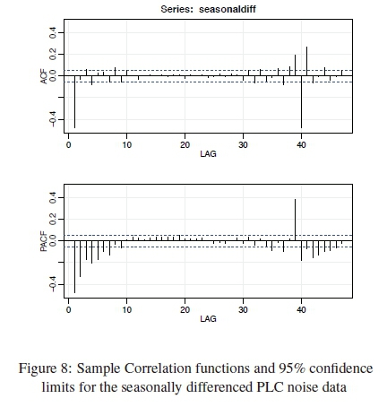
In order to identify the number of AR, MA, SAR and SMA terms required in the model of the non-differenced and differenced series, the sample ACF and its associated PACF are interpreted simultaneously keeping in mind the main identification rules that the ACF cuts-off for pure MA processes, while the PACF truncates for AR models. For mixed processes, both functions attenuate. The autocorrelation functions are as shown in Figures 6, 7 and 8 for non-differenced and differenced PLC noise time series data respectively.
Interestingly, from Figure 6, ARMA models can be applied to model the PLC noise data since the autocorrelation functions truncates at a definite lag as the lags increases to infinity. This is also observed from Figure 7 for ARIMA models even though with a few noticeable significant spikes as the lags increases. From Figure 8, we observe a negative significant spike in the ACF at lag 1 and also at lag 40, whereas the PACF shows a gradual decay pattern in the neighbourhood of both lags. These denotes an MA and SMA signatures respectively in time series analysis. SARIMA models depend on seasonal lags and differences to fit the seasonal patterns. When the process is a pure MA(0, d, q) x (0, P, Q), model, the sample ACF cuts-off and is not significantly different from zero after lag q + sQ. Also, notice that the coefficient of lag 41 error is approximately a product of MA (1) and SMA (1) coefficients. There is a slight surprise at lag 39 since we observe significant spikes on the autocorrelation. This can be attributed to the covariance between the terms ytand y39 not being equal to zero.
4.2 Akaike's information criteria (AIC) for model selection
After several possible models were fitted, an optimal model were then selected by using the Akaike's information criteria (AIC) (11) [26] for each as reported in Table 1.


where N is the number of data points,  is the number of parameters in a given model and SS is the regression sum of squares defined by

From the various AIC values reported in Table 1, non-differenced ARMA models seems to have the lowest AIC values as compared to the other integrated models.
After the optimal lag lengths selection using the AIC values, three candidate models are obtained. We move ahead to model the series as an ARMA (0,0,1), ARIMA (1,1,1) and SARIMA (0,0,1) x (0,1,1) process. The result of the estimated parameters of ARMA (0,0,1), ARIMA (1,1,1) and SARIMA (0,0,1) x (0,1,1) models are as shown in Table 2. This calls for fitting of the models and the estimated parameters are fitted. Thus,
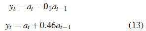

for ARMA (0,0,1) model,

for ARIMA (0,0,1) model. And lastly

for SARIMA (0,0,1) x (0,1,1) model (since d + D < 2). Equations (13), (14) and (15) are the closed-form solutions from the analysis. In the work of Gianaroli [13], they employed higher order ARMA models. This is due to the fact that in time series models, the autocorrelation functions fail to converge because significant 'spike' terms do not approach zero 'fast enough' as expected as the lags tend to infinity. We encountered such a scenario in the course of our analysis as well. However, based on the definitions obtained from the correlation functions and AIC values reported in Table 1, we formalized the solutions mathematically by considering only models with the lowest AIC values and had the most significant 'spike' terms at the early lags. Having fitted the models to the times series, we check the adequacy of the models through diagnostic checks.
5. RESULTS AND DIAGNOSTIC CHECKS
In this section, the measured impulsive PLC noise series is analyzed using the ARMA, ARIMA and SARIMA time series models of (13), (14) and (15) respectively. Model validation and diagnostic checks which are concerned with checking the residuals of the models are done to see if they contain any systematic pattern which still could be removed to improve the chosen models. The results for the models are as presented in Figures 9, 10 and 11 for ARMA, ARIMA and SARIMA models respectively. Only validation results of models with the lowest AIC values are presented for each class.


For ARMA models, the effect of having the AR (1) and MA (1) components is evident from the AIC values. For the AR (1) model, it is simply a linear regression model that predicts the current value from immediate prior value in time. Actually, the current value is assumed to be a linear combination of previous values. The MA (1) model assumes the current values are linear combinations of the previous error terms and consequently has the lowest AIC value. Thus, when the two components are combined into ARMA (1,0, 1) model, their effect is equivalent to having two MA (2) parameters within the same model.
For ARIMA models, the effect of nonseasonal differencing on the series data is random walks without drift as evidenced by the highest AIC value (i.e ARIMA (0, 1, 0)). By introducing an MA (1) component, we are simply correcting the autocorrelated errors in the random walks through exponential smoothing. On the other hand, an AR (1) component also corrects the autocorrelated errors in the random walks by regressing the first difference of the predicted value on its own lagged values by one period. Having both AR (1) and MA (1) components, ARIMA (1, 1, 1) results to a reduced AIC value. This is because the model is estimating the predicted value outside the known range (local trend) at the end of the series while exponentially smoothing it at longer forecast levels to introduce conservation.
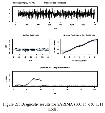
Lastly, for SARIMA models, exponential smoothing to level, trend and seasonality is applied at the same time. Firstly, the difference between each season's value and an exponentially weighted previous average for that season is determined by applying exponential smoothing observed in the previous season in which the SMA (1) coefficient determines the length of the smoothing. An exponential smoothing is then applied to these differences to enable prediction of the deviation from the previous average that will be observed next season. The SMA (1) coefficient suggests that a little smoothing is applied to estimate the current deviation from the previous average. This means that next season's predicted deviation from previous average is close to the deviation from previous average observed over the last few seasons.
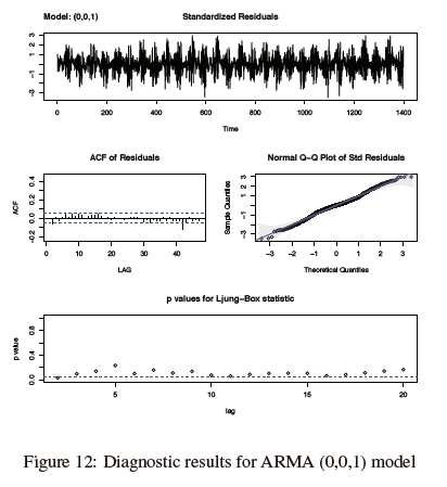
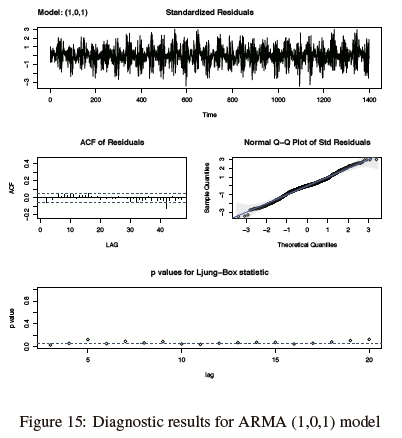
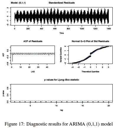
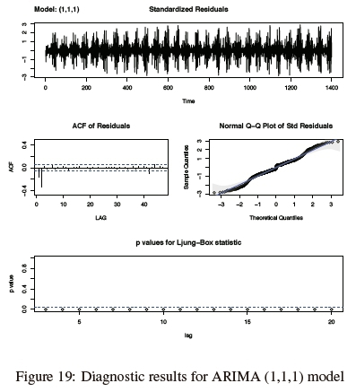
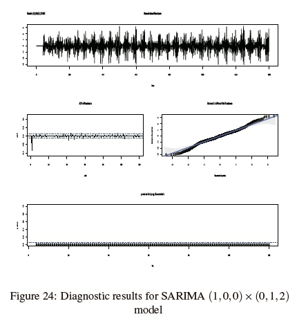
Even though all the models look to capture the measured data very well based on the validation results presented in Figures 9, 10 and 11, we performed diagnostic checks on their residuals and are as reported in Figures 12,13,14,15, 16, 17, 18, 19, 20, 21, 22, 23, 24.


5.1 ACF of Standardized Residuals
To check the adequacy of the models, the process of diagnostics were conveniently carried out based on their residuals. For an adequate model, the residuals should behave as an i.i.d sequence with mean zero and variance one and were based on the recommended autocorrelations of the residuals. From the standardized residual plots, all the model residuals behave as an i.i.d sequence with mean zero and variance one except for ARIMA models.
From the ACF plots, very significant spikes can be observed at lower lags for ARMA (1, 0, 0), all ARIMA, SARIMA (0,0,1) x (0,1,1) and SARIMA (1,0,0) x (0,1,2) models. This is a clear indicator of unwanted correlation in model residual, hence these models are inadequate. The remaining models have fairly random residuals with a few incidence of significant correlations which can be ignored, hence adequate.
5.2 Normal Quantile-Quantile plots (QQ plots)
Also, investigation of marginal normality for these models were accomplished by looking at their normal quantile-quantile plots (QQ plots) which helped identify departures from normality. Interestingly, the all the residuals are normally distributed as can be observed from the QQ plots except for the ARIMA models. This is a pointer on the inadequacy of nonseasonal differencing when used own its own on seasonal time series data.
5.3 Ljung-Box Statistic Analysis of autocorrelation values
The Ljung-Box statistics, also called modified Box-Pierce statistic, is a function of the accumulated sample autocorrelations ri, up to any specified time lag k [25]. Thus, as a function of k, it is given as [21,22,25]
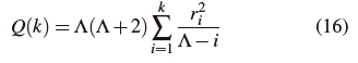
where Л is the number of usable data points given by N and NN for non-differenced and differenced series respectively. In order to determine the p-value, we calculate the probability past Q(k) in the relevant distribution. A small p-value (for instance, p-value< 0.05) indicates the possibility of non-significant autocorrelation within the first k lags. Thus, for an adequate model, the desired p-values should be well above 0.05 as can be observed for ARMA models. Also, SARIMA (0,0,1) x (0,1,1) and SARIMA (1,0,1) x (0,1,1) models have greater p-values from lag 1 to lag 42, which is a fairly large range and therefore accepted.
5.4 Root Mean Square Errors (RMSE)
After carrying out model selection, validation and diagnostics checks, performance analysis for selected models based on their residuals were undertaken. Residuals are simply the difference between the predicted values and actual measured values, denoted by y - yt, where y is the predicted value and ytis the actual measured value. The residual values assumes both positive and negative values depending on whether either the predicted value over estimated or under estimated the actual measured value. By squaring the residuals, averaging the squares and taking the square root, we obtain the Root mean square errors (RMSE). Mathematically, the RMSE is defined as

where N is the number of samples. The RMSE is employed to measure the accuracy of forecast of ARMA, ARIMA and SARIMA models and thereafter a penurious model would be chosen. Table 3 shows the RMSE results.
From the results in Table 3, the RMSE value of ARIMA (1,1,1) model is the highest. The RMSE values ARMA (0, 0, 1) and SARIMA (0,0,1) x (0,1,1) models are quite close. We can therefore conclude that SARIMA (0,0,1) x (0,1,1) model is a much better model than the ARIMA (1,1,1) in modelling the impulsive PLC noise, even though ARMA (0,0,1) model still performs better.
6. CONCLUSIONS
In this paper, we have modelled and conducted a forecast of the impulsive noise experienced in the power line network using ARMA, ARIMA and SARIMA time series models. SARIMA models have been motivated by the existence of seasonality in the measured series. From the autocorrelation functions of the measured PLC noise characteristics, suitable ARMA, ARIMA and SARIMA models were identified, fitted and optimal models selected through the AIC. Even though all the models seemed to have fitted the data very well, ARIMA models scored poorly based on the diagnostic checks. In addition, forecasts obtained using the SARIMA models seemed much closer to the measured values than forecasts obtained using ARMA and ARIMA models. This was confirmed by forecast evaluation using RMSE and showed that SARIMA models are much better than ARMA and ARIMA models. Based on our data, we can therefore conclude that PLC noise modelling is better modelled by SARIMA models, and also that seasonal differencing is very effective as compared to nonseasonal differencing. Now that we can correctly and accurately forecast the impulsive noise component in the power line network, further work will be to study and implement an effective and efficient bit and power allocation algorithm with considerations on the uniformity of power for PLC systems with impulsive noise environment.
ACKNOWLEDGEMENT
This work was partially supported by the School of Engineering, University of KwaZulu Natal.
REFERENCES
[1] J. Anatory andN. Theethayi: Broadband power-line communication systems: Theory and applications, WIT Press, 2010.
[2] H. Hrasnica, A. Haidine and R. Lehnertand: Broadband powerline communications networks: Network design, John Wiley& Sons Ltd, UK, 2004.
[3] M. Zimmermann and K. Dostert: "Analysis and modelling of impulsive noise in broadband power line communications", IEEE Trans. On Electromagn. Comp., Vol. 44 No. 1, pp. 250-258, February 2002. [ Links ]
[4] S.O. Awino and T.J.O. Afullo: "Measurements and multipart) characterization of power line communication channel", Proceedings: 24th South African Universities Power Engineering Conference (SAUPEC), Vaal University of technology, Gauteng, South Africa, pp. 353-360, January 2016.
[5] S.O. Awino and T.J.O. Afullo: "Power line communication channel modelling using parallel resonant circuits approach", Proceedings: South Africa Telecommunication Networks and Applications Conference (SATNAC), Western Cape, South Africa, pp. 353-357, September 2015.
[6] H. Meng, Y.L. Guan and S. Chen: "Modeling and analysis of noise effects on broadband power line communications", IEEE Trans. On Power Delivery, Vol. 20 No. 2, pp. 630-637, April 2005. [ Links ]
[7] R.M. Vines, H.J. Trissell, L.J. Gale and J.B. O'Neal: "Noise on residential power distribution circuits", IEEE Trans. On Electromagn. Comp., Vol. EMC-26, No. 4, pp. 161-168, November 1984. [ Links ]
[8] S.P. Herath, N.H. Tran, and T. Le-Ngoc: "On optimal input distribution and capacity limit of Bernoulli-Gaussian impulsive noise channels", Proceedings: IEEE Int. Conference On Commun. (ICC), Ottawa, Canada, pp. 3429-3433, June 2012.
[9] T. Shongwe, A.J. Han Vinck and H.C. Ferreira: "A study on impulse noise and its models",SAIEE Africa Research Journal, Vol. 106 No. 3, pp. 119-131, September 2015. [ Links ]
[10] M.O. Asiyo and T.J.O. Afullo: "Analysis of bursty impulsive noise in low-voltage indoor power line communication channels: Local scaling be-haviour",SAIEE Africa Research Journal, Vol. 108 No. 3, pp. 98-107, September 2017. [ Links ]
[11] G. Ndo, F. Labeau, and M. Kassouf: "A Markov-Middleton model for bursty impulsive noise: Modeling and receiver design", IEEE Trans. On Power Delivery, Vol. 28, No. 4, pp. 2317-2325, October 2013. [ Links ]
[12] M.O. Asiyo and T.J.O. Afullo: "Prediction of long-range dependence in cyclostationary noise in low-voltage PLC networks", Proceedings: Progress of Electromagn. Research Symposium , Shanghai, China, pp. 4954-4958, August 2016.
[13] F. Gianaroli, F. Pancaldi, E. Sironi, M. Vigilante, G.M. Vitetta and A. Barbieri: "Statistical modeling of periodic impulsive noise in indoor power-line channels", IEEE Trans. On Power Delivery, Vol. 27, No. 3, pp. 1276-1283, July 2012. [ Links ]
[14] M. Mosalaosi and T.J.O. Afullo: "Prediction of asynchronous impulsive noise volatility for indoor power line communication systems using GARCH models", Proceedings: Progress of Electromagn. Research Symposium, Shanghai, China, pp. 4876-4880, August 2016.
[15] M. Antoniali, F. Versolatto and A.M. Tonello: "An experimental characterization of the PLC noise at the Source", IEEE Trans. On Power Delivery, Vol. 20, No. 2, pp. 630-637, April 2005. [ Links ]
[16] A. Emleh, A.S. de Beer , H.C. Ferreira and A.J. Han Vinck, "The influence of fluorescent lamps with electronic ballast on the low voltage PLC network," in Proceedings: IEEE 8th International Power Engineering and Optimization Conference (PEOCO2014), The Jewel of Kedah, Malaysia, pp.276-280 , March 2014.
[17] A. Emleh, A.S. de Beer , H.C. Ferreira and A.J. Han Vinck, "The impact of the CFL lamps on the power-line communications channel," in Proceedings: IEEE Int. Symposium on Power Line Communications and Its Applications (ISPLC), Johannesburg, South Africa, pp.225-229 , March 2013.
[18] M. Tlich, H. Chaouche, A. Zeddam and F. Gauthier: "Impulsive noise characterization at source", Proceedings: 2008 1st IFIP Wireless Days (WD), Dubai, United Arab Emirates, pp. 1-6, November 2008.
[19] M. Gotz, M. Rapp and K. Dostert: "Power line channel characteristics and their effect on Communication system design", IEEE Commun. Magazine, Vol. 42, No. 4, pp. 78-86, April 2004. [ Links ]
[20] Y. Hirayama, H. Okada, T. Yamazato and M. Katayama: "Noise analysis on wide-band PLC with high sampling rate and long observation time", Proceedings: IEEE Int. Symposium on Power Line Communications and Its Applications (ISPLC), Kyoto, Japan, pp. 142-147, March 2003.
[21] K.W. Hipel and A.I. McLeod: Time series modelling of water resources and environmental systems, Elsevier Science, Netherlands, 1994.
[22] V. Reisen: "Estimation of the fractional difference parameter in the ARIMA (p, d, q) model using the Smoothed Periodogram", Journal of Time Series Analysis, Vol. 15 No. 3, pp. 335-350, March 1994. [ Links ]
[23] J. Giweke and S.P. Hudak: "The estimation and application of long memory time series models", Journal of Time Series Analysis, Vol. 4 No. 4, pp. 221-238, April 1983. [ Links ]
[24] G. Saz: "The efficacy of SARIMA models for forecasting inflation rates in developing countries: The case for Turkey", Int. Research Journal of Finance and Economics, Vol. 62, pp. 111-142, April 2011. [ Links ]
[25] R.H. Shumway and D.S. Stoffer: Time series analysis and its applications with R examples, Springer Science+Business Media, LLC, USA, Second edition, 2006.
[26] H. Akaike: "A new look at the statistical model identification", IEEE Trans. On Automatic Control, Vol. AC-19, No. 6, pp. 716-723, December 1974. [ Links ]
[27] A.M Nyete: A flexible statistical framework for the characterization and modelling ofnoise in powerline communication channels, PhD Thesis, University of KwaZulu-Natal, Durban, South Africa, 2015.

