ARTICLE

 

Parameter analysis of the Jensen-Shannon divergence for shot boundary detection in streaming media applications

 

 

M.G. de Klerk^I; Prof. W.C. Venter^II; Prof. A.J. Hoffman^III

^ISchool of Electric, Electronic and Computer Engineering, North West University, Potchefstoom, South Africa E-mail: 20555466@nwu.ac.za
^IISchool of Electric, Electronic and Computer Engineering, North West University, Potchefstoom, South Africa E-mail: Willie.Venter@nwu.ac.za
^IIISchool of Electric, Electronic and Computer Engineering, North West University, Potchefstoom, South Africa E-mail: Alwyn.Hoffman@nwu.ac.za

 

 

---

ABSTRACT

Shot boundary detection is an integral part of multimedia, be it video management or video processing. Multiple boundary detection techniques have been developed throughout the years, but are only applicable to very specific instances. The Jensen-Shannon divergence (JSD) is one such a technique that can be implemented to detect the shot boundaries in digital videos. This paper investigates the use of the JSD algorithm to detect shot boundaries in streaming media applications. Furthermore, the effects of the various parameters used by the JSD technique, on the accuracy of the detected boundaries, are quantified by the recall and precision metrics all the while keeping track of how they affect the execution time.

Key words: Jensen-Shannon Divergence; shot boundary detection, threshold parameters

---

 

 

1. INTRODUCTION

Throughout the years, humanity has made advances in every field of research and brought forth new technologies. One example of this technological progression is the advancement from film-based videos to the digital age where videos are no longer confined to film. Along with the physical progression between the media, the techniques associated with videos had to adapt as well.

One of the core techniques that is encountered when working with video analysis software; video storage and management systems; or the on-line video indexing systems, is called a shot boundary detector [5].

As the technology has progressed and processing capabilities became readily available, a multitude of techniques could be implemented without worrying too much about the processing requirements.

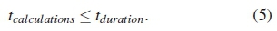
There are however still applications that require the same detection capabilities, but where processing time is of the utmost importance. A further constraint arises for these techniques if they are to be implemented on streaming digital media - only current and historic data is available to the algorithm. Both of these constraints are addressed by the real-time criterion as discussed in Section 3.2.

Due to the varying nature of videos, each available technique will perform differently based on the input data. In this investigation the sensitivity of one such technique, the Jensen-Shannon divergence, is evaluated for a generic set of test videos. The knowledge gained from this analysis provides a set of seed parameter values, as well as an understanding of the various parameters' effects on the algorithm when used in conjunction with streaming media.

 

2. LITERATURE OVERVIEW

Although a literature study of the latest video segmentation literature produced multiple documents pertaining to video segmentation, it was met with some confusion. While the term is technically applicable to all instances, it does cause some confusion with regards to the focus of the segmentation. Within the context of this article, the term video segmentation refers to segmentation of a video into the various segments from which it is comprised, by employing a shot boundary detector. There are however other forms of video segmentation used to segment the video in other contexts.

One such a video segmentation method is focused on the regions within frames - e.g. to generate a binary mask for a given target object in each frame [25]. While some of these masking-video segmentation methodologies can be employed to measure the consistency or presence of a target in a frame, which can be evaluated to detect a possible shot boundary, it generally comes at a price as it is computationally expensive. Similarly Caelles et al. discusses the semi-supervised video object segmentation regarding the separation of an object from the background in a video [7].

These masking-video segmentation methodologies face the same issues as the proposed shot boundary detector methodology - the efficiency of a segmentation technique may vary with the category or genre of the video being analysed [4]. Although the area of segmentation differs from what is addressed in this article, both are affected by the genre of the video being analysed. In order to mitigate this sensitivity as far as possible, the sensitivity of the proposed algorithm in this article is evaluated by using a multi-genre data set.

In some instances the term video segmentation is more focused on the physical data representing the video. Kalaiselvi et al. used the term video segmentation to describe the segmentation techniques pertaining to the data segmentation for cloud storage in [14].

While there are multiple techniques that are able to detect the various boundary frames between scenes, many of them rely on the whole video being available for a recursive analysis. One such an algorithm is employed by Sakarya et al. where the most reliable solution is evaluated with the first pass while other solutions are exploited in subsequent recursive steps [21]. While this approach can produce accurate results, it is in violation of the real-time constrains.

Similarly the term video temporal segmentation is used by e Santos et al. in [10] to refer to a video transition detection method. While the video segmentation method pertains to the detection of transitions, it does however also require the whole video to be available as they normalize their dissimilarity vector as well as employing a double-sided moving average window - i.e. using future frames.

Although the aforementioned video segmentation literature might be focussed on different segmentation contexts, many of them still share common shortfalls such as requiring the whole video to be available or the genre-sensitivity. While these shortcomings were taken into account, it was noticed that the majority of available literature does not expand on the sensitivity of the parameter values they employ. One such an example is the work presented by Widiarto et al. in [28] where they implemented a histogram based approach for video segmentation by calculating histograms for each of the RGB (Red-Green-Blue) color components of the video. There is however no information, nor justification provided as to the chosen threshold used in conjunction with the Euclidean distance metric which is calculated from the histograms. While the work presented in [28] utilises a video segmentation algorithm, the focus seems to be on subsequent processing of the video, with no useful information pertaining to the video segmentation algorithm.

Mentzelopoulos et al. also proposed an entropy based algorithm for key-frame extraction in [18]. While the algorithm performed very well when the background image was easily distinguishable from the objects, the performance dropped when transient changes were encountered.

While it is clear from the latest literature sources that there is still a need for video segmentation in all its variable contexts, the lack of parameter justification and the sensitivity thereof, makes it difficult to apply or predict the outcome of these algorithms on different types or sizes of videos. The aim of this paper is to provide parameter justification and a sensitivity analysis thereof to aid in the application of this video segmentation algorithm in different implementations and various video sets.

 

3. BACKGROUND

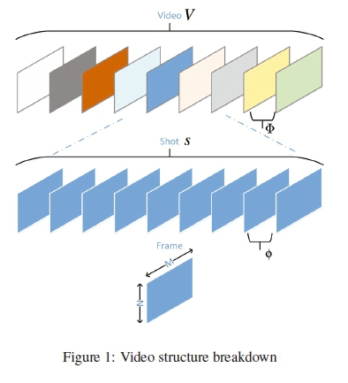
In order to understand and appreciate the functionality of a shot boundary detector (SBD), one has to understand the basic underlying structure of video files. Automatic shot boundary detection plays a pivotal role in completing tasks such as video abstraction and keyframe selection [8]. The ambiguous term video has its origin from the Latin word videre meaning 'to see' combined with the English word audio which refers to the process of hearing, ultimately forming a word that describes a coalesced union of audio and visual material known as video. For the purpose of this investigation, the term video will semantically refer to the visual aspect thereof.

3.1 Video structure

A generic video file V can be defined as a collection of various smaller sections called shots s:

These shots are defined as video segments that are visually contiguous and generally captured during a single take. This implies that although the visual content might be varying as is the nature of videos, the inter-frame variances φ should be small compared to the inter-shot variances Φ. The underlying structure of a shot consists of multiple sequential static frames f:

Each of these static frames can be represented by a M χ N matrix where each picture element (pixel) p_i,j can be addressed by its relative position in the frame by its co-ordinates i and j. In colour frames, each pixels has a multi-chromaticity value (RGB or CMYK (Cyan-Magenta-Yellow-Key (black)) color space) that defines the colour thereof. Similarly for grayscale frames, each pixel has a monochromatic value. This generic breakdown of the video structure is illustrated in Figure 1.

 

 

3.2 Shot Boundary Detection

Human beings are able to detect the boundaries between various shots due to cognitive analysis. However, computers lack the cognitive analysis capabilities of humans and thus need to analyse the video in a different manner.

A shot boundary can be defined as the break in visual continuity between two sequential shot sequences. In the simplest form, this boundary can be depicted as two sequential frames that contain drastically different visual content. This break in visual continuity can thus be detected by measuring the inter-frame variance between sequential frames. When the inter-frame variance between two frames is sufficiently larger than the preceding inter-frame variances, it can be an indication of a shot boundary. This variance will then be called an inter-shot variance.

Following this simple premise, a computer can then analyse videos and based on the results thereof, infer possible shot boundary locations. There are however numerous contributing factors that hamper the detection of boundaries.

Transitions: The transition between shots describe the way in which the shot boundary is implemented. There are two main categories of transitions used in videos: abrupt and gradual transitions. In the simplest form, a shot transition can be described as the visual manifestation of an abrupt change in visual content, hence called an abrupt transition.

In order to soften the visual discontinuity caused by a shot boundary, techniques can be employed to alter the frames surrounding the shot boundary. A basic gradual transition technique is called fading where the opacity or luminosity of sequential frames in the one shot is gradually decreased while the inverse is done on the following shot. A common example of such a fade is commonly referred to a as fade-to-black where the current shot is faded to a black frame.

The progress of video editing techniques have brought forth multiple transition techniques to create visually appealing shot transitions, but which tend to complicate the automatic detection thereof. These include transitions like:

• additive dissolve;

• cross dissolve;

• fade-to-black and fade-from-black;

• zoom in or out;

• slide;

• page peal;

• iris box.

and many other interesting transitions.

With the exception of dissolves and fade-to-black or fade-from-black, the other transitions are not generally encountered in general video sources such as television programs and movies. It is more commonplace in advertisements or presentation videos.

Detection Methodologies: The simplest method that can be employed with the goal of detecting shot boundaries is the comparison of successive frames. This can be accomplished by comparing the value of each corresponding pixel in both frames and calculating the difference thereof. In this case the difference D_n,n+1 will be the aforementioned inter-frame variance φ_n,n+1.

If the total difference between the two frames are above a certain threshold τ, it might be possible that a shot boundary has been detected:

It is easy to see how this pixel based method can become computationally expensive as well as very susceptible to noise since each pixel is evaluated as a singular entity [26]. Alternatively the pixels can be analysed as groups of entities, allowing for a reduced impact due to noise and camera motion [12].

Lefevre et al. reviewed multiple video segmentation techniques in [15], concluding that inter-frame difference is indeed one of the fastest methods although it may be characterised by poor quality. On the other end of the spectrum are feature or motion based methodologies which are more robust, but are computationally expensive. Furthermore, some of the more robust techniques not only require the video as a whole to detect peaks in analysis outputs, but require training for the statistical learning methods. Since training can alter the output of the results depending on the training set used. Hence different instantiations could be subject to different results while using the same algorithm if trained using a different set. Thus the aforementioned arguments reinforce the notion to opt for a fast procedure based technique. One such a technique is the histogram based Jensen-Shannon divergence. A previous investigation by De Klerk et al.

[19] revealed the viability and usefulness of this technique as a boundary detection algorithm.

Real-time: The concept of real-time is a fairly relative one. In this context the term does not refer to the validity of time, but rather to a relational expression. For the purpose of this investigation, the term real-time will be defined as the analysis time domain where the time required for all computations t, is equal to or preferably less than the actual playback duration t_duration of the video being analysed

Another constraint imposed on the analysis techniques pertaining to the streaming media aspect, is that the analysis technique will only have historic data available to perform the analysis. This becomes a notable factor when calculating the aforementioned threshold, as some traditional techniques rely on a global threshold calculated from the whole composite video which is now unavailable.

3.3 Jensen-Shannon Divergence

The Jensen-Shannon Divergence algorithm provides a means to determine the inter-frame variance φ between consecutive frames. This in turn can be used to detect if these frames constitute a shot boundary. Thus, a generalised form of equation 4 can be given as:

As the name suggests, the JSD algorithm is a combination of the Shannon's entropy and the Jensen inequality.

In 1984, Claude Shannon defined information measures for instance, mutual information and entropy. The Shannon entropy [23] is a method used in information theory to express the information content, or the diversity of the uncertainty of a single random variable, i.e. a measure of information choice and uncertainty [11].

The Shannon entropy function H of the probability distribution P = (p₁,p₂,p₃,...,p_n) consisting of n possibilities in the distribution is calculated by:

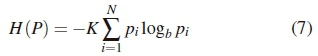
where K is a positive constant [17] and b denoting the logarithmic base [22]. In essence, this entropy measure can be explained as the measure of uncertainty to predict which probability in occurrence will be encountered.

The other part of this technique relies on the Jensen's inequality measure as was proposed by Johan Jensen in 1905 in the paper Sur les fonctions convexes et les inégalités entre les valeursmoyennes [13]. Fundamentally, the Jensen-inequality states that if a given function g is convex on the range of a random variable Y, then the expected value E of the function will be greater than or equal to the function of the expected value:

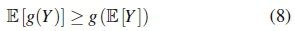
where the variance will always be positive. This property can be illustrated by evaluating the Jensen-inequality for the convex function g(y)= y². This will always be positive since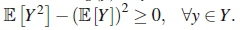

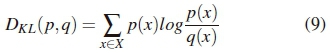
In order to understand the relevance of the Jensen-inequality to the functionality of boundary detection, a specialised version of the Shannon entropy is however required, namely relative entropy. Relative entropy is a further application of Shannon's entropy which can be used to quantify the distance between two probability distributions. This relative entropy, also referred to as the Kullback-Leibler distance, is denoted by D_KL(p, q) and calculates the distance between two probability distributions p and q that are defined over the alphabet χ:

where x e χ. By following the conventions, as used by [11] and [24] that

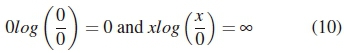
if x > 0, it becomes apparent from equation 9 that the relative entropy satisfies the information inequality or divergence:

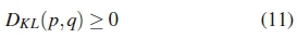
if and only if p = q. This implies that only when both distributions are identical, the Kullback-Leibler distance can be zero. For all other instances it will be greater than zero. This information inequality or divergence, is sometimes referred to as the information divergence [11] and is later used with the Jensen inequality, hence becoming the Jensen divergence.

The integration of the entropy measures from Shannon with the inequality measure of Jensen, in effect, enables the measuring of the expected entropy of the probability, which will be greater than or equal to the entropy of the expected probability.

Thus, by combining Shannon's entropy with Jensen's inequality, one is left with a commonly used index of the diversity of a multinomial distribution. Consider a multinomial distribution p =(p₁,..., p_n), where each p_i≥ 0 and the total sum of the distribution is Σ p_i = 1. Burbea et al. expressed the concavity of the Shannon entropy provides a decomposition of the total diversity in a mixed distribution as:

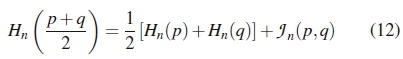
in [6]. The average diversity within the distributions is represented by the first component  in equation 12, while the latter component is called the Jensen difference.

The Jensen difference J_n(p, q) corresponds to the Shannon entropy H_n (p) and can be expressed as:

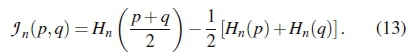
The Jensen difference is non-negative and vanishes if p = q and thus provides a natural measure of divergence between the two distributions [6] as with the relative entropy in equation 11.

Thus, by combining the entropy calculation with the Jensen inequality measure between two consecutive frames' histograms as derived by Qing Xu [27], the JSD equation is produced:

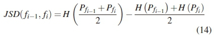
where f_i-1is the previous frame and f_ithe current frame. A measure is created as to how far the probabilities are from their likely joint source, equalling zero only if all the probabilities are equal. The probabilities of the frames are respectively  and  . The aforementioned probabilities are calculated from the applicable frames' histograms as expressed in equation 15:

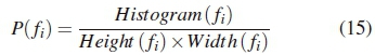
where the histogram of each color component is divided by the number of pixels in that frame f_i. The total number of pixels is calculated by multiplying the number of horizontal pixels by the number of vertical pixels in the frame.

3.4 Threshold

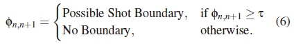
The Jensen-Shannon divergence, as expressed in equation 14, provides a unique inter-frame variance measure. In order to ascertain if the inter-frame variance constitutes a shot boundary, we refer back to equation 4. In order for a metric to be effective in detecting a shot boundary, it has to be evaluated against a representative threshold τ.

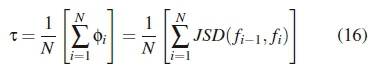
Some existing techniques calculate the inter-frame variance between each frame in the video and then calculate the average thereof:

where N Є Z represents the total number of frames within the video and the inter-frame variance φ is the JSD( f_i-1, f_i) calculated by equation 14. It is important to note that if the inter-frame variance φ; = JSD(f_i-1,f) where i = 1 will result in a very large value as the zero-frame f₀ does not exist and is generally represented by a black frame. This is however not the case when encountering a fade-from-black transition at the start of the video due to the gradual change - low inter-frame variance.

Although this type of global thresholding allows for a well-represented threshold, it does however not conform to the real-time criteria as set forth in subsection 3.2. This short fall can be overcome by calculating a moving average from a selection of the last preceding frames against which the inter-frame variances can be evaluated. This auto-adjusting threshold τ can be represented by:

where ω is the number of preceding frames to be evaluated for the moving average. The value of ω will be evaluated in section 5.1.

 

4. METHODOLOGY

4.1 Simulation Platform

A simulation platform was created in Visual Basic that allows various video formats to be analysed. At the core of this simulation platform is EMGU CV (version 3.0.0.2158). EMGU CV is a cross platform .Net wrapper for OpenCV (Open source computer vision). This is a library consisting of a multitude of programming functions aimed at computer-vision applications [1].

In order to simulate the channel used by streaming media applications, the simulation platform loads a video and supplies the algorithm currently being evaluated with a sequential stream of video frames. Once the frames have been evaluated, they are discarded to free up memory. Research has shown that the compression and encoding properties of certain video streams and files can be exploited to further increase the processing speed of the algorithm in certain instances [9]. Despite this advantage, it was decided that the algorithm being evaluated in this platform, be evaluated at face value when supplied with the sequential frames excluding any accompanying compression and encoding information.

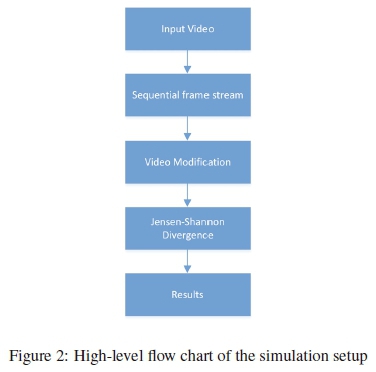
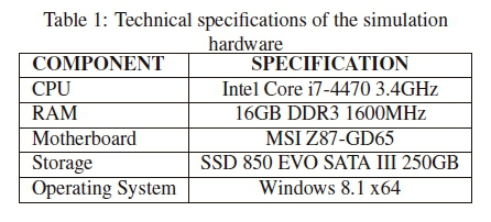
In order to evaluate the processing duration of the algorithms, the logical flow, as illustrated in figure 2, was implemented to run linearly as a single thread. In doing so, the efficiency of the technique is evaluated and not merely the multi-threading capabilities of the hardware platform. Specifics of the hardware used in the analysis is summarised in table 1.

 

 

 

 

4.2 Simulation setup

Lienhart et al. performed a comparison of a few automatic shot boundary detection algorithms in [16]. The main focus of the algorithms in this comparison was the accuracy thereof with no mention of the processing speed or duration. Due to the real-time criteria, the execution duration of the technique has to be considered alongside the accuracy thereof.

It is clear from equation 14 that Jensen-Shannon divergence has limited parameters for optimisation. The only variable aspects are the probabilities calculated from the frames. Hence the best area for evaluation and optimisation of the technique can be identified as the manner in which this inter-frame variance is compared - i.e. the threshold. Thus the evaluation of the Jensen-Shannon divergence technique's efficiency, as a shot boundary detection technique, is accomplished by performing a basic sensitivity analysis of the following parameters pertaining to the threshold:

• Auto-adjusting threshold frame count (ω);

• Minimum threshold scalar (η);

• Average threshold scalar (α);

• Resize factor.

During the threshold comparison, the auto-adjusting threshold expressed by equation 17 is multiplied by the average threshold scalar α allowing the operator to dictate how much greater the inter-frame variance must be to be classified as a shot boundary. This evaluating threshold Τ has a further constraint imposed where a minimum threshold is used to evaluate the inter-frame variance if the evaluating threshold was too low:

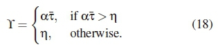
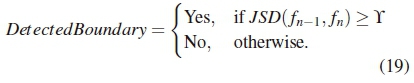
Thus the final outcome of the boundary detection test is given by:

4.3 Data

Due to the infinite video possibilities that can be encountered, a diverse collection of videos were chosen to evaluate the video segmentation technique. These videos encompasses various transitional effects as well as various sizes and frame rates. In order to establish a baseline, a few test videos were created in Adobe Premier where the same two shots were joined using various transitions. Two video segments created from the Windows 7 sample video named Wildlife was subjected to various transitions as mentioned in section 3.2. The videos were encoded using the Flash Video format (.flv), using a framerate of 29.97 frames per second (FPS) with a resolution of 1280 χ 720. The shot boundary between the two segments was created with the second segment starting on frame 60, hence a hardcut shot boundary. All the other transitions started on frame 49 and ended on frame 73. Some actual advertisements containing rapid moving scenes, multiple transitions and lens flares were also evaluated such as The World of RedBull TV Commercial [3].

4.4 Video Modifications

The video modifications mentioned in figure 2 pertains to the colorspace as well as the size of the video. All the videos used in the analysis are natively colour videos in the RGB domain. This specific implementation of the Jensen-Shannon divergence utilises only a single representative information source to calculate the inter-frame variance. This implies that all input videos frames are converted or flattened to the monochrome colorspace. This allows the grayscale luminescence to be used as the basis for the probability distribution.

The resize factor (RF) represents the scalar according to which the original frame is resized using bilinear interpolation with the help of the Inter.CV_INTER_LINEAR function [2].

4.5 Evaluation Metrics

Various metrics were employed to evaluate the effectiveness of the shot boundary detection algorithm that was evaluated.

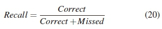
Recall: Recall rates provides a ratio of the number of relevant shot boundaries (correct detection) to the total number of relevant shot boundaries in the video, as expressed in equation 20.

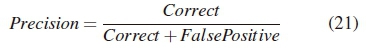
Precision: The precision rates of the algorithm provides the ratio of relevant shot boundaries to the total number of irrelevant shot boundaries (false detections) retrieved, as expressed in equation 21 [20].

Execution time: The execution time of each analysis will be recorded alongside the recall and precision rates thereof. This will help to justify a trade-off analysis between the technique parameters in terms of accuracy versus the execution time required. This becomes particularly important for "real-time" applications.

The execution time includes the following:

• Opening the video and reading the frames as they are required;

• Converting from RGB to monochrome where required;

• Resizing of the incoming frames where required.

 

5. RESULTS

The analysis results in this section is grouped according to the parameter under investigation. The majority of all the graphs in this section is representative of the average values produced by each of the 31 test videos. The influences of video resizing is incorporated in the other analysis.

5.1 Auto-adjusting threshold frame count

The first parameter that was investigated is the number of frames used by the auto-adjusting threshold as this outcome was used as an input parameter for the subsequent analyses.

While most of the test videos resulted in very good recall and precision rates, other, especially some videos with abnormal gradual transitions, performed poorly. In order to provide a representative sample, the average recall rates were calculated of all 31 videos with an accompanying standard deviations. The same was done with the precision values. Further investigation indicated that there were 5 specific test videos which exhibited poor recall values,. This was due to the slow changing nature of the videos e.g. an advert with a static background where the biggest changes were contributed by some animated text (small percentage of the frame). These results were still incorporated into the analysis.

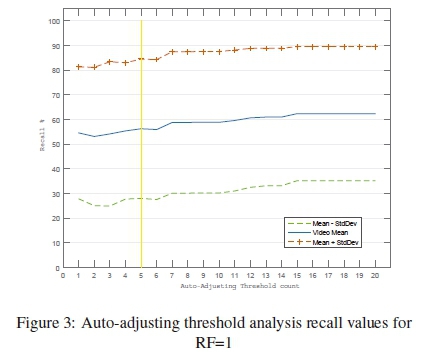
The average recall response of the system for a resize factor (RF) equal to 1 is illustrated in figure 3 which seems to be increasing fairly linearly with regards to an increase in the number of frames.

 

 

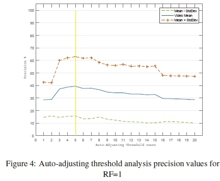
This is however not the case for the accompanying precision response as seen in figure 4. An initial increase in the precision rate is observed but then followed by a steady decline. A maximum precision response was observed at a frame count of 5.

 

 

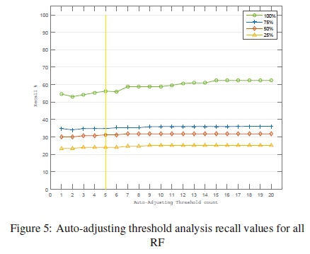
Similarly the recall behaviour for the other resize factors follow the same trend seen in figure 5 with increasing linear patterns but lower average values.

 

 

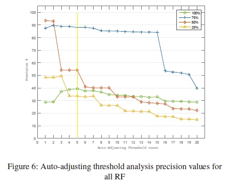
Logic infers that the precision values will also follow suit.

Generally this assumption is correct - all the resize factors follow a steady decline, however the concave form with a local maximum is not as clear. There is an anomaly with regard to RF = 75% as shown in figure 6. The precision rates for this RF is noticeably higher than the other RF values. The possible cause for this might be attributed to the bilinear resizing algorithm that is applied to the frame. By resizing the frame, the image is condensed, but at RF=75% still retains a large amount of unique information for an inter-frame variance to be calculated.

 

 

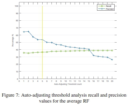
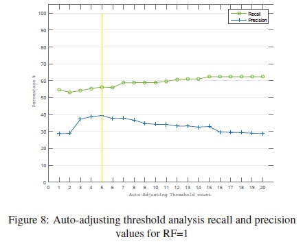
The ideal frame count will result in maximum recall and precision values, hence the intersection of the two graphs as seen in figure 7, which represents the average recall an precision values across all RF values. The intersection is visible at a frame count ω = 15 with an average recall and precision rate of approximately 39%. Due to the aforementioned anomaly at the 75% resize factor, the intersection point for this RF was specifically evaluated. Although not indicated on figure 7, the raw data indicated that the point of intersection for RF=75% was found to be at a frame count ω = 21 with an average recall and precision rate of approximately 35%. These rates are however deemed too low. The recall and precision rates for RF=100% is shown in figure 8 with a recall rate of 67% and a precision rate of 40% at a frame count ω = 5.

 

 

 

 

5.2 Average threshold sensitivity

The second parameter to be evaluated was the average threshold sensitivity while using the previously calculated frame count ω = 5. The recall rates obtained show a quick decline before appearing to stabilise as seen in figure 9.

 

 

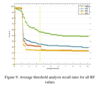
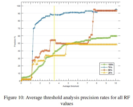
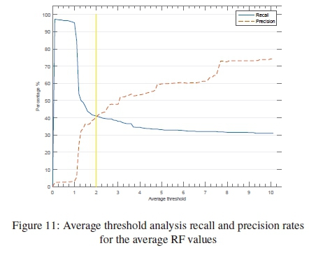
The precision rates present with a large initial increase that appears to level off at higher threshold levels shown in figure 10. The intersecting point for RF=75% is situated at α ≈ 1.2 which results in recall and precision rates of approximately 49%. The best rates are obtained where RF=100% where α = 5.7 resulting in recall and precision rates of 51%. The intersecting point when evaluating the average for all RF values is located at α = 2 with recall and precision rates of approximately 41% as illustrated in figure 11.

 

 

 

 

5.3 Minimum threshold sensitivity

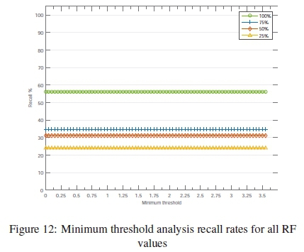
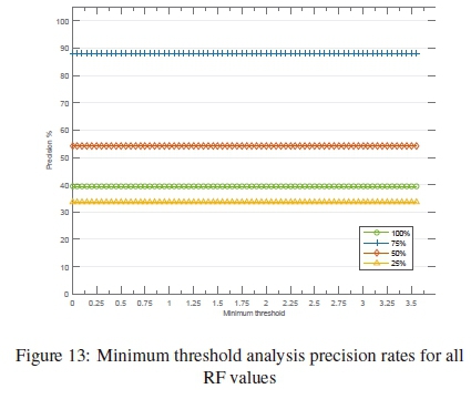
The sensitivity of the detection technique to variations in the minimum threshold was analysed while using an average threshold α = 3.5 and a frame count ω = 5. This analysis indicated that any variations in the minimum threshold 0 ≤ η ≤ α does not relate to any change in the recall and precision rates for any RF as shown in figures 12 and 13.

 

 

 

 

5.4 Analysis duration

The analysis durations for the auto-adjusting threshold frame count analysis is illustrated in figure 14 from which it is evident that the analysis duration follows a fairly linear pattern, where ω > 2, with the exception of the initial threshold value of RF=1.

 

 

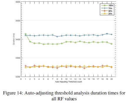
The same linear behaviour is encountered during all the other investigations. The general trend for all parameter analyses, as seen in figure 15, indicates that the RF = 75% actually took the longest to complete.

 

 

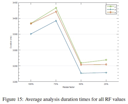
With regard to the real-time component, the maximum average duration encountered at RF = 75% at approximately 3435ms. When comparing this maximum to the average duration of the test video 9985ms, it is clear that the real-time criteria will be met as the analysis duration is at least 2.9 times faster than the playback duration. In order to ensure that unbiased timing was achieved, each value for each parameter under investigation was analysed 10 times with the average thereof taken as the analysis duration for that instance.

 

6. CONCLUSION AND RECOMMENDATION

The Jensen-Shannon divergence proved to be a technique capable of detecting shot boundaries with fairly good recall and precision rates. The analysis duration of the technique more than satisfied the real-time requirements while using only the historic (received) data for calculations.

It is important to note that the average CPU usage was, on average 35%, as well as the average RAM usage at 33% throughout the analysis. This indicates that the timing for the analysis is representative of the actual execution and not perplexed by the system bottlenecking by e.g. caching to a page file if the RAM was filled.

The results indicate that the RF = 75% has some outliers with regards to the α- and ω precision rates as well as longer execution times.

A finer resolution analysis of the resize factor would be beneficial to pinpoint the optimal RF in terms of optimal recall and precision rates while keeping the analysis duration as low as possible.

The optimal parameters based on the simulation results contained in this article is as follow:

• ω = 5;

• α = 5.7;

• η =No-effect η = 0.

Throughout the analysis a noticeable abrupt decline in precision rates was observed at ω = 5, which warrants some further investigation.

 

ACKNOWLEDGMENTS

I would like to thank Prof. W.C. Venter for the assistance during this investigation as well as Prof. A.J. Hoffman for the continued financial contribution towards the project.

 

REFERENCES

[1] Open source computer vision library [online]. URL: http://opencv.org/about.html.

[2] Opencv geometric image transformations [online]. URL: http://docs.opencv.org/3.1.0.

[3] The world of redbull tv commercial 2013 [online]. URL: https://www.youtube.com/watch?v=XSFIELPSGnU.

[4] H. Aditya, T. Gayatri, T. Santosh, S. Ankalaki, and J. Majumdar. Performance analysis of video segmentation. In Advanced Computing and Communication Systems (ICACCS), 2017 4th International Conference on, pages 1-6. IEEE, 2017.

[5] A. M. Amel, B. A. Abdessalem, and M. Abdellatif. Video shot boundary detection using motion activity descriptor. arXivpreprint arXiv:1004.4605, 2010.

[6] J. Burbea and C. R. Rao. On the convexity of some divergence measures based on entropy functions. Technical report, DTIC Document, 1980.

[7] S. Caelles, K.-K. Maninis, J. Pont-Tuset, L. Leal-Taixe, D. Cremers, and L. Van Gool. One-shot video object segmentation. In CVPR 2017. IEEE, 2017.

[8] C. Chan and A. Wong. Shot boundary detection using genetic algorithm optimization. In Multimedia (ISM), 2011 IEEE International Symposium on, pages 327-332. IEEE, 2011.

[9] M. Chunmei, D. Changyan, and H. Baogui. A new method for shot boundary detection. In Industrial Control and Electronics Engineering (ICICEE), 2012 International Conference on, pages 156-160. IEEE, 2012.

[10] A. C. S. e Santos and H. Pedrini. Shot boundary detection for video temporal segmentation based on the weber local descriptor. IEEE International Conference on Systems, Man, and Cybernetics, pages 1310-1315, October 2017.

[11] M. Feixas, A. Bardera, J. Rigau, Q. Xu, and M. Sbert. Information Theory Tools for Image Processing, volume 6. Morgan and Claypool Publishers, 2014.         [ Links ]

[12] U. Gargi, R. Kasturi, and S. H. Strayer. Performance characterization of video-shot-change detection methods. Circuits and Systems for Video Technology, IEEE Transactions on, 10(1):1-13, 2000.         [ Links ]

[13] J. L. W. V. Jensen. Sur les fonctions convexes et les inegalites entre les valeurs moyennes. Acta Mathematica, 30(1):175-193, 1906.         [ Links ]

[14] N. Kalaiselvi, A. Gayathri, and K. Asha. An efficient video segmentation and transmission usingcloud storage services. In Signal Processing, Communication and Networking (ICSCN), 2017 Fourth International Conference on, pages 1-6. IEEE, 2017.

[15] S. Lefevre, J. Holler, and N. Vincent. A review of real-time segmentation of uncompressed video sequences for content-based search and retrieval. Real-Time Imaging, 9(1):73-98, 2003.         [ Links ]

[16] R. W. Lienhart. Comparison of automatic shot boundary detection algorithms. In Electronic Imaging'99, pages 290-301. International Society for Optics and Photonics, 1998.

[17] M. Menendez, J. Pardo, L. Pardo, and M. Pardo. The jensen-shannon divergence. Journal of the Franklin Institute, 334(2):307-318, 1997.         [ Links ]

[18] M. Mentzelopoulos and A. Psarrou. Key-frame extraction algorithm using entropy difference. In Proceedings of the 6th ACM SIGMM international workshop on Multimedia information retrieval, pages 39-45. ACM, 2004.

[19] M.G. de Klerk and W.C. Venter and A.J. Hoffman. Digital video shot boundary detector investigation. In Southern Africa Telecommunication Networks and Applications Conference (SATNAC) 2014, pages 105-110, http://www.satnac.org.za/, 2014. Southern Africa Telecommunication Networks and Applications Conference (SATNAC).

[20] V. Raghavan, P. Bollmann, and G. S. Jung. A critical investigation of recall and precision as measures of retrieval system performance. ACM Transactions on Information Systems (TOIS), 7(3):205-229, 1989.         [ Links ]

[21] U. Sakarya, Z. Telatar, and A. A. Alatan. Dominant sets based movie scene detection. Signal Processing, 92(1):107-119, 2012.         [ Links ]

[22] T. D. Schneider. Information theory primer, 1995.

[23] C. E. Shannon. A mathematical theory of communication. SIGMOBILE Mob. Comput. Commun. Rev., 5(1):3-55, jan 2001. URL: http://doi.acm.org/10.1145/584 091.5 84093, doi:10. 1145/584091.584093.         [ Links ]

[24] I. Spanou, A. Lazaris, andP. Koutsakis. Scenechange detection-based discrete autoregressive modeling for mpeg-4 video traffic. In Communications (ICC), 2013 IEEE International Conference on, pages 2386-2390. IEEE, 2013.

[25] C. Sun and H. Lu. Interactive video segmentation via local appearance model. IEEE Transactions on Circuits and Systems for Video Technology, 2016.

[26] A. K. Tripathi, U. Ghanekar, and S. Mukhopadhyay. Switching median filter: advanced boundary discriminative noise detection algorithm. Image Processing, IET, 5(7):598-610, 2011.         [ Links ]

[27] M. Vila, A. Bardera, Q. Xu, M. Feixas, and M. Sbert. Tsallis entropy-based information measures for shot boundary detection and keyframe selection. Signal, Image and Video Processing, 7(3):507-520, 2013.         [ Links ]

[28] W. Widiarto, E. M. Yuniarno, and M. Hariadi. Video summarization using a key frame selection based on shot segmentation. In Science in Information Technology (ICSITech), 2015 International Conference on, pages 207-212. IEEE, 2015.