Neural network fault diagnosis system for a diesel-electric locomotive's closed loop excitation control system

 

 

M. Barnard; TI. Van Niekerk

Department of Mechatronics, Nelson Mandela Metropolitan University, PO 77000 Port Elizabeth 6031, South Africa E-mail: s207073708@live.nmmu.ac.za, Theo.vanNiekerk@nmmu.ac.za

 

 

---

ABSTRACT

In closed loop control systems fault isolation becomes extremely difficult in the case of feedbacks being oscillatory due to corrupted signals or malfunctions in actuators. This paper investigates and highlights the development of an off-line fault detection and isolation system for the isolation of faults, which cause oscillatory conditions on a General Electric (GE) Diesel-Electric Locomotive's excitation control system. The paper illustrates the use of artificial neural networks as a replacement to classical analytical models used for residual generation. The artificial neural network model's design is based on model-based dedicated observer theory to isolate sensor, as well as component faults, where observer theory is utilised to effectively select input-output data configurations for detection of sensor and component faults causing oscillations. Residual Evaluation is done with the use of a moving average filter incorporated with the simple thresholding technique. The results indicated 100% accuracy for the detection and isolation of the component or sensor responsible for causing excessive oscillation in the excitation control system.

Key words: Neural Network Residual Generator, Artificial Neural Networks, Moving Average Filter, Simple Thresholding, Off-line Neural Network Model-Based Fault detection and Isolation.

---

 

 

1. INTRODUCTION

An unappealing characteristic of real world control systems is the fact that they are vulnerable to faults, malfunctions and unexpected modes of operations due to component and/or sensor failures. These failures affect operations in industrial plants negatively in terms of production or a plant's operating time.

In any production line, service centre or really any business, time plays a very important role. Time is the key factor which determines delivery and quality, as well as profitability. One of the key factors affecting the operating time of machinery is unscheduled breakdowns which in turn requires unscheduled maintenance. Within the maintenance environment, "fault isolation" time, which can be defined as the time taken to isolate a faulty component, can be considered one of the most important factors affecting production or a plant's operating time.

Owing to the increasing demands on the reduction of this time, research in the field of fault detection and isolation has received increasing interest over the years, especially in automated environments, which has led to a significant improvement in the process of fault detection and isolation, with a large reduction in the need for limit checking or trend analysis, which requires expert knowledge of systems, in order to perform fault detection and isolation [1, pp.22-23]. In order to avoid the heavy economic losses involved in halted production, due to the replacement of elements, parts and fault isolation, literature on methods to perform fault diagnosis are mostly aimed at performing fault detection and isolation with the use of model-based techniques, which are created with the use of analytical approaches. The problem with the analytical approach is that most industrial systems cannot easily be modelled due to their sheer size, complexity, unavailability of component data of the design, measurements being corrupted by noise and unreliable sensors within the control system. Owing to this, a number of researchers have focussed their research on the use of neural networks to produce models of industrial processes [2], [4], [5], [6], [8], [13]-[16], [19]-[23]. This is due to the fact that neural networks have the ability to filter out noise and disturbances, thus providing a stable and highly sensitive model of an industrial system without the use of a mathematical model.

This paper uses the above mentioned abilities of a neural network to model the closed loop excitation control system of a Diesel-Electric locomotive to enable the use of dedicated observer theory, which incorporates model-based fault detection and isolation, to detect and isolate oscillatory faults within the excitation system. The model design and development is done offline due to the nature of the locomotive's data acquisition system. Within this application the isolation of oscillatory faults are challenging due to all readings oscillating, as the control system tries to correct the error.

 

2. MODEL-BASED FAULT DIAGNOSIS USING NEURAL NETWORKS

When utilising neural networks to model a system, the problems associated with Fault Detection and Isolation (FDI) methods being sensitive to modelling errors, parameter variation, noise and disturbance, experienced with the use of mathematical models are eliminated or reduced as no mathematical model is needed. Figure 1 illustrates a general scheme of a model-based fault diagnosis system which utilises neural networks as replacement to mathematical/analytical models.

 

 

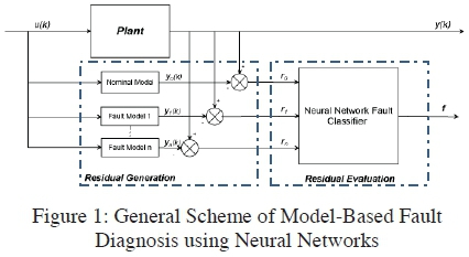
From Figure 1 it could be noted that there are different models running in parallel, where each model represents a class of the system or plant's behaviour. One model represents the system under normal operating conditions and each successive model thereafter represents a specific faulty condition.

The inputs u(k) are fed into each model where the models then outputs y₀(k), y₁(k),... y_n(k). These outputs are then compared to the plant's output y(k) to produce residual vectors [r₀,r₁,...r_n], which characterizes a suitable class of system behaviour [5]. This process is referred to as a residual generation function. The residual vector r is then transformed by a classification Neural Network to determine the location and time of the fault.

Neural networks can be successfully applied to perform fault diagnosis using different approaches. The different approaches can be defined as Pattern recognition and residual generation and evaluation where residual evaluation is basically a logical decision-making process which transforms quantitative knowledge into qualitative Yes-No statements. To perform the transformation from quantitative knowledge into qualitative statements, some measures need to be put in place to enable the FDI system to perform robust decisions. Thus in the field of residual evaluation, thresholding techniques are of great concern. The decision whether or not a faulty condition exists, can be a daunting task, as signals are corrupted by noise and disturbances. These corrupted signals have a huge impact on the magnitude of residuals.

In theory residuals in fault free cases should be close to zero and should be far from zero in the case of a fault. Thus some threshold value is needed to determine whether a residual value indicates a fault or not [8]. The challenge is in selecting a threshold value which is not affected by corrupted signals, but is still large enough to avoid false alarms, but small enough to still be sensitive to faults to prevent non-detections [8]. There exist a number of different methods to perform the decision making function in residual evaluation. Methods used are Neural Network Classifier, Neural Networks, Simple Thresholding, adaptive thresholding, moving average filters and statistical decision making theory [5] , [12].

 

3. OBJECTIVE

Currently isolating oscillatory faults occurring on the D34 class Diesel-Electric Locomotive's excitation system can take up to three hours. The reason for the large amount of time spend, is due to the fact that the current control system, does not perform fault detection and isolation for oscillatory control loop faults. Owing to this, the method followed to isolate faults is by elimination of possibilities.

This method eliminates the possible faulty components, one at a time on the locomotive, by replacing each component which has an impact on the excitation control loop, with a new one. The method is effective but takes up a lot of time, due to the location, as well as the structure of the components.

With time being one of the most important aspects within the maintenance environment and especially in the field of fault isolation, it was of great importance to research a method, which facilitated faster fault isolation on the excitation system of the locomotive.

In order to achieve this, design and development of a software-based fault detection and isolation system, to be used on the D34 Class Diesel-Electric locomotive's excitation control system for the detection and isolation of oscillatory faults was needed.

The software based FDI system would be an off-line data driven approach which utilizes feedforward neural network models to generate residuals. The residuals would then be evaluated against a threshold value, calculated with the aid of a moving average filter and simple thresholding.

The overall objective was to design and develop a software user interfacing program which could be coupled to the locomotive's control system to provide FDI on oscillating faults. The FDI system had to utilize a bank of nominal models of the system with dedicated observer configurations for the isolation of sensor and or component faults. The main difference between the general scheme and the applied FDI system is the use of only nominal models.

 

4. SYSTEM DEVELOPMENT

Figure 2 highlights the developed principle of operation of the FDI system used on the excitation closed loop control system on the locomotive. From the figure it could be noted that the FDI system is based on a dedicated observer scheme and therefor two separate banks of observers were utilised, one for the detection of sensor faults and the other for component faults.

 

 

The system works on the following basic concept; first the model outputs are compared with those of the system to generate residuals. These residuals will then be evaluated in a residual evaluation process. This process is indicated as component failure analysis in Figure 2. A count is made of how many times the residual for a specific reading exceeds a threshold value, where the highest number indicates the highest probability for the cause of the oscillation. With the possible cause isolated a neural network model is then selected in order to determine whether the fault is caused by a sensor failure. This process is illustrated as sensor failure analysis in Figure 2. The same evaluation process is followed as in the first step. The end result uses qualitative reasoning to determine whether the fault is a sensor or component failure.

4.1 Residual Generator

The principle of operation of a residual generator was discussed in section 2, where it was mentioned that the residual generator's output was the difference between a measured signal and a model's output. A number of quantitative model-based residual generation techniques exist where parameter estimation, parity equations, observers and the neural network residual generator was highlighted in [1], [3] and [5]. Isermann [1] highlights a number of real world applications and implementations of parameter estimation, parity equations and observers. Patan [5] shows the use of neural network residual generators in the fault diagnosis of technical plants.

Observer Model-based fault detection systems have been successfully implemented in a number of applications [9], [10], [11]. The method allows for the detection of actuator as well as sensor faults and has different configurations for the detection of sensor and actuator faults.

In a dedicated observer scheme several observers constitute a bank of reduced order observers, where for the detection of sensor faults each observer uses all the inputs and just one output to detect faults. Here the number of observers equals the number of outputs which is also equal to the number of sensors [7]. For the detection of actuator faults, each observer uses one input and all outputs. The dedicated observer scheme allows for the localization of multiple faults for either sensor or actuator faults [7].

Owing to this the input-output configuration of the training data to be used for training a neural network model as a dedicated observer is different for each sensor as well as for actuator faults.

 

5. MODELLING

One of the most important factors associated with a model-based fault detection and isolation system is the accuracy of the model. An artificial neural network provides an alternative to the classical approaches, but some knowledge of the system is needed to effectively develop an accurate model of the system. Thus for this application a mathematical analysis of the excitation system was done to determine dependencies. These dependencies provided the authors with knowledge of the system in terms of cause and effects. It also provided an insight into whether the system had linear tendencies which had an impact on the size and topology of the neural network [18].

5.1 Artificial Neural Network

Artificial neural networks have the ability to extract patterns and detect trends by deriving meaning from complex, incomplete or imprecise datasets. These datasets are usually too complex to be analyzed by either humans or conventional computer techniques. A supervised neural network which is trained on a set of data can be used to approximate an output for a set of inputs, which was not in the training set. Thus the neural network could be considered an expert on the dataset which it has learned. It is this type of neural network training which was utilized in the development of dedicated neural observer model for the detection and isolation of actuator as well as sensor faults. The application and availability of data is of utmost importance when selecting a neural network and analysis done on the locomotive's data acquisition abilities indicated that only recorded data could be obtained from the locomotive, thus rendering online fault diagnosis impossible. It was also found that the Original Equipment Manufacturer's controlling software was copyright protected and did not allow any online interface whatsoever. The recording function of the locomotive's software provided data on the nominal operation of the excitation control system and was perfect for the use of training data. Today a number of different neural network structures exist but for this application a feedforward neural network will be used [18].

5.2 Feedforward Neural Network Design

A feedforward neural network consists of three layers, namely: input, hidden and output layers which form what is known as a layered network. The layered network has feedforward connections from the input layer to the hidden layer, which is then in turn connected to the output layer which displays the result. The term feedforward is used to indicate that the network operates in one direction and does not have any feedback loops. Figure 3 illustrates a multi-layered feedforward neural network (FFNN). Here it can be seen that the network consists of three layers as mentioned in the above section (an input layer, a hidden layer and an output layer). It should be noted that a FFNN can have more than one hidden layer [18].

 

 

The three layers serve the following functions: the input layer receives the user input or data input from a source; each hidden layer processes the input layer's data net sum as well as its bias. Then it runs it through an activation function. No node on the hidden layer is interconnected; each output layer neuron then receives the data input from each individual hidden layer neuron, to compute the net sum plus bias, before calculating the result by passing the net sum through an activation function.

Model Input-Output Configuration

As mentioned previously a dedicated observer scheme for the detection of actuator and sensor faults was used to provide an accurate FDI system capable of detecting sensor as well as actuator faults. Figure 4 shows the input-output configuration for the detection of actuator faults. Here it could be noted that the input-output configuration satisfies the dedicated observer theory with regards to detecting faults in actuators.

 

 

For the detection of sensor faults an additional input-output training data set is needed. Mhamdi, Dhouibi, Liouane and Simeu-Abazi [7] describes an observer scheme for the detection of sensor faults as an observer which constitutes a bank of observers which receives all inputs and produces only one output, where the number of observers is equal to the number of sensors. Using this principle for the detection of sensor faults, the inputs and targets need to be different, thus indicating that additional observer models are needed, hence neural networks. In this case the number of additional neural networks is equal to 6, where all other measurements are used to predict a single sensor measurement.

It is these input-output configurations as illustrated in Figure 4 and 5, which were used as input and target data configurations to train a bank of neural network models to be used as residual generators.

 

 

Neural Network Architecture

In any artificial neural network the selection of an appropriate network model is of utmost importance, where the success of the network depends on the proper configuration of the network model. However the selection of a proper network configuration is more challenging due to the absence of generalized rules for defining a suitable network configuration. Thus it is difficult to define the number of hidden layers, hidden nodes and learning rate.

Number of Hidden Layers

When considering the number of hidden layers, it is important to realize that the more hidden layers are used, the more feedforward calculations are needed and hence the more computational time is needed. As noted in the above section, it is important to note that the simplest NN construction is always the best to use if it provides similar results to those of larger network constructions. Another important aspect to consider is the use of more hidden layers which has the disadvantage of reduced ability to generalize from unseen patterns outside of the training set [24].

In determining the number of hidden layers, it has been shown that one hidden layer neural network is sufficient to uniformly approximate any continuous functions [24]. Therefore, a single hidden layered neural network with tan-sig activation function was used. The tan-sig activation function has the characteristics of removing noise from a data set. [25]

Number of Hidden Layer Nodes

The number of hidden layer nodes can be determined from scratch through experiments, with the classical trial and error method. Engelbrecht [17] stated that if several network architectures fit a training set equally well, then on average the simplest one will give the best generalization performance. Sietsma and Dow tested and confirmed this in their journal. Engelbrecht [25] presented a simple method to determine the optimum model by training a few different network architectures and then chose the one with the lowest generalization error as estimated by the generalised predicted error. Gao [18] provided an additional check to determine whether there are too few hidden units, by monitoring the training error. If the training error is large then more hidden units are needed. Thus it could be noted that when considering the number of hidden nodes, it is important to note that there is no definitive method for deciding a priori number of nodes. The number of nodes can be closely related to the complexity of the non-linearity of the function to be generated by the network. The same as with the number of hidden layers: if too many hidden nodes are used the network is prone to overfitting and if too few are selected the accuracy of the network is negatively impacted. Thus a general procedure for selecting the optimum number of nodes as used by Saravanan, Duyar, Guo and Merrill [22], which is also highlighted by Engelbrecht [17], is to start with a small number of nodes and increase the number of nodes up to the point that there is no significant change in the networks accuracy. This method was successfully implemented by Saravanan, Duyar, Guo and Merrill [22].

Gao [18] further indicated that when one hidden layer is used the number of nodes to be used should be equal to 20. Experiments were done using the above mentioned methods to find the optimum network structure. Table 1 below shows the results from varying the number of hidden layers:

 

 

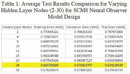
Results did however indicate the not all models performed best with the use of 20 hidden layer neurons, where some performed best with less and others with more hidden layers. It was also noted that the generalization ability with the use of hidden layer neurons not equal to 20 was not remarkably compared to the use of 20 hidden layer neurons structure.

5.3 Training

The accuracy of a neural network is determined by how effective it is trained. For this application it was found that the best training results was achieved with the use of the following training parameters: Dynamic learning Rate (Static Learning rate of 0.0001; Learning Rate Increment 1.0005; Learning Rate Decrement 0.007), Tan-Sig activation function, Z - scaling of the Inputs and Outputs, Static Momentum term of 0.9, Mean Absolute Error as the objective function, gradient descent optimization training algorithm and different hidden layer nodes for each neural observer models.

Each training process consisted of training each neural network 30 times and selecting the best generalization results. Table 2 below indicates the errors and training performances of each neural observer model.

 

 

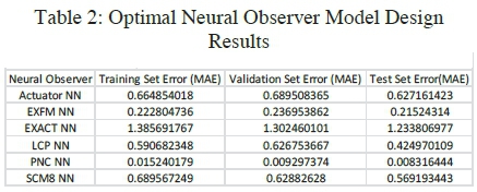
When comparing the model outputs with that of the locomotive's output it was noted that the overall performance of the neural network models were of high standard and sufficient to be used as residual generators.

The neural network models could correctly estimate the measured outputs with the following accuracy:

• Exciter Field Current Module (EXFM) - 91.5%

• Exciter Armature Current Sensor (EXACT) -98.06%

• Load Control Potentiometer (LCP) - 94.09%

• Power Notch Command (PNC) - 99.71%

• Engine Notch Command (ENC) - 98.51%

• Alternator's Voltage Sensor (SCM8) - 94.31%

From this it could be noted that the overall performance of the neural network models was satisfactory and could be used as a model in the model-based fault detection system.

 

6. RESIDUAL EVALUATION DESIGN

Any Model-Based fault detection system, whether analytical, artificial neural network based or fuzzy logic, consists of a residual generation process and a decision-making process, where the residuals are evaluated to make a decision whether or not a fault occurred. The decision-making process, is responsible for alerting a user of the occurrence of a fault.

Residual evaluation can thus be described as a logical decision-making process which transforms quantitative knowledge into qualitative Yes-No statements. To perform the transformation from quantitative knowledge into qualitative statements, some measures need to be put in place to enable the FDI system to perform robust decisions.

In this paper simple thresholding in conjunction with a moving average filter was used to determine threshold values.

6.1 Moving Average Filter

The generated residual, can be filtered with the use of a moving average filter, as to sufficiently dampen the residual noise [13, p.47]. The residual can then be expressed as follows:

 

 

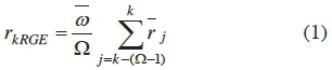
Where the arithmetic mean is chosen as the average and the weighted moving average of the past Ω residuals

generated, ω is equal to a user defined weight and r_krge is the residual generated at sample instant k . Now the generated residual can be evaluated with the use of a predefined threshold value. The moving average method is basically a moving average filter which filters out noise from the generated residual [13, p.47].

The degree of smoothing is determined by the number of points specified by Ω . A sample number (Ω) of 5 samples were used for smoothing the residual which consisted of 145 samples per locomotive recording, but with the use of the filter specified above, the total number of usable samples drops to 140, due to the filter being a forward moving average filter. Figure 6a and b below shows an example of the effect of using the moving average filter on the scaled residuals generated for the EXACT.

 

 

 

 

It could be noted from the figure above that the moving average filter, removes most of the noise in the residual, which makes thresholding calculation easier and minimizes the possibility of false alarms due to noise.

The filtered residual was then used to calculate a threshold value with the use of the simple thresholding technique.

6.2 Simple Thresholding

Simple thresholding is one of the simplest methods used for residual evaluation. The theoretical analysis of a healthy system is defined as follows: if the residual generated is smaller than a threshold value, the process is considered healthy, otherwise it is faulty. In theory a fault-free case refers to a condition in which the residual value is zero. However, in practice this is not feasible due to modelling errors and noisy signals; thus thresholds need to be larger than zero to prevent false alarms. In order to select a threshold range, let's assume that a residual satisfies the following:

 

 

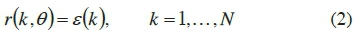
Where ε(k) is equal to N(m, v), which are random variables with a mean value m and standard deviation v . N specifies the number of samples which are used to calculate m and v. 0 represents the vector of the model parameters.

Residual evaluation is then done by comparing the absolute residual value and comparing it to its assigned threshold T . [6, pp.124-125] A diagnostic signal is then created and assigned a value, according to the following:

 

 

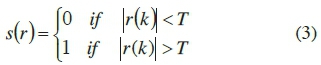
The diagnosis signal s(r) is assigned a value of zero if the residual's absolute value is less than the threshold T and one if it is greater. Thresholds can be calculated using the following threshold calculation. The threshold value is derived using Ç- standard deviation where the residual is assumed to be a random variable N(m, v) [5]. Thresholds are then calculated as follows:

 

 

Where m and v is defined as follows:

 

 

It is important to note that the above method works well and gives satisfying results when the residual is assumed to be normal. In order to determine whether residuals are normally distributed, a normality test required. In this paper the normality tests performed on the data was with the use of probability plots and the Chi-Square Goodness of fit functions.

Threshold Calculation for Component Faults

An important factor to consider when using the simple thresholding technique is that it can only be used with a high confidence level if the normality assumption is satisfied. Thus it is important to verify whether the filtered residuals are normally distributed and satisfy the normality assumption. Patan [5] stated that if simple thresholding is to be used on data which is not normally distributed, the system will tend to give more false alarms. Thus in this section normality tests will be done on the residuals observed from the component fault detection sections. The thresholds will then be calculated and tabulated for each observed measurement.

The component fault detection input-output configuration was highlighted in Figure 4, where 6 outputs were observed and compared to 6 neural network outputs, excited by two inputs. The difference between the neural network outputs and the observed outputs produces residuals and in this section analysis was done to verify whether the data is normally distributed to verify whether the simple thresholding technique could be applied with high confidence. Two main checks, namely: a probability plot and the Chi-Square Goodness of fit test were used to verify whether residuals were normally distributed. Results from the two tests indicated that the Power Notch Command input was not normally distributed; hence the simple thresholding technique could not be used to accurately calculate a threshold value. Owing to the function of the Power Notch Command, on the locomotive the threshold value was selected manually without the use of statistical techniques. With the normality tests done, the threshold values for the component or sectional fault isolation could be done, with the use of the simple thresholding technique. Table 3 below gives a summary of the threshold values calculated for each observed measurement.

 

 

It is important to note that these values were calculated from data obtained from the worst oscillating locomotive under normal conditions, meaning that the oscillations were still within limits.

Threshold Calculation for Sensor Faults

The sensor fault detection system is divided into 6 main groups, where each group constitutes a sensor reading validation. The sensor to be validated is selected from the highest failing component or sectional failure determined by the component failure analysis section. Sensor validation is done with the use of a dedicated observer scheme for the detection of sensor faults which has the effect that the configuration of the fault detection system is different in terms of its input-output configuration, when compared to component or sectional fault detection. As the configurations and errors of the neural network are different from that of the component analysis section, the residuals would also be different; hence normality tests on each sensor observers residual output was also necessary.

The results indicated that all the residuals were normally distributed except for the LCP's residual. Thus for the cases where the normality assumption could be made, simple thresholding was used to calculate a threshold value whereas with the LCP threshold value, system knowledge had to be incorporated and the effect of the LCP on the system had to be taken into consideration. Owing to the fact that the LCP reading had to be constant during notch 1 at 72Vdc, the neural network model's average testing error was added to a user defined maximum allowable residual of 3% to calculate the threshold. Table 4 below highlights the threshold values for each observed residual. The threshold was calculated from the worst yet in limit oscillating control system.

 

 

An important fact to remember is that the threshold value was calculated from filtered residual values which were filtered with the use of the moving average filter as indicated in section 4.2.

6.3 Fault Count Process

In its simplest form, the fault count process can be described as the number of times a residual exceeds a threshold value over a given time period. The reasoning behind using a count process is to eliminate false alarms caused by intermittent or abrupt signals by monitoring the system to see whether the fault persists.

The hypothesis seems to be simple and effective but does not work well with oscillatory faults within a closed loop control system, where the system's aim is to minimize the error between the output variable and the reference signal, causing all the sensor readings in the system to oscillate in excess of their threshold. It is for this reason that a simple count or penalty system could not be used for the isolation of faulty sensor or component faults causing oscillations.

The applied fault counting process is indicated below, where it could be noted that the count is done over M samples, where the count increment is based on the percentage of how far above the threshold value the residuals are. Thus if the residuals are far above the threshold it will give a 1 count otherwise it will increment with the percentage above the threshold.

 

 

Where:

R_n= Filtered residual,

M = Number of samples,

T (a) = Threshold for the observed signal, and

Count(a) = Fault count for the observed signal.

This method is based on the assumption that within a closed loop control system the greater the error the more system response is needed to correct the error, thus the residual which deviates the most from the norm, has a higher probability of causing the oscillation compared to that of a reading with a smaller deviation, which would cause a smaller error, hence less system response.

 

7. APPLICATION SOFTWARE

A prototype user-friendly Matlab Graphical User Interface (GUI) application, to perform fault detection and isolation on sensor and component faults which cause oscillations in the excitation system of a 34 class GE Diesel-Electric locomotive was developed from the principles discussed in the previous sections. Figure 7 illustrates a flowchart of the developed FDI system's software configuration.

 

 

It could be noted that the FDI system incorporates the use of 3 software packages, namely: Matlab GUI, Hyperterminal and DOS Box, to perform fault detection and isolation on the locomotive's excitation system.

The reasons for utilizing 3 software packages should be noted from their functions in the FDI Application. These functions are as follows:

• Matlab GUI Application software

> Primary User Machine interface via a GUI

> Performs all computations for residual generation and evaluations

> Performs inter-program communications

> Step-by-step instruction Guide for the FDI Process

> Provides the user with the results of the FDI

• Hyperterminal Software

> Communicates with the Locomotive's microcontroller system

> Creates a .rec file from the recorded measurements

• DOS Box Software

> Used to run the 16 bit decoding program on a 64bit Windows Operating System

> Decoding Software decodes .rec file and outputs a .txt file.

From the functions highlighted above it could be noted that the Hyperterminal software was required to communicate with the locomotive's control system, whereas Dos Box was used to run the decoding software which is a 16bit program and was found to be incapable of running on a 64bit Windows operating system. The Matlab GUI on the other hand was at the core, fulfilling the role of a master with the DOS Box and the Hyperterminal packages being the slaves. Figure 8 illustrates the Matlab GUI application software.

 

 

8. FDI PERFORMANCE EVALUATION

In this section the performance of the FDI system will be evaluated in terms of its ability to detect and isolate faults in an oscillatory system. To effectively test the performance of the developed FDI system, tests were done on real faults occurring on locomotives and not simulated faults.

8.1 Oscillatory Faults Analysis

The results indicated that the developed FDI system accurately isolated component and sensor faults which caused oscillations in the locomotive's excitation control system. Where the average accuracy of isolating a fault was as follows:

• SCM8 - 99.25% for the sectional isolation stage and 94.13% on the sensor validation

• EXACT - 100% for the sectional isolation stage and 96.6% on the sensor validation stage

• LCP - 99.99% for the sectional isolation stage and 98.14% on the sensor validation stage

• EXFM - 92.37% for the sectional isolation stage and 98.81% on the sensor validation stage

SCM8 Results Analysis

From the SCM8's test results, it was observed that the probability of failure for the EXACT was high in certain cases even though it was not as high as the SCM8's probability. This was noted when there was an increase in the magnitude of the oscillation, which then caused an increase in the probability of failure for the EXACT. Even at the worst oscillation the FDI system still isolated the faulty section and/or sensor with a high confidence level, thus indicating that the FDI system was accurate.

EXACT Results Analysis

The EXACT results indicated that the FDI system detected and isolated faulty components or sensors with a high confidence level except for total component failure faults, where it was unable to detect or isolate the cause of failure. Discussions for the reasons for this as well as a solution to the problem are discussed later on.

For oscillatory faults within the system the proposed FDI system detected faults with a high confidence level and it was noted that oscillations in the system did have a major effect on the probabilities of the other monitored signals. Thus in conclusion it could be noted that the developed FDI system isolated EXACT sensor faults in an oscillatory system with high confidence.

LCP Results Analysis

For the LCP test, the results indicated that component and sensor faults were isolated with a high confidence level. Two of the three faults which caused oscillations were sensor failures and one was a component failure. The developed FDI's performance on all of the different faults was satisfactory and it was noted that the other monitored readings were not majorly affected by oscillations in the LCP's sensor readings' oscillations but were affected by governor oscillations, which is a component oscillation.

EXFM Results Analysis

Analysis done on the results from the EXFM indicated that the FDI system isolated faults with a high confidence level for the detection of sensory faults. It was also noted that for some of the tests, the oscillation in the EXFM signal caused heavy oscillations in the other sensor readings as well. This specific fault was found to be a negative wire fault where the EXFM sensor's negative wire was burned off. This then caused the signal to impact on all the shared negative signals in the system. This was found to be the worst case scenario, where if the oscillations were greater, it would have been unsafe to power notch the locomotive in the conventional manner and a loadbox connection would be needed.

Normal Results Analysis

A number of tests were done on non-faulty locomotives to test the FDI system's performance on normal locomotives. From the results it was noted that the FDI system displayed with high confidence levels that no faults occurred in the system. This ability to evaluate and store the performance of non-faulty locomotives could theoretically be used for preventative maintenance measures and would need to be further researched.

8.2 Total Component Failure Analysis

For some of the tests performed the EXACT indicated that there was a 100% probability of failure on three of the sections monitored, which had to the effect that the FDI system was unable to isolate the fault. Analysis on the fault indicated that the problem occurred with the complete failure of a component in the system, where a complete failure can be described as a component for which there is an input but no output.

With a complete component failure the locomotive's control system adjusts the controlled variable upwards in an attempt to read an output on the measured output variable. This causes the input variables for the sectional fault isolation on the developed FDI system to be far beyond that of the training data used to train the neural network. The magnitude of the value is of such a size that it cannot be predicted by the neural network, due to the fact that the neural network can only successfully predict or generalize within the range it was trained and in this application the training data was gathered from a locomotive powering in a stationary position from notch 1 to 2. The training data was chosen as the function of the FDI system was to detect and isolate oscillatory faults.

It should also be noted that the control system of the locomotive does provide fault detection on total component failures and that the purpose of the paper was not to isolate total component failures but rather oscillatory faults caused by faulty components or sensors; however, it was decided that due to the ".rec" file import capability of the developed system, which would enable FDI on the ".rec" file of the locomotive and not on the locomotive itself, to incorporate a fault detection and isolation for total component failures as well. This would enable the FDI to also detect these faults, which are indicated by the control system but are not included in the ".rec" file. To realize this, the following options were considered:

• Include the data from a total component failure in the training set

• Train neural network from locomotive power notch 1 to 8

• Use system analysis to determine cause and effect of the interconnected components and develop a neural network to isolate the fault

• Use a knowledge base system which incorporates a fuzzy logic system.

In an effort not to alter the complete design of the FDI system's neural network design, the second option was selected to perform FDI for total component failures.

Total Component Failure FDI Design

As not to alter the design of the original specified FDI system for the detection of oscillatory faults, the analysis done on the excitation system was used to construct a logical flow of the interconnected system to set up training data to train a neural network to isolate faults during total component failures. Figure 9 illustrates the logical flow of the excitation system.

 

 

From figure 9 it was noted that the LCP and Power Notch Command had an impact on the exciter field current which was controlled by the locomotive's control system, which then had an effect on the exciter's output, thus affecting the alternator's rotor current and alternator's output going to the traction motors. Table 5 shows the theoretical fault classification based on the logical flow of the excitation system:

 

 

The percentages represent the probability that a fault is active in that specified section. The probabilities will be received from the sectional fault isolation section of the FDI system.

The problem with this theory is that the sectional fault isolation, was not trained to notch 8; thus prediction of the compensated input variables is incorrect even if there is a reading which is not zero. To fully explain this, let's consider Figure 8 again; if there is no exciter armature current the control system increases the exciter's field current to 100%; this then gives a value of x amps. Now the sectional neural network predicts or estimates the exciter field current to its maximum value which would be close to the current obtained in notch 2, whereas the actual current flow would be notch 8(x amps). The residual generated from this will then also have a high probability close to or equal to 100%. This is due to the fact that the residuals are squared to remove all negative values from the residuals, thus scaling the data between 0 and 1 with the use of the tan-sig function. Owing to this the highlighted probabilities in Figure 8, will all be the same as the "Exciter Field Open Circuit" fault.

To counteract this, the residual from the sectional results were scaled into three groups with the use of the tan-sig function. The groups were as follows:

• '0' No Fault

• '1' Measured Signal > Neural Network Estimation

• '-1' Measured Signal < Neural Network Estimation.

From this a logical thought process was used to set up training data for a neural network, which would then be used to output a number which is coupled to a specific fault. A neural network was then trained to output a number which corresponds to a specified fault. Figure 10 below shows the basic flow diagram of how the total component failure fault isolation is done.

 

 

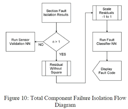
From Figure 10 above it could be noted that the output from the sectional fault isolation was monitored to see if more than one section had a high probability of being faulty. This was indicated by the n > 1 and if this condition is true then the residuals from the sectional isolation are redone but not squared, thus providing negative values as well. These values are then scaled between -1 to 1 using a tan-sig function and ran through a neural network, which then outputs a fault code which is coupled to a specific failure.

 

9. CONCLUSION

The research done proved that a simple feedforward neural network trained with a gradient descent training algorithm can be used to model a complex closed loop control system. The model could be trained to function as a dedicated neural observer to detect and isolate components or sensors causing oscillatory faults. In order to detect sensor faults using a neural observer the neural network's input-output configuration needed to change; hence a bank of different neural networks was needed to detect sensor and component faults, where the number of neural networks was equal to the number of sensors being monitored.

The neural observer's accuracy was dependent on the amount of training data available, where it was beneficial to include all normal operational data, which would enable the observer to accurately estimate outputs from all different conditions of the plant. This was noted in this application where for oscillatory faults the neural observer was only trained to estimate outputs from the locomotive's power notch 1 and 2, due to the fact that excessive oscillation could be detected in the locomotive's power notch 1. When the FDI system's abilities to isolate total component failures were tested, it was found that it could not sufficiently isolate the faults with the design for the detection and isolation of oscillatory faults. Analysis of the input data to the different neural observers indicated that it was due to the control system increasing its reference input to try to compensate for the no output condition of the failing component. It was also noted that the reference input was increased to power notch 8 of the locomotive's power notches, but with the observer trained with data gathered from the locomotive's power notch 1 to 2 it could not sufficiently estimate outputs from the locomotive's power notch 8's reference input; thus it could not isolate the fault sufficiently. The detection of a total component failure was not the primary concern in this dissertation as the locomotive's human machine interfacing module (HMI) could detect total component failures, but due to the fact that .rec files could be loaded into the GUI application the paper included an extension which satisfactorily isolated total component faults.

The residual evaluation technique was of utmost importance and it was found that the use of a normal fault count method which incremented if a residual exceeded a threshold was insufficient due to the fact that all signal feedbacks oscillate in the system if a sensor or component starts to oscillate. An alternative approach was used, which incorporated the use of a tan-sig and percentage above the threshold function. This function sufficiently isolated the faulty components and sensors in the case of oscillatory faults.

It was also noted that the oscillatory conditions were increased whenever a negative was removed from a sensing unit and even then the FDI system sufficiently isolated the faulty component, but with the decision margins being closer to each other than for normal oscillatory faults.

In conclusion to the research done, it could be noted that the developed FDI system isolated oscillatory faults with high confidence and produced a 100% accuracy for the detection and isolation of the sensor or component causing the oscillation. The use of a neural observer model indicated that some knowledge of the system or plants architecture with regard to input-output configuration was necessary to develop an optimum FDI system. This knowledge of the system would enable the neural network to be trained on true cause and effect data, making training easier and errors smaller. The overall aim of the dissertation, which was to develop a user friendly software based FDI system to isolate faults which cause oscillations, was successfully implemented.

9.1 Future Research

More research is required in the use of the probability data to perform preventative maintenance. This would incorporate the use of data analysis of a normal performing locomotive's excitation control system during its service every 45 days. The analysis will entail the recording of the probability results from testing the locomotive gathered from the developed FDI system, as indicated in Figure 7, and using this data to predict a possible remaining life cycle for the sensing components. Research into the use of different threshold limits to detect small oscillations due to interference or dirty components will also be done in an effort to increase the stability of the excitation system.

The ultimate result would be to design a system which could perform FDI onboard through the use of a network interfacing protocol. Fault isolation in terms of a redundant system which could isolate a faulty sensor reading and still have the locomotive operate normally to its service depot, would be the end result.

 

10. REFERENCES

[1] R. Isermann, Fault Diagnosis Applications, Darmstadt: Springer, 2010.         [ Links ]

[2] M. J. Bagajewicz and D. J. Chmielewski, Smart Process Plants Software and Hardware Solutions for Accurate Data and Profitable Operations, New York, Chicago, San Francisco, Lisbon, London, Madrid, Mexico City, Milan, New Delhi, San Juan, Seoul, Singapore, Sydney, Toronto: The McGraw-Hill Companies, Inc, 2010.         [ Links ]

[3] R. Isermann, "Model-based fault detection and diagnosis - status and applications," Elsevier Ltd, Darmstadt, Germany, 2005.

[4] N. P. Srivastava, R. K. Srivastava and P. K. Vashishtha, "Fault Detection and Isolation (FDI) Via Neural Networks," Journal of Engineering Research and Applications, vol. IV, no. 1, pp. 81-86, 2014.         [ Links ]

[5] K. Patan, Artificial Neural Networks for the Modeling and Fault Diagnosis of Technical Processes, Poland: Springer, 2008.         [ Links ]

[6] S. Singh and T. V. R. Murthy, "Neural Network based Sensor Fault Detection for Flight Control Systems," International Journal of Computer Applications, vol. 59, no. 13, pp. 1-8, 2012.         [ Links ]

[7] L. Mhamdi, H. Dhouibi, N. Liouane and Z. Simeu-Abazi, "Detection and localization method of Single and Simultaneous faults," International Journal of Engineering and Science, vol. 1, no. 7, pp. 25-35, 2012.         [ Links ]

[8] Y. Kourd, D. Lefenvre and N. Guersi, "Fault Diagnosis Based on Neural Networks and Decision Trees: Application to DAMADICS," International Journal of Innovative Computing, Information and Control, vol. 9, no. 8, pp. 3185-3196, 2013.         [ Links ]

[9] M. Addel-Geliel, S. Zakzouk and M. El Sengaby, "Application of Model based Fault Detection for an Industrial Boiler," in Mediterranean Conference on Control & Automation (MED), Barcelona, Spain, 2012.

[10] R. Yusof, F. S. Ismail, R. Zafira and A. Rahman, "Model-based Fault Detection and Diagnosis Optimization for Process Control Rig," IEEE, pp. 16, 2013.

[11] P. F. Odgaard, B. Lin and S. B. Jorgensen, "Observer and Data-Driven-Model-Based Fault Detection in Power Plant Coal Mills," IEEE TRANSACTIONS ON ENERGY CONVERSION, vol. 23, no. 2, pp. 659-668, 2008.         [ Links ]

[12] J. Chen, "Robust Residual Generation for Model-Based Fault Diagnosis of Dynamic Systems," University of York, 1995.

[13] I. Samy and G. Da-Wei, Fault Detection and Flight Data Measurement: Demonstrated on Unmanned Air Vehicles using Neural Networks, Berlin: Springer, 2012.         [ Links ]

[14] J. Korbicz, J. M. Koscielny, Z. Kowalczuk and W. Cholewa, Fault Diagnosis: Models, Artificial Intelligence, Applications, Berlin: Springer Science & Business Media, 2012.         [ Links ]

[15] B. Koppen-Seliger and P. M. Frank, "Fault Detection and Isolation in Technical Processes with Neural Networks," in Conference on Decision & Control, New Orleans, LA, 1995.

[16] E. Alcorta Garcia, M. Schubert and P. M. Frank, "Fault Isolation In a Winding-Machine Using RCE Networks," in European Control Conference, Karlsruhe, Germany, 1999.

[17] A. P. Engelbrecht, Computational Intelligence: An Introduction Second Edition, Chichester, England: John Wiley and Sons Ltd, 2007.         [ Links ]

[18] J. Gao, Digital Analysis of Remotely Sensed Imagery, New York, Chicago, San Francisco, Lisbon, London, Madrid, Mexico City, Milan, New Delhi, San Juan, Seoul, Singapore, Sydney, Toronto: The McGraw-Hill Companies, Inc, 2009.         [ Links ]

[19] J. Guo, Y. Liu, X. Xu and Q. Chen, "Integrated distributed bond graph modeling and neural network for fault diagnosis system of hydro turbine governors," Kybernetes, vol. 39, no. 6, pp. 925-934, 2010.         [ Links ]

[20] H. Taplak, Í. Uzmay and §. Yildinm, "An artificial neural network application to fault detection of a rotor bearing system," Industrial Lubrication and Tribology, vol. 58, no. 1, pp. 32 - 44, 2006.         [ Links ]

[21] S. Mousavi and K. Khorasani, "Fault detection of reaction wheels in attitude control subsystem of formation flying satellites: A dynamic neural network-based approach," International Journal of Intelligent Unmanned Systems, vol. 2, no. 1, pp. 2 -26, 2014.         [ Links ]

[22] N. Saravanan, A. Duyar, T. Guo and W. Merrill, "Modeling of the Space Shuttle Main Engine Using Feed-forward Neural Networks," in American Control Conference, San Francisco, California, 1993.

[23] M. R. Napolitano, G. Silvestri, D. A. Windon II, J. L. Casanova and M. Innocenti, "Sensor Validation Using Hardware-Based On-Line Learning Neural Networks," IEEE TRANSACTIONS ON AEROSPACE AND ELECTRONIC SYSTEMS, vol. 34, no. 2, pp. 456-468, 1998.         [ Links ]

[24] K. Funahashi, "On the approximate realization of continuous mappings by neural networks," Neural Networks, vol. 2, no. 3, pp. 183-192, 1989.         [ Links ]

[25] A. Engelbrecht, Computational Intelligence, Chichester: John Wiley & Sons, Ltd, 2002.         [ Links ]