


Services on Demand
Article
 English (pdf)
 Article in xml format
 Article references
Indicators

Related links
-
 Cited by Google
 -
 Similars in Google
Share

 Permalink
Water SA
On-line version ISSN 1816-7950
Print version ISSN 0378-4738
Water SA vol.50 n.1 Pretoria Jan. 2024
http://dx.doi.org/10.17159/wsa/2024.v50.i1.4067
RESEARCH PAPER
Alternative streamflow-based approach to estimate catchment response time in medium to large catchments: case study in Primary Drainage Region X, South Africa
OJ GerickeI; JPJ PietersenI; JC SmithersII; JA Du PlessisIII
IDepartment of Civil Engineering, Central University of Technology, Free State, Bloemfontein, South Africa
IICentre for Water Resources Research and School of Engineering, University ofKwaZulu-Natal, Pietermaritzburg, KwaZulu-Natal, South Africa
IIIDepartment of Civil Engineering, Stellenbosch University, P/Bag X1, Matieland 7602, South Africa
ABSTRACT
Event-based estimates of the design flood in ungauged catchments are normally based on a single catchment response time parameter expressed as either the time of concentration (Tc), lag time (TL) and/or time to peak (Γρ). In small, gauged catchments, a simplified convolution process between a single observed hyetograph and hydrograph is generally used to estimate these time parameters. In medium to large heterogeneous, gauged catchments, such a simplification is neither practical nor applicable, given that the variable antecedent soil noisture status resulting from previous rainfall events and spatially non-uniform rainfall hyetographs can result in multi-peaked hydrographs. In ungauged catchments, time parameters are estimated using eithei empirical or hydraulic methods. In South Africa (SA), unfortunately, the majority of the empirical methods recommended for general use were developed and verified in catchments < 0.45 km2 without using any local data. This paper presents the further development and verification of the streamflow-based approach developed by Gericke (2016) to estimate observed Tp values and to derive a regional empirical Tp equation in Primary Drainage Region X, SA. A semi-automated hydrograph analysis tool was developed to extract and analyse complete hydrographs for time parameter estimation using primary streamflow data from 51 flow-gauging sites. The observed TP values were estimated using three methods: (i) duration of total net rise of a multi-peaked hydrograph, (ii) triangular-shaped direct runoff hydrograph approximations, and (iii) linear catchment response functions.The combined use of these methods incorporated the high variability of event-based time parameters, and Method (iii), in conjunction with an ensemble-event approach sampled from the time parameter distributions, should replace the event-based approaches to enable the improved calibration of empirical time parameter equations. The conceptual approach used to derive the regional empirical Tp equation should also be adopted when regional equations need to be derived at a national scale in SA.
Keywords: catchment response time, design flood estimation, time of concentration, time parameter, streamflow
INTRODUCTION
Deterministic event-based design flood estimation (DFE) methods are commonly used by practitioners in ungauged catchments (Van Vuuren et al., 2012). In the application of these deterministic event-based DFE methods (e.g., rational, standard design flood, lag-routed hydrograph, etc.), it is widely assumed that the peak discharge from a catchment occurs when the duration of rainfall over a catchment equals the time of concentration (T'c), i.e., when the entire catchment is contributing to runoff at the outlet. In applying other deterministic event-based DFE methods, e.g., synthetic unit hydrograph method, a trial-and-error approach is used to establish the storm duration which will result in the highest peak discharge. Thus, irrespective of whether the storm duration is Tc-based or user-defined, the estimation of the catchment response time is necessary to select the critical duration of design rainfall to estimate the peak discharge using deterministic event-based DFE methods. Apart from Tc, catchment response time could also be expressed using other time parameters, e.g., lag time (TL) and/or time to peak (Tp). These time parameters are not only regarded as a fundamental input to deterministic event-based DFE methods, but any errors associated with these time parameter estimates will directly impact on peak discharge and volume estimates (McCuen, 2009; Gericke and Smithers, 2014).
In considering observed rainfall hyetographs and streamflow hydrographs in gauged catchments, time parameters (e.g., Tc, TL and/or Tp) can be defined by considering the time interval difference between two interrelated observed time variables, each obtained from a hyetograph (e.g., maximum rainfall intensity, centroid of effective rainfall, and/or the end time of a rainfall event) and/or a hydrograph (e.g., peak discharge, centroid of direct runoff, and/or the inflection point on the recession limb) (McCuen, 2009). In small, gauged catchments, a simplified convolution process is generally used to estimate time parameters. However, this simplification is neither practical nor applicable in medium to large heterogeneous, gauged catchments (Gericke and Smithers, 2014; 2017). Apart from the difficulty in applying a similar convolution process in larger catchments to establish the temporal relationship between a catchment hyetograph (derived from numerous rainfall stations) and the resulting outflow hydrograph, a uniform response to rainfall is assumed. Hence, the variable antecedent soil moisture status resulting from previous rainfall events and spatially non-uniform rainfall hyetographs, which can result in multi-peaked hydrographs, are ignored (Gericke and Smithers, 2017). The use of point rainfall data to estimate catchment hyetographs also has several associated problems, e.g., lack of data at sub-daily timescales, poor synchronisation of time between different point rainfall and/or streamflow data sets, and the difficulties experienced when measuring time parameters directly from digitised autographic records (Schmidt and Schulze, 1984). The afore-mentioned limitations associated with point rainfall data are further aggravated by the decline of the South African rainfall monitoring network over recent years. The number of operational South African Weather Service (SAWS) rainfall stations has reduced from more than 2 000 in the 1970s to the current situation where the network is no better than it was as far back as 1920, with currently less than a 1 000 rainfall stations operational in a specific year (Pitman, 2011). Internationally the number of operational rainfall stations is also declining (Lorenz and Kunstmann, 2012). In contrast to rainfall data, streamflow data are generally less readily available internationally but the quantity and quality thereof enable the direct estimation of catchment response times at medium to large catchment scales, while there are approximately 708 flow-gauging sites in South Africa (SA) having more than 20 years of records available (Smithers et al.,2014).
The analyses of hyetograph-hydrograph relationships to obtain time parameters are often performed manually, especially when rainfall-based time variables are required. As a result, such analyses are generally tedious, inconsistent, and subjective. Apart from the automated hyetograph-hydrograph analysis tool recently developed by Allnutt et al. (2020), most of the currently available hydrograph analysis tools (e.g., Arnold et al., 1995; Chapman, 1999; Lim et al., 2005) do not include both rainfall hyetograph and streamflow hydrograph characteristics primarily aimed at the estimation of time parameters. In other words, these automated tools were not primarily developed to identify and define time variables for the subsequent estimation of time parameters, but they rather focus on the estimation of general hydrograph characteristics, direct runoff, baseflow separation, and recession analyses.
In ungauged catchments, catchment response time parameters are estimated using either empirical or hydraulic methods, although analytical or semi-analytical methods are also available (McCuen et al., 1984; McCuen, 2009). Empirical methods are the most frequently used and represent approximately 95% of all the methods developed internationally (Gericke and Smithers, 2014). However, the majority of these empirical methods are applicable to and calibrated for small catchment areas (A), except for A < 1 280 km2 (Thomas et al, 2000), A < 5 000 km2 (Pullen, 1969; Mimikou, 1984; Watt and Chow, 1985; Sabol, 2008), and 20 km2 < A < 35 000 km2 (Gericke and Smithers, 2016).
In SA, unfortunately, none of the empirical Tc estimation methods recommended for general use, e.g., Kerby (1959) and United States Bureau of Reclamation (USBR, 1973) equations, were developed and verified using local data, neither are they applicable to large catchments given that the calibration catchment areas were limited to 0.45 km2 (McCuen et al., 1984). Locally the empirical TL estimation methods are limited to the United States Department of Agriculture Soil Conservation Service (USDA SCS, 1985), SCS-SA (Schmidt and Schulze, 1984), and the Hydrological Research Unit (HRU; Pullen, 1969) equations. The SCS methodologies are limited to small catchments (A < 30 km2), while the HRU methodology typically applies to A < 5 000 km2 (Gericke and Smithers, 2014). Consequently, practitioners commonly apply the Tc and TL methods outside their bounds, both in terms of areal extent and their original developmental regions, without using any local correction factors. As a result, and in line with the research priorities identified by the National Flood Studies Programme (NFSP; Smithers et al., 2014), Gericke (2016) developed a new approach to estimate observed Tp values using only observed streamflow data to calibrate and verify empirical Tp equations in a pilot-scale study in four climatologically different regions of SA. Given that both Gericke and Smithers (2017) and Allnutt et al. (2020) confirmed that TC~TL~ Tp in medium to large catchments, the versatility of the streamflow-based Tp equations to estimate Tc and/or TL is acknowledged.
In considering the status quo in South African flood hydrology related to catchment response time parameters, the aim of this paper is to further develop and verify the streamflow-based approach of Gericke (2016) to estimate observed time to peak (Tpχ) values and to derive a regional empirical Tpy equation in Primary Drainage Region X, SA. The specific objectives are to: (i) develop a semi-automated hydrograph analysis tool (HAT) to extract and analyse complete hydrographs for time parameter estimation and based on primary streamflow data from 51 flow-gauging sites, (ii) estimate the observed Tpx values using 3 methods, e.g., duration of total net rise of a multi-peaked hydrograph, triangular-shaped direct runoff hydrograph approximations, and linear catchment response functions, (iii) derive a regional empirical Tpy equation, and (iv) compare the performance of the derived Tpy equation against existing Tpy equation(s) to highlight the limitations of empirical equations when applied beyond the boundaries of their original developmental regions.
The scope of the study is limited to Primary Drainage Region X, given that the 51 flow-gauging stations generally have better and more complete data sets for which the Department of Water and Sanitation (DWS) has done some stage-discharge extensions. In addition, this paper reports the development of a semi-automated HAT, which will also serve as a future benchmark to inform and support the envisaged development, testing, and verification of a comprehensive (fully automated) hydrograph extraction utility. A summary of the study area is contained in the next section, followed by a description of the methodologies adopted and the results achieved. This is followed by the discussion and conclusions.
STUDY AREA
South Africa, which is located on the southernmost tip of Africa, is demarcated into 22 primary drainage regions, i.e., A to X (Midgley et al., 1994), which are further delineated into 148 secondary drainage regions, i.e., A1, A2, to X4. As shown in Fig. 1, Primary Drainage Region X covers 31 193 km2; 70% extends across the Mpumalanga Province of SA, while the remainder extends into Eswatini (former Swaziland).
Primary Drainage Region X is further delineated into 4 secondary drainage regions, i.e., X1 (11 227 km2), X2 (10 447 km2), X3 (6 322 km2), and X4 (3 197 km2). The 51 gauged catchments under consideration have catchment areas ranging from 6 km2 to 21 583 km2. The catchment topography is moderately steep with elevations varying from 112 m to 2 255 m above mean sea level and with average catchment slopes between 3.5% and 36.1% (USGS, 2016). The mean annual precipitation (MAP) ranges from 521 mm to 1 325 mm (Lynch, 2004) and the summer rainfall is regarded as highly variable. The flow-gauging stations in each catchment are classified by DWS as either primary (P), secondary (S), or tertiary (T) gauging sites based on the: (i) status (open/ closed), (ii) location and importance in the overall monitoring network, (iii) data availability, quality, and record length, (iv) type of calibration (standard/extended for above-structure-limit conditions), (v) site survey information available (yes/no), and (vi) flood frequency analyses conducted (yes/no).
METHODOLOGY AND RESULTS
This section contains the methodology adopted to achieve all the specific objectives and the associated results.
Development of a semi-automated hydrograph analysis tool
The IIAT was developed in the Microsoft Excel and/or Visual Basic for Applications (VBA) environment and includes semi-automalcd routines to enable the identification, extraction, and analyses of complete hydrographs for the purpose of time parameter estimation, as detailed in the subsequent sections. The approximation of Tc ~ Tp as proposed by Gericke (2016) forms the basis of the IIAT and is based on the definition that the volume of effective rainfall equals the volume of direct runoff when a hydrograph is separated into direct runoff and baseflow. As shown in Fig. 2, the separation point on the hydrograph is regarded as the start of direct runoff (QDxi), which coincides with the onset of effective rainfall (Pexi). Hence, the extensive convolution process normally required to estimate time parameters is eliminated, given that the time parameters are estimated directly from the observed streamflow data without the need for rainfall data.

Typically, a complete hydrograph extracted using the HAT will include: (i) start/end date/time of flow event, (ii) observed water level (m), (iii) observed discharge (m3-s') and total volume of runoff (Qtxi, m3), (iv) direct runoff discharge (m3-s-1) and total volume of direct runoff (QDxi, m3), (v) baseflow discharge (m3-s1) and total volume of baseflow (QBxi, m3), and (vi) the cumulative volume of direct runoff under the hydrograph rising limb (QDRi, m3).
Extraction and analysis of flood hydrographs to estimate time parameters
The procedural steps followed in Region X, with the aid of functionalities available in the HAT, include the (Gericke et al., 2023):
(a) Evaluation, preparation, and extraction of primary streamflow data for the period up to 2020/21 from the DWS streamflow database.
(b) Identification and extraction of the annual maximum series (AMS) events, i.e., the annual flood peaks at each flow-gauging station within a hydrological year. For example, a continuous record length of 50 years contains 50 AMS events.
(c) Assessment of the accuracy and relevance of the discharge rating tables (DTs) on the DWS website. In general, all the DTs in the study area were already quality controlled and extended (as required) by DWS (Flood Studies). However, in the absence of an extended DT (if required), the AMS data set was extended using a 3rd order polynomial relationship up to 20%. As recommended by Gericke and Smithers (2017), the verification of the extension to +20% considered both the hydrograph shape, especially the peakedness as a result of a steep rising limb in relation to the hydrograph base length, and the relationship between individual peak discharge (QPxi) and direct runoff volume (QD„) pair values. Typically, in such an event, the additional volume of direct runoff (QDE) due to the extrapolation is limited to 5%, i.e., QDE <. 0.05 Qdxi.
(d) Implementation of user-defined truncation level criteria (Qtr) associated with the record length (N) to extract complete hydrographs. The following truncation level criteria were implemented to ensure that the frequently occurring and lower AMS values, which could potentially result in underestimated time parameters, are excluded:
(i) N < 20 years, use the lowest/minimum AMS value,
(ii) 20 < N< 60 years, use the 25th-percentile AMS value, and
(iii) N > 60 years, use the median AMS value. For example, the median AMS value typically has a return period (T) = 2-ycar or an annual cxceedancc probability (AFP) - 50%. Hence, all complete hydrographs with a peak discharge > selected AMS value, i.e., partial duration series (PDS) values above a certain discharge threshold, were extracted.
(e) Identification and extraction of complete hydrographs (cf. Fig. 2) associated with each AMS event and applicable truncation level criteria. A total of 4 454 complete hydrographs were extracted and analysed. The recordlengths under consideration varied between 13 and 112 years, with an overall average record length of 49 years. The QTR criteria were dominated by the minimum AMS (5 catchments) and 25-percentile AMS (29 catchments) values in 67% of all the catchments under consideration. Therefore, at least 75% of all the AMS events were included in the analyses at a catchment level, while it could be argued that 50% or more of the AMS events were discarded in the 17 catchments (33%) remaining where the median AMS criteria were applied. Given that record length is used as the guide for the QTR criteria, the process followed is regarded as consistent, both in terms of the process itself and the results obtained. Subsequently, it is evident that not all the AMS values need to be included in time parameter analyses. As a result, only 2 284 hydrographs were considered in the final analyses.
(f) Separation of complete hydrographs (cf. Fig. 2) into direct runoff and baseflow. The recursive digital filtering method (Eq. 1) as initially proposed by Lyne and Hollick (1979), further developed by Nathan and McMahon (1990), and implemented by Smakhtin and Watkins (1997) in a national scale study in SA, was used to separate the direct runoff and baseflow. Equation 1 is also the preferred baseflow separation method used by DWS and included as the default digital filter algorithm in the Hydrological Timeseries Data Management System (Hydstra) which is used to manage and maintain the whole DWS meteorological and hydrological database. Given that daily/sub-daily time-step data are more appropriate to time parameter estimation and the need for consistency and reproducibility, Eq. 1 with default α-parameter values ranging between 0.995 and 0.997 (Smakhtin and Watkins, 1997), and a fixed β-parameter value of 0.5 (Hughes et al., 2003), was used in all the catchments under consideration.

where: QDxi is the filtered direct runoff (m3 -s-1) at time step i, which is subject to QDx > 0 for time i, α, β are the filter parameters, and QTxi is the total streamflow (m3-s-1; direct runoff plus baseflow) at time i.
(g) Estimation of the time parameter values associated with individual hydrograph/flood events using two different approaches: (i) net rise (duration) of a multi-peaked hydrograph (Eq. 2), and (ii) triangular-shaped direct runoff hydrograph approximation (Eq. 3) and associated variable hydrograph shape parameters (Eqs 3a-c) as shown in Fig. 3.

where: TBxi is the triangular hydrograph base length (h) for individual hydrograph/flood events, t] is the duration of the total net rise (excluding the in-between recession limbs) of a multiple-peaked hydrograph (h), Tpxi. is the net rise (duration) or triangular approximated time to peak (h) for individual hydrographs/flood events, TRcxi is the recession time (h) for individual flood events, QDxi is the volume of direct runoff (m3) for individual hydrographs, QDRi is the volume of direct runoff (m3) under the rising limb for individual hydrographs, QPxi. is the observed peak discharge (m3-s-1) for individual hydrographs, K is the hydrograph shape parameter, N is the sample size, and x is a variable time parameter proportionality ratio, with x = 1, either Tpxi or Tpx and/or TCxi or TCx could be estimated, while TLxi or TLx could be estimated by assuming that TL = 0.6TC, which is the time from the centroid of effective rainfall to the time of peak discharge.
Equation 2 was adopted from Du Plessis (1984). Given that the complete hydrographs extracted are based on the user-defined truncation level criteria, hydrographs containing multiple peaks as shown in Fig. 2 could be possible. Hence, in applying Eq. 2, hydrographs are regarded as separate events when the start of a successive rising limb is characterised by the total discharge = baseflow discharge. If the total discharge > baseflow discharge, then the net rise calculation continues from the trough after the previous peak. Therefore, Eq. 2 is regarded as the best estimate of the observed TPxi values as extracted directly from the observed hydrographs.
A scatter plot of the Tρ„ values computed using Eqs 2 and 3 for all the catchments under consideration is shown in Fig. 4. In comparing Eqs 2 and 3 at a catchment level, the r2 value of 0.84 (based on the 2 284 flood hydrographs) not only confirms the relatively high degree of association, but also the usefulness of Eq. 3. Taking into consideration the influence that catchment area has on response times, the degree of association between these individual TPxi values could decrease with an increase in catchment area. In the case of deterministic event-based DFE, the ultimate goal is to estimate the average catchment TPx by considering the sample-mean of the individual responses based on Eqs 2 and 3, respectively. However, these individual responses can also be used to fit distributions for future ensemble-event approaches (Nathan and Ling, 2016).

In Fig. 5, a frequency distribution histogram of the QDRi values expressed as a percentage of the total direct runoff volume (QDxi) is shown. Taking into consideration that 2 284 (51.3%) of the individual flood hydrographs extracted were included in the final analyses, a few flood events could be characterised by either low (0.4%) or high (92.8%) QDRi values. However, approximately 35% of the QDRi values are within the 20 ~ 40% range. Only 15% of the QDRi values are within the 30 ~ 40 % range; highlighting some relevance of the conceptual curvilinear unit hydrograph theory (USDA NRCS, 2010) which assigns 37.5% of the direct runoff volume to the hydrograph rising limb.
Thus, by using the above approach, as detailed in Step (g), both multi-peaked hydrographs (Eq. 2) and triangular-shaped direct runoff hydrograph approximations (Eq. 3) are included. Ultimately, Eq. 3, which reflects the actual percentage of direct runoff under the rising limb of each individual hydrograph, can also be used in future to expand the unit hydrograph theory to larger catchments. In other words, the variable hydrograph shape parameter (Eq. 3a), which reflects the actual percentage of direct runoff under the rising limb of each individual hydrograph, can be used instead of the fixed volume of 37.5% normally associated with the conceptual curvilinear unit hydrograph theory.
(h) Estimation of the 'average' catchment response time (TPx) of all the flood events considered in each catchment by using a linear catchment response function (Eq. 4), i.e., ihe relationship between individual paired observed peak discharge (QPxi) and direct runoff volume (QDxi) values.
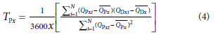
where; TPx is the 'average' catchment time to peak (h) based on a linear catchment response function, QDxi is the volume of direct runoff (m3) for individual hydrographs, QDx is the mean of QDxi. (m3), Qpxi is the observed peak discharge (m s -1) for individual hydrographs, QPx is the mean of QPxi (m3-s-1), N is the sample size, and χ is a variable time parameter proportionality ratio as defined before.
A scatter plot of the average TPxi values computed using both Eqs 2 and 3 in comparison to the catchment TPx values (Eq. 4) for all the catchments under consideration is shown in Fig. 6.
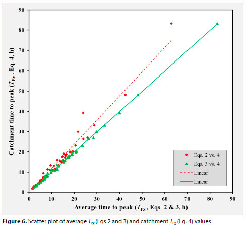
In Fig. 6, a high degree of association is evident, i.e., r2 = 0.986 (Eqs 2 vs. 4) and r2 = 0.999 (Eqs 3 vs. 4). At a catchment level, the averages of Eqs 2 and/or 3 were also comparable to those estimates based on Eq. 4, with average relative differences limited to 13.6% and r2 values ranging from 0.97 to 0.99. Hence, the catchment response times based on an assumed linear catchment response function (Eq. 4) provide results comparable to the sample-mean of all the individual response times as estimated using Eqs 2 and/or 3. The combined use of Eqs 2 and 3 not only incorporates the high variability of event-based time parameters, but the catchment TPx values (Eq. 4) arc also well within the range of other uncertainties inherent to all DFE procedures. Given that Eq. 4 provides a single, average catchment TPx value as required for deterministic event-based DFE, the use thereof in design hydrology and for the calibration of empirical time parameter equations, is recommended.
Calibration, verification, and comparison of regional empirical time parameter equations
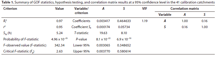
Stepwise multiple regression analyses were performed on the Tpx values (Eq. 4) and geomorphological catchment characteristics (e.g., area A, perimeter P, centroid distance Lc, hydraulic length Lh, average catchment slope S, average main watercourse slope SCH, drainage density DD, and MAP) as included in Table A1 (Appendix) to establish the calibrated TPy relationship (Eq. 5). Both untransformed and log-transformed data sets applicable to the above predictor variables were considered. In some of the 41 calibration catchments, the transformed predictor variables performed less satisfactorily when included as part of the multiple regression analyses, while the log-transformations resulted in negative response times. Subsequently, backward stepwise multiple linear regression analyses with deletion using untransformed data resulted in the best calibrated TPv regression and the following independent and statistically significant predictor variables were retained in Eq. 5 at a 95% confidence level: A and S. Equation 5 was also independently verified in 10 catchments not used during the calibration process.

where: Tpy is the estimated time to peak (h), A is the catchment area (km2), and S is the average catchment slope (%).
The goodness-of-fit (GOF) statistics and correlation matrix applicable to the predictor variables are summarised in Table 1. Typically, the coefficient of multiple-correlation (Ri2) and the standard error of the estimate (SEy) serve as measures of accuracy while the partial f-tests highlight the statistical significance of the individual predictor variables, and the total F-tests represent the degree of correlation between the TPx. values and the predictor variables. In the correlation matrix, the degree of association between the predictor variables is defined using both the coefficient of determination (r2) and the variance inflation factor (VIF). Standardised residuals were also considered to identify possible outliers.
At a 95% confidence level and degrees of freedom = 39, the critical f-statistic (ta) = 2.02. In comparing the f-statistic values of each predictor variable in Table 1 with tx, it is evident that all f-statistic values > tx; hence, confirming the statistical significance of these predictor variables and supporting their inclusion in Eq. 5. The latter results are further supported by all P-values being less than the significance level of 0.05.
It is evident from the correlation matrix that a low correlation exists between the statistically significant predictor variables, with r2 = 0.16, and this is further supported by the VIF =1.19. Typically the lowest VIF value that can be achieved equals one (1), while the range 1 < VIF < 3 is associated with an acceptable to moderate correlation between predictor variables (Mediero and Rjeldsen. 2014). Hence, no collinearity exists between A and S, and they are both regarded as independent and statistically significant predictor variables. The inclusion of a slope predictor (S) is also regarded as essential to ensure that the size (A) predictor provides realistic catchment response times.
Lastly, the SEy, results (= 5.2 hours) in Table 1 must also be clearly understood in the context of the actual travel time associated with the catchment sizes in the study area, as the impact of such an error in the Tpy estimates might be critical in smaller catchments, it would be regarded as less significant in a larger catchment. The rejection of the null hypothesis (F > Fa) in Table 1 also confirmed the significant relationship between TPx and the statistically significant predictor variables as included in Eq. 5.
In considering the standardised residuals computed in both the calibration and verification catchments, it was evident that ± 92% of the total sample have standardised residuals less than ± 2 (ranging between -1.68 and 1.56), except in the case of the calibration catchment, Catchment X2H005 (-2.22), and the verification catchments, Catchments X2H025 (2.04), X2H026 (2.20) and X2H028 (2.39), respectively. However, the three verification catchments have areas ranging from 6 to 25 km2; hence, these catchments are regarded as 'small catchments' and not necessarily 'medium to large catchments', which this study focuses on. According to Chatterjee and Simonoff (2013), it is expected of a reliable regression model to have approximately 95% of the standardised residuals between -2 and +2, while standardised residuals > ± 2 should be investigated as potential outliers. The standardised residuals > ± 2 in the four identified catchments are regarded as 'acceptable', given that TPy is consistent with the regression relationship implied by the other TPx values as included in Fig. 7.

The high degree of association, as depicted in Fig. 7, not only confirmed the good correlation between Tpx and TPv, but also the usefulness of Eq. 5 to estimate the catchment response time in both the calibration and verification catchments. The overall r2 value equals 0.95.
Given the high TPxi variability observed at a catchment level, the lower TPxi values (Eqs 2 and/or 3), which could be associated with rainfall events not covering the whole catchment and centred near the catchment outlet, occur more frequently, and thereby the average value, i.e., the catchment TPx (Eq. 4), could be underestimated. On the other hand, the longer TPxi values have a lower frequency of occurrence and are assumed to be reasonable at medium to large catchment scales as the contribution of the whole catchment to peak discharge seldom occurs as a result of the non-uniform spatial and temporal distribution of rainfall in a catchment. Furthermore, in some catchments (e.g., X2H010, 13-15,26,27, andX2H028), the correlation between the QPxi-QDxi pair values used to derive Eq. 4 is low (r2 ~ 0.1), despite the high agreement (differences < 15%) between Eq. 4 and the averages of Eqs 2 and/or 3 in these catchments. Therefore, it could be argued that the Tpx values (Eq. 4) in the above cases might contribute to less appropriate Tpy estimates (Eq. 5) and need to be further investigated or improved by using an ensemble-event approach sampled from the TPxi distributions.
It is thus evident from the above paragraph that the non-uniform spatial and temporal distribution of rainfall implies that the whole catchment area (A) will seldom contribute to the resulting peak discharge at the catchment outlet. However, A is included in Eq. 5 without being able to consider the spatial and temporal variability. Subsequently, this serves as a further motivation that an ensemble-event approach should be deployed in future to address the uncertainty associated with individual catchment response times and to provide a probabilistic range of acceptable catchment response times at a catchment/regional level which can ultimately be used to improve the calibration of empirical time parameter equations.
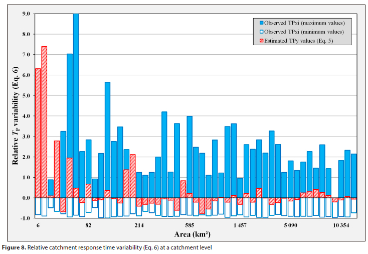
Hence, the high variability of individual-event observed TPxi (Eqs 2 and 3) and estimated Tpv (Eq. 5) values relative to the catchment TPx (Eq. 4) values in each catchment was further investigated using Eq. 6. The relative catchment response time variability or error at a catchment level are shown in Fig. 8.

where: TPVar, is the relative catchment response time variability/ error [over/underestimation (±)], TPx is the observed catchment response time (Eq. 4, h), TPxi is the maximum/minimum individual-event catchment response time (Eqs 2 and/or 3, h), and TPy is the estimated catchment response time (Eq. 5, h).
The high Tpxi variability as depicted in Fig. 8 is not only associated with an increase in catchment area, given that the variability ranges implied by Eq. 6 do not constantly increase with an increasing catchment area. Thus, it could be argued that such higher variabilities could also be associated with an increase in the spatial and temporal distribution and heterogeneity of other geomorphological catchment characteristics and rainfall as the catchment scale increases. Furthermore, the validity of the GOF results listed in Table 1 is also confirmed by and evident from Fig. 8, since the TPy estimates are well within the bounds of the maximum/minimum individual-event observed TPxi variability in each catchment, except in the verification catchments smaller than 25 km2 where the Tpy estimates are associated with standardised residuals > ±2.
In order to compare the performance of the derived Tp, equation (Eq. 5) against existing equation(s), the empirical Tp, equation (Eq. 7) as originally developed by Gericke (2016) was also tested in the 51 catchments. As a result, a scatter plot of the Tpy (Eq. 7) and catchment TPx (Eq. 4) values for both the calibration and verification catchments is shown in Fig. 9 to highlight the limitations when empirical equations are applied beyond their developmental regions.
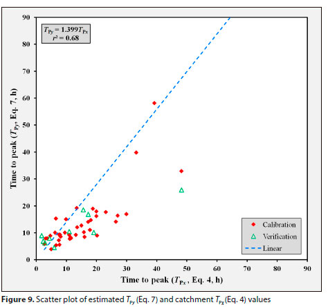

where: Tpy is the estimated time to peak (h), A is the catchment area (km2), Lc is the centroid distance (km), LH is the hydraulic length (km), MAP is the mean annual precipitation (mm), S is the average catchment slope (%), and xl to x5 are calibration coefficients (Gericke, 2016).
The low to moderate degree of association (r < 0.68), as depicted in Fig. 9, highlighted that Eq. 7 in its current format would not be useful to estimate the catchment response time in most of the catchments under consideration, and thereby confirms that any empirical equation should be used with caution when applied beyond the boundaries of its original developmental regions. In addition, many of the standardised residuals exceeded the benchmark standardised residual value of ± 2. Typically, none of the 51 catchments considered in this study formed part of the catchments used to calibrate and verify Eq. 7. Subsequently, Eq. 5 is the preferred empirical equation to estimate TPy, in Primary Drainage Region X.
DISCUSSION AND CONCLUSIONS
The aim of this study was to further develop and verify the streamflow-based approach of Gericke (2016) in Primary Drainage Region X, SA. By achieving the research aim, observed TPx values were estimated in a practical and objective manner without the need for rainfall data to ultimately derive a regional empirical TPy equation. The development of the HAT enabled the consistent extraction and analyses of complete hydrographs for the purpose of time parameter estimation using Eqs 2, 3, and/or 4. Given the high variability and complexities involved when time parameters are estimated, along with the technical problems encountered with observed streamflow data, e.g., exceedance of DTs, multi-peaked hydrographs, etc., a fully-automated version of the HAT is preferred and would typically be required to deploy the proposed methodology at a national scale. Given that the whole DWS meteorological and hydrological database is managed, populated, maintained, and archived using Hydstra, it is recommended that the fully-automated HAT should be based on the current Hydstra tools available. This will not only ensure that the current Hydstra functionalities are optimally utilised, but will also enhance the possibilities of having the HAT built into a web-based version of Hydstra to enable practitioners to run the hydrograph extraction and analyses themselves. As part of the fully-automated HAT to be developed, with specific reference to design hydrology and for the calibration of empirical time parameter equations, the catchment TPx. (Eq. 4) and an ensemble-event approach sampled from the TPxi distributions should be applied in future to replace the current event-based approaches to enable the improved calibration of empirical time parameter equations.
The conceptual approach used to derive the regional empirical TPy equation (Eq. 5) should also be adopted when regional empirical time parameter equations need to be derived at a national scale in SA. However, the application of Eq. 5 should be limited to Primary Drainage Region X, given the known limitations when empirical equations are applied beyond their developmental boundaries. Thus, when attempting to derive any new regional empirical time parameter equation(s) in SA, caution should be practiced by including, as far as possible, only predictor variables which are statistically significant, independent, easy to derive, and commonly available and used in practice. Hence, a balance needs to be achieved between the statistical correctness and user-friendliness of such empirical time parameter equations.
Very often in hydrology, as in this case study, predictor variables might be statistically significant but, due to a high degree of multi-collinearity, the regression coefficient estimates and P-values in the regression model are likely to be unreliable. For example, it is well known in flood hydrology that A, Lc, and LH in combination are useful to describe differences in catchment shape, which subsequently has an impact on the catchment response time. However, these predictor variables are very often associated with a high degree of multi-collinearity, especially Lc and LH. The inclusion of both Lc and LH, subjected to alternative statistical transformations to result in orthogonal variables, should therefore be considered, especially in catchments characterised by heterogeneous upper and lower catchment slope distributions where large differences between S and SCH exist. Typically, the inclusion of Lc ensures that the runoff volumes which reach and concentrate at the catchment centroid much quicker (due to a steeper catchment slope in the upper reaches), in conjunction with the shorter Lc distances to follow to the catchment outlet, result in the required shorter response times. The opposite is also true; hence, the response of a catchment is most likely to be influenced by a combination of geomorphological catchment characteristics and not by a single catchment characteristic, irrespective of whether such characteristics are statistically independent or not. Furthermore, the combined use of A, Lc, and LH is also evident from hydrological literature applicable to the derivation of time parameter equations, e.g., Tc equations (Sabol, 2008), TL equations (Snyder, 1938; Taylor and Schwarz, 1952; Pullen, 1969), and Tp equations (Gericke and Smithers, 2016). It is acknowledged that some of these equations were developed many years ago, but they are still widely used in practice with great success.
In the interim, and in the absence of a fully-automated HAT, it is also recommended that the current methodology be gradually expanded to Primary Drainage Regions A and B, before deploying it at a national scale. Approximately 110 gauged catchments covering the whole of the Gauteng, Mpumalanga, and Limpopo Provinces are situated in these regions. Typically, these three regions do not only form a continuous geographical region, but the largest percentage of SAs population also resides here and is frequently subjected to extreme flooding.
ACKNOWLEDGEMENTS
The study was funded by the Central University of Technology, Free State (CUT) and the Water Research Commission (WRC) through WRC Project No. K5-2924. A number of special acknowledgements deserve specific mention: (i) DWS for providing the observed streamflow data, (ii) Annette Joubert and Gina Gaspar for their assistance in extracting and quality-controlling the DWS streamflow data, (iii) Pieter Rademeyer (DWS) for sharing the geographical information system (GIS) data sets applicable to the study area, (iv) the WRC Reference Group members for their contributions made towards the project, and (v) the anonymous reviewers for their constructive review comments, which have helped to significantly improve the paper.
AUTHOR CONTRIBUTIONS
Jaco Gericke (OJG) conceptualised the study, developed the methodology, and conducted the data analyses. Jaco Pietersen assisted with the data collection and compilation of all the GIS-based data sets and maps. Both Jeff Smithers and Kobus du Plessis acted as principal advisors. OJG compiled the first draft, which was reviewed by all the other authors. OJG implemented all the suggested revisions after review.
ORCIDS
OJ Gericke: https://orcid.org/0000-0003-0371-2516
JPJ Pietersen: https://orcid.org/0000-0001-5254-5684
JC Smithers: https://orcid.org/0000-0003-1598-1748
JA Du Plessis: https://orcid.org/0000-0001-8093-6711
REFERENCES
ALLNUTT CE, GERICKE OJ and PIETERSEN JPJ (2020) Estimation of time parameter proportionality ratios in large catchments: case study of the Modder-Riet River Catchment, South Africa, J. Flood Risk Manage. 13 el2628. https://doi.org/10.llll/jfr3.12628 [ Links ]
ARNOLD JG, ALLEN PM, MUTTIAH R and BERNHARDT G (1995) Automated base flow separation and recession analysis techniques. Ground Water 33 (6) 1010-1018. https://doi.org/10.1111/j.l745-6584.1995.tb00046.x [ Links ]
CHAPMAN T (1999) A comparison of algorithms for streamflow recession and baseflow separation. Hydrol. Process. 13 701-714. https://doi.org/10.1002/(SICI)1099-1085(19990415)13:5<701::AID-HYP774>3.0.CO;2-2 [ Links ]
CHATTERJEE S and SIMONOFF JS (2013) Handbook of Regression Analysis. Volume 5. Wiley Handbooks in Applied Statistics, John Wiley and Sons Incorporated, Hoboken. https://doi.org/10.1002/9781118532843 [ Links ]
DU PLESSIS DB (1984) Documentation of the March-May 1981 floods in the Southeastern Cape. Technical Report No. TR120. Department of Water Affairs and Forestry, Pretoria, RSA. [ Links ]
DWAF (Department of Water Affairs and Forestry, South Africa) (1995) GIS data: drainage regions of South Africa. Department of Water Affairs and Forestry, Pretoria, RSA. [ Links ]
GERICKE OJ (2016) Estimation of catchment response time in medium to large catchments in South Africa. Unpublished PhD (Eng.) thesis. Bioresources Engineering, School of Engineering, College of Agriculture, Engineering and Science, University of KwaZulu-Natal, Pietermaritzburg. [ Links ]
GERICKE OJ and SMITHERS JC (2014) Review of methods used to estimate catchment response time for the purpose of peak discharge estimation. Hydrol. Sciences J. 59 (11) 1935-1971. https://doi.org/10.1080/02626667.2013.866712 [ Links ]
GERICKE OJ and SMITHERS JC (2016) Derivation and verification of empirical catchment response time equations for medium to large catchments in South Africa. Hydrol. Process. 30 (23) 4384-4404. https://doi.org/10.1002/hyp.10922 [ Links ]
GERICKE OJ and SMITHERS JC (2017) Direct estimation of catchment response time parameters in medium to large catchments using observed streamflow data. Hydrol. Process. 31 (5) 1125-1143. https://doi.org/10.1002/hyp.11102 [ Links ]
GERICKE OJ, PIETERSEN JPJ, SMITHERS JC, DU PLESSIS JA, ALLNUTT CE and WILLIAMS VH (2023) Development of a regionalised approach to estimate areal reduction factors and catchment response time parameters for improved design flood estimation in South Africa. WRC Report No. 2924/1/23. Water Research Commission, Pretoria. [ Links ]
HUGHES DA, HANNART P and WATKINS D (2003) Continuous baseflow from time series of daily and monthly streamflow data. Water SA 29 (1) 43-48. https://doi.org/10.4314/wsa.v29il.4945 [ Links ]
KERBY WS (1959) Time of concentration for overland flow. Civ. Eng. 29 (3) 174. [ Links ]
LIM KJ, ENGEL BA, TANG ZA, CHOI J, KIM K, MUTHUKRISHNAN S and TRIPATHY D (2005) Automated web GIS based Hydrograph Analysis Tool (WHAT), J. Am. Water Resour. Assoc. 41 (6) 1407-1416. https://doi.Org/10.llll/j.1752-1688.2005.tb03808.x [ Links ]
LORENZ C and KUNSTMANN H (2012) The hydrological cycle in three state-of-the-art reanalyses: intercomparison and performance analysis, J. Hydrometeorol. 13 1397-1420. https://doi.org/10.1175/JHM-D-11-088.1 [ Links ]
LYNCH SD (2004) Development of a raster database of annual, monthly and daily rainfall for Southern Africa. WRC Report No. 1156/1/04. Water Research Commission, Pretoria. [ Links ]
McCUEN RH, WONG SL and RAWLS WJ (1984) Estimating urban time of concentration, J. Hydraul. Eng. 110 (7) 887-904. [ Links ]
McCUEN RH (2009) Uncertainty analyses of watershed time parameters, J. Hydrol. Eng. 14 (5) 490-498. https://doi.org/10.1061/(ASCE)0733-9429(1984)110:7(887) [ Links ]
MEDIERO L and KJELDSEN TR (2014) Regional flood hydrology in a semi-arid catchment using a GLS regression model, J. Hydrol. 514 (2014) 158-171. https://doi.org/10.1016/j.jhydrol.2014.04.007 [ Links ]
MIDGLEY DC, PITMAN WV and MIDDLETON BJ (1994) Surface water resources of South Africa. WRC Report No. 298/2/94. Water Research Commission, Pretoria. [ Links ]
MIMIKOU M (1984) Regional relationships between basin size and runoff characteristics. Hydrol. Sci. J. 29 (1, 3) 63-73. https://doi.org/10.1061/(ASCE)0733-9429(1984)110:7(887) [ Links ]
NATHAN R and LING F (2016) Book 4: Catchment simulation for design flood estimation, Chapter 3: Types of simulation approaches. In: Ball J, Babister M, Nathan R, Weeks B, Weinmann E, Retallick M, and Testoni I (eds). Australian Rainfall and Runoff. Commonwealth of Australia. [ Links ]
PITMAN WV (2011) Overview of water resource assessment in South Africa: Current state and future challenges. Water SA 37 (5) 659-664. https://doi.org/10.4314/wsa.v37i5.3 [ Links ]
PULLEN RA (1969) Synthetic unitgraphs for South Africa. Report No. 3/69. Hydrological Research Unit, University of the Witwatersrand, Johannesburg. [ Links ]
SABOL GV (2008) Hydrologic basin response parameter estimation guidelines. Dam Safety Report, Tierra Grande International Incorporated, Scottsdale, Colorado. [ Links ]
SCHMIDT EJ and SCHULZE RE (1984) Improved estimation of peak flow rates using modified SCS lag equations. ACRU Report No. 17. Department of Agricultural Engineering, University of Natal, Pietermaritzburg, RSA. [ Links ]
SMAKHTIN VU and WATKINS DA (1997) Low flow estimation in South Africa. WRC Report No. 494/1/97. Water Research Commission, Pretoria. [ Links ]
SMITHERS JC, GöRGENS AHM, GERICKE OJ, JONKER V and ROBERTS P (2014) The initiation of a National Flood Studies Programme for South Africa. South African Committee of Large Dams, Pretoria, RSA. [ Links ]
SNYDER FF (1938) Synthetic unit hydrographs. Trans. Am. Geophys. Union 19 447. https://doi.org/10.1029/TR019i001p00447 [ Links ]
TAYLOR AB and SCHWARZ HE (1952) Unit hydrograph lag and peakflow related to basin characteristics. Trans. Am. Geophys. Union 33 235-246. https://doi.org/10.1029/TR033i002p00235 [ Links ]
THOMAS WO, MONDE MC and DAVIS SR (2000) Estimation of time of concentration for Maryland streams, J. Transport. Res. Board 1720 95-99. https://doi.org/10.3141/1720-ll [ Links ]
USBR (United States Bureau of Reclamation) (1973) Design of Small Dams (2nd edn). Water Resources Technical Publications, United States Bureau of Reclamation, Washington, DC, USA. [ Links ]
USDA NRCS (United States Department of Agriculture Natural Resources Conservation Service) (2010) Time of concentration. Chapter 15 (Section 4, Part 630). In: Woodward DE et al. (eds) National Engineering Handbook. United States Department of Agriculture Natural Resources Conservation Service, Washington, DC, USA. [ Links ]
USDA SCS (United States Department of Agriculture Soil Conservation Service) (1985) Hydrology. In: Kent KM et al. (eds) National Engineering Handbook. United States Department of Agriculture Soil Conservation Service, Washington, DC, USA. [ Links ]
USGS (United States Geological Survey) (2016) EarthExplorer. United States Geological Survey. URL: https://earthexplorer.usgs.gov/ (Accessed 19 September 2016). [ Links ]
VAN VUUREN SJ, VAN DIJK M and COETZEE GL (2012) Status review and requirements of overhauling flood determination methods in South Africa. WRC Report No. K8/994/1. Water Research Commission, Pretoria. [ Links ]
WATT WE and CHOW KCA (1985) A general expression for basin lag time. Can. J. Civ. Eng. 12 294-300. https://doi.org/10.1139/l85-031 [ Links ]
 Correspondence:
OJ Gericke
Email: jgericke@cut.ac.za
Received: 23 March 2023
Accepted: 18 December 2023
APPENDIX


