RESEARCH PAPER

 

Using SPI and SPEI for baseline probabilities and seasonal drought prediction in two agricultural regions of the Western Cape, South Africa

 

 

SN Theron^{I, III}; E Archer^II; CJ Engelbrecht^{II, VI}; S Midgley^{III, V}; S Walker^{I, IV}

^IAgricultural Research Council - Natural Resources and Engineering, 600 Belvedere Street, Arcadia, Pretoria 0083, South Africa
^IIDepartment of Geography, Geo-Informatics and Meteorology, University of Pretoria, Lynnwood Road, Hatfield, Pretoria 0002, South Africa
^IIIDepartment of Horticultural Science, Stellenbosch University, Victoria Road, Stellenbosch Central, Stellenbosch 7600, South Africa
^IVDepartment of Soil, Crop and Climate Sciences, University of the Free State, Bloemfontein 9300, South Africa
^VResearch and Technology Development, Department of Agriculture, Western Cape Government, Elsenburg 7607, South Africa
^VISouth African Weather Service, Eco Park, Centurion 0157, South Africa

Correspondence

 

 

---

ABSTRACT

Drought is one of the most hazardous natural disasters in terms of the number of people directly affected. An important characteristic of drought is the prolonged absence of rainfall relative to the long-term average. The intrinsic persistence of drought conditions continuing from one month to the next can be utilized for drought monitoring and early warning systems. This study sought to better understand drought probabilities and baselines for two agriculturally important rainfall regions in the Western Cape, South Africa - one with a distinct rainfall season and one which receives year-round rainfall. The drought indices, Standardised Precipitation and Evapotranspiration Index (SPEI) and Standardised Precipitation Index (SPI), were assessed to obtain predictive information and establish a set of baseline probabilities for drought. Two sets of synthetic time-series data were used (one where seasonality was retained and one where seasonality was removed), along with observed data of monthly rainfall and minimum and maximum temperature. Based on the inherent persistence characteristics, autocorrelation was used to obtain a probability density function of the future state of the various SPI start and lead times. Optimal persistence was also established. The validity of the methodology was then examined by application to the recent Cape Town drought (2015-2018). Results showed potential for this methodology to be applied in drought early warning systems and decision support tools for the province.

Keywords: drought prediction, drought thresholds, drought persistence, rainfall seasonality, early warning

---

 

 

INTRODUCTION

Drought is a persistent natural occurrence that affects all regions across the globe and cuts across a range of economic and social sectors (such as agriculture, tourism, ecosystems, and health) (Edwards et al., 2019). Moreover, drought is one of the most complex and hazardous natural disasters regarding the number of people directly and indirectly affected (Botai et al., 2017). While an exact definition of drought remains contested, drought is a lack of rainfall relative to what is expected (i.e., 'normal') that, when extended over a season or a longer, results in failure to meet the demands of human activities and the environment (Zargar et al., 2011; Lyon et al., 2012).

The Western Cape Province of South Africa experienced a severe drought between 2015 and 2018 (Otto et al., 2018; Sousa et al., 2018). The threat of Day Zero (the day the taps in the Metropolitan City of Cape Town were projected to run dry) was widely publicised both locally and internationally (Odoulami et al., 2021). The drought also had severe consequences for the province's agricultural regions (Theron et al., 2021). Recent studies have shown that between 1988 and 2018, the Western Cape has experienced recurrent meteorological, hydrological, and agricultural droughts (Theron et al., 2021). Studies by Otto et al. (2018) and Pascale et al. (2020) showed that the 2015-2018 drought was made more likely to occur due to anthropogenic climate change and that this trend is expected to continue. The intensity, frequency and wide-reaching impacts of the 2015-2018 drought, along with the threat of climate change, have heightened interest in drought forecasting, monitoring and early warnings for this region. Furthermore, a study by Theron et al. (2022) showed that farmers in the Western Cape rely on weather forecasts to improve resilience to drought. Their paper identified a need for improved drought forecasting. Thus, this study focused on two agricultural regions in the Western Cape in an attempt to address this need.

Meteorological drought events are characterised by their cumulative and time-integrated nature (Lyon et al., 2012). This results in significant continuation or persistence of drought conditions from one month to the next (Lyon et al., 2012). Drought events usually progress slowly over several months, which increases the importance of, and suitability for, real-time monitoring of drought early warning and prediction (Buurman et al., 2014). Lyon et al. (2012) showed that an improved understanding of drought persistence could support drought prediction by quantifying the likelihood of drought conditions at a future time, given that drought conditions have occurred in the immediate past. Drought indices such as the Standardised Precipitation Index (SPI) and Standardised Precipitation and Evaporation Index (SPEI), among others, are quantitative measures that characterise drought intensity by integrating data from one or more variables such as rainfall into a single numerical value (Zargar et al., 2011). Using this relatively simple methodology, drought indices have evolved into the primary tool for communicating drought intensity globally (Zargar et al., 2011).

Archer et al. (2019) investigated the use of hindcasts from a coupled ocean-atmosphere model of the North American Multi-Model Ensemble System to assess seasonal rainfall predictability over the south-western Cape. The study used ranked probability skill scores to assess the ability of hindcasts to produce probabilistic forecasts for the three seasons - spring, winter, and autumn - at a 1-month lead-time for three equiprobable categories of below-, near- and above-normal seasonal rainfall totals. The method was most accurate for the 3-month winter season rainfall forecasts. Results showed less skill in the season onset during the autumn season, and the lowest skill score was for the cessation during the spring season. Johnston and Wolski (2018) investigated whether a statistically valid predictor for winter rainfall totals could be developed. Their method set out to determine whether, if above-average rainfall had been received up to the end of a particular month (in this case April or May) before the start of the winter rainfall season, there would be a greater chance that by the end of the rainfall season of that year the total rainfall would be above average. The study calculated probabilities for forecasts issued at the end of each month and compared them with the annual total until the end of October. It was found that an above-average wet year will be likely if the cumulative rainfall recorded by the end of April (30% for normal and 65% for above normal) is above mean. Similarly, it was found that a low accumulated rainfall by the end of May (60% for below normal, 35% for normal, and 5% for above normal) can predict with some confidence that the year is going to be dry.

Statistical models have been used to provide operational seasonal forecasts of rainfall over southern Africa since 1992 (Mason, 1998). Lyon et al. (2012) developed a simple, statistical methodology to predict the future state of the SPI, given an initial state, evaluated as a function of the seasonal cycle. This methodology is similar to that of Johnston and Wolski (2018) in that it exploits the persistence of the climatological variable being assessed. The study also set out to determine a set of baseline probabilities for drought monitoring. Lyon et al. (2012) used bootstrap resampling of observed weather data to generate two sets of synthetic datasets of monthly rainfall. The first set included seasonality, while in the second set seasonality was removed. Their results showed that seasonality in the variance of accumulated rainfall could enhance or diminish the persistence characteristics of drought indicators.

Thus, considering seasonal cycles in forecasts can provide a considerable source of drought predictability (Lyon et al., 2012).

This study aimed to test the methodology set out by Lyon et al. (2012) for seasonal drought predictions for the winter rainfall region of the Western Cape (WRRWC). The methodology was tested in two distinct rainfall regions of the province: the winter rainfall region and the year-round rainfall region. The methodology was then applied to the case study of the 2015-2018 drought. Finally, the study also tested both the SPI and SPEI indices to compare the use of temperature (as included in SPEI) on predictive skill.

 

DATA AND METHODOLOGY

The method applied in this study is based on the principle that if an initial drought state has been identified, important predictive information can be derived from the persistence of drought indices (for both SPI and SPEI) (Lyon et al., 2012). The study also tested whether the predictive skill of the persistence of drought indices can be enhanced depending on the start time considered or the season. To exploit the persistence characteristics of drought, the analysis made use of autocorrelation (AC). AC is defined as the correlation of a time series with a lagged version of itself, and it can be used to detect recurrence or periodicity in a dataset (Venkatramanan et al., 2019).

Western Cape rainfall regime

The study was conducted in the Western Cape Province of South Africa (Fig. 1). Figure 1 was adapted from Roffe et al. (2019). The province has a diverse rainfall pattern, including a highly seasonal winter rainfall region, a more even spread of annual rainfall along the Cape south coast, as well as a region with predominantly summer rainfall in the north.

The WRRWC experiences a Mediterranean-type climate with cool, wet winters and warm, dry summers (Botai et al., 2017). Rainfall occurs predominately in the winter months of June, July, and August (Odoulami et al., 2021). The region is affected by an array of large-scale forcing mechanisms, but the position of the westerly storm track over the South Atlantic upstream of the southwest of the region is the dominant factor (Midgley et al., 2005). Cut-off lows (COLs) also contribute to the region's rainfall, particularly in autumn and spring (Favre et al., 2013; Roffe et al., 2021).

In addition, several other large-scale mechanisms may contribute to rainfall in the region. Reason and Rouault (2005) suggested that most dry winters are associated with the positive phase of the Antarctic Oscillation (AAO) or Southern Annular Mode (SAM). The SAM forces a pressure difference between mid-and low latitudes, which indirectly affects the position of the southwesterly winds and influences the number of frontal systems reaching the Western Cape (Odoulami et al., 2021). Philippon et al. (2011) found winter rainfall (May-June-July) to be positively correlated with El Nino 3.4 events - however, their findings feature a strong decadal component that appears to be restricted to recent decades from 1979 (Philippon et al., 2011).

The Cape south coast experiences a temperate oceanic climate with warm summers and mild winters (Van Niekerk and Joubert, 2011; Botai et al., 2017). Rainfall is more evenly distributed throughout the year, and there is no pronounced dry season (Van Niekerk and Joubert, 2011; Botai et al., 2017; Roffe et al., 2019). Most of the Cape south coast is influenced by both mid-latitude and, to a lesser extent, tropical weather systems (Braun et al., 2017). The mid-latitude systems that affect the area are cold fronts, ridging highs and COLs, and the tropical influence is generally from tropical-temperate troughs (Engelbrecht et al., 2015). A statistically significant correlation between the El Nino 3.4 index and monthly rainfall totals has been found in the region (Weldon and Reason, 2014). Most wet years correspond to the mature phase of La Nina years. ENSO also affects rainfall along the Cape south coast by increasing the number of COLs reaching southern South Africa (Weldon and Reason, 2014).

Methodology

Monthly rainfall and daily minimum and maximum temperature data for two Agricultural Research Council stations were used for the analysis, chosen due to their location in agriculturally important regions, as well as their completeness, length of records and representativity of the two rainfall regimes. Monthly data were obtained for the entire record length for each station ending in 2018 from the ARC-Agrometeorology Database (ARC, 2018). The Langgewens station has records going back to 1964, while Outeniqua's records started in 1967. Thus, the datasets produced contain 51 or 55 years of data, respectively. In terms of quality checks, the ARC Agrometeorology Programme maintains an operational national agro-climate network of weather stations and a climate databank, using sensors and methods that adhere to the standards of the World Meteorological Organisation (WMO). Collected weather data goes through an automatic quality control check before being published, which includes a missing data check; a high-low range limits check; a rate of change between successive days' observations check; and a consistency check as well as a manual quality check to identify any problems not caught during the automatic quality check (Henningse, 2021). SPI and SPEI were chosen for this study as they require simple computation and minimal, readily available data inputs. SPI is based on rainfall probability for any time scale, requiring only rainfall as an input parameter. It is calculated by aggregating monthly rainfall over various time scales (3, 6, 12 months)). For example, to calculate SPI 3, the rainfall accumulation from month j-2 to month j is summed and attributed to month j (Guenang and Kamga, 2014). After the rainfall has been aggregated, the resulting value is normalised. SPEI uses the basis of SPI but includes temperature as a factor allowing the index to account for the effects of evapotranspiration on drought development through a basic water balance calculation (Vicente-Serrano et al., 2010; Beguería et al., 2014). The water balance equation is calculated as the difference between rainfall and reference evapotranspiration (Beguería et al., 2014). Next, the climatic water balance is calculated at various time scales (similar to that of SPI), and the resulting values are fitted to a PDF to transform the original values to standardised variates (Vicente-Serrano et al., 2010; Beguería et al., 2014).

Drought indices SPI and SPEI were computed for the entire period in the R-SPEI package. This study investigated accumulation periods of 3, 6, 9 and 12 months. The Outeniqua dataset follows a log-normal distribution (skewness = 2.5 and kurtosis = 16.2), while the Langgewens dataset follows a gamma distribution (skewness = 1.6 and kurtosis = 6.9). Thus, for the calculations of SPI and SPEI for the Outeniqua dataset the data were fitted to a log-normal distribution, while for Langgewens the data were fitted to a gamma distribution. The study made use of the Hargreaves equation (Hargreaves and Samani, 1985) for SPEI.

The first objective was to characterise the rainfall and drought regimes for each region. Observed climate data were used to calculate the percentage contribution of each season to the total annual rainfall. Seasons here were described according to Theron et al. (2021) as summer = December, January, February (DJF); autumn = March, April, May (MAM); winter = June, July, August (JJA); and spring = September, October, November (SON).

In the second part of the study, observed climate data were resampled randomly to produce two synthetic datasets of 100 years for each station. Removing monthly AC in the synthetic datasets allows for quantifying how the design of the drought indices influences drought persistence characteristics, thereby determining a baseline for predictability (Lyon et al., 2012). The first set of synthetic data removed the seasonality of rainfall for both stations. This was achieved by sequencing randomly selected monthly values of observed rainfall and temperature data taken from any month during the observed period. This effectively meant that a value in February could be followed by a randomly selected value for July or any other month. This was done 100 times to create 100 synthetic datasets of 55 (or 51) years without seasonality. The second synthetic dataset retained seasonality but removed any trends in the observed data. This was achieved by randomly sampling data from each month and sequencing by month but not by year. This was also repeated 100 times to create 100 synthetic datasets of 55 (or 51) years.

An important aspect of seasonality is the start time considered. For example, in a highly seasonal rainfall region, the probability of rainfall occurring in subsequent months will depend on whether those months fall within or outside of the rainfall season. Lyon et al. (2012) demonstrate that this principle is also true for drought indices such as SPI and SPEI. They showed that the effect of start times on the AC of SPI was most observable at longer accumulation times such as SPI 12. This study set out to determine which start time will enhance and diminish the persistence characteristics of SPI 12 or SPEI 12 for each station using the 100 synthetic datasets with seasonality retained.

The study also set out to determine the seasonal persistence of drought using the seasons as defined above. Persistence was defined by Lyon et al. (2012) as the situation where AC exceeds 0.6 for several consecutive months. A value of 0.6 was chosen because it suggests that more than one-third of the variance can be accounted for (Lyon et al., 2012). Lyon et al. (2012) further set out a methodology for establishing the optimal persistence of drought characteristics. They indicated that, for indices based on consecutive multi-month rainfall such as SPI and SPEI, the signal is found exclusively in the monthly rainfall values shared with the index at the initial and subsequent state. This is described in more detail by Lyon et al. (2012).

Persistence characteristics can be utilised to determine PDFs for various start and lead times. Thus, given any initial SPI value, the probability of future SPI values can be determined by creating a PDF. Since only the inherent persistence of drought is considered, creating a full PDF provides baseline probabilities (Lyon et al., 2012).

Using the formula (Eq. 1), PDFs were created using a standard deviation based on the AC of the lagged SPI index. The mean was calculated using the climatological mean rainfall for the forecast. This was achieved by concatenating the climatological mean rainfall for each month onto the observed rainfall dataset. Since SPI uses an accumulation of rainfall values over several months, at lag 2 for SPI 12, the SPI value will be calculated based on 11 observed values and 1 climatological mean value. For lag 3 the SPI value will be calculated on 10 observed values and 2 climatological mean values. This will accumulate until lag 12, where all the SPI values will be calculated using the climatological mean values. Importantly, since the predictive skill relies exclusively on the knowledge of the initial condition of SPI or SPEI, the signal will be lost after exceeding the lead times of the accumulation period of the drought index. Nonetheless, useful information may still be contained in the knowledge of the initial condition up to several months in advance, depending on the index and the start time considered (Lyon et al., 2012).

where: σ = standard deviation of the forecast, ρ = autocorrelation, l = lag

For drought concerns, the probability that the index is less than a specific trigger limit can be important. Such thresholds can be derived from a cumulative density function (CDF) which can give the probability of a particular value falling below a given threshold. A CDF for each year in 2015-2018 was produced using observed data and the method for creating the PDF described above for a drought threshold of SPI < -1. This threshold was chosen according to the WMO (2012).

 

RESULTS AND DISCUSSION

Climate in the two regions

Analysis of annual and seasonal climate variables (Table 1) shows that both regions have high interannual rainfall variability. Figure 2 highlights the distinct dry and wet seasons at Langgewens and the year-round rainfall at Outeniqua. At the Langgewens station, winter contributes almost 50% to the total annual rainfall. Summer contributes less than 10%, and the other ~ 45% is spread relatively evenly between autumn (~25%) and spring (~ 20%). In contrast, at Outeniqua, spring contributes the most rainfall with almost 30%, while rainfall in summer, autumn and winter contribute 22-25%.

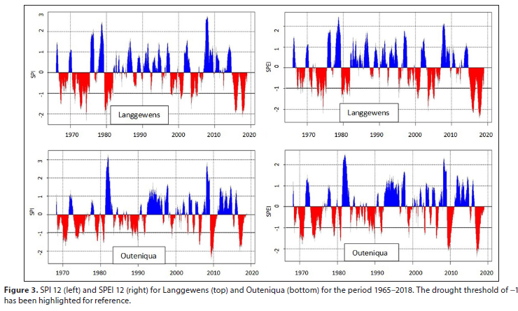
Analysis of drought regimes for the two stations shows slight differences between SPI 12 and SPEI 12, with SPEI 12 showing slightly more severe drought conditions, particularly with regards to the 2015-2018 drought (Fig. 3). Figure 3 shows that Langgewens experiences persistent and recurrent drought conditions, with six mild to severe drought events occurring over the study period. In terms of the 2015-2018 drought, both SPI and SPEI show that the drought began towards the end of 2014, peaked in 2017 and dry conditions extended up to the end of 2018 (end of the dataset). Furthermore, Fig. 3 shows that at Langgewens, drought conditions have only surpassed the -2 index threshold three times (for SPEI) and twice (for SPI 12) during the study period, of which the 20152018 event was the most severe. These results are consistent with that of Botai et al. (2017) and Theron et al. (2021). The Outeniqua station also experiences recurrent and persistent drought, with 11 mild to severe drought events occurring over the study period. Drought conditions surpassed the -2 index threshold once for SPI and twice for SPEI, including the 2015-2018 event. For the Outeniqua station, the 2015-2018 drought began in 2016, also peaking in 2017, and extended up to the end of 2018. Once again, these results are consistent with those of Botai et al. (2017).

Observing persistence in SPI and SPEI indices

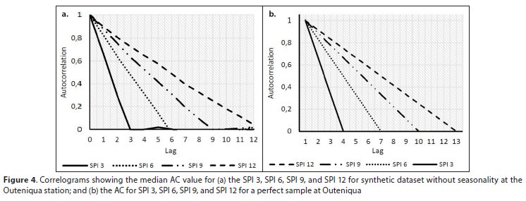
Figure 4a shows the AC of SPI 3, SPI 6, SPI 9 and SPI 12, where seasonality has been purposefully ignored using the 100 synthetical datasets for Outeniqua. As expected, AC drops off linearly with lag for each index, reaching zero when the time lag surpasses the accumulation period of the index (i.e., after 3 months for SPI 3, after 6 months for SPI 6). Since seasonality has been ignored, the ACs shown in Fig. 4 do not depend either on the mean or variance of the rainfall used to calculate the drought index and will thus hold for any region (Lyon et al., 2012). Figure 4b shows an example of the AC of a dataset where the rainfall values are entirely independent. Thus, Fig. 4b can be used to compare the persistence of AC of SPI where rainfall values used to calculate SPI are related in some or other way. The theory behind Fig. 4b is further explained in Lyon et al. (2012). Only SPI is shown since the figure for SPEI will look identical. This is because both indices are based primarily on accumulated rainfall as a percentage of the mean (Lyon et al., 2012).

The effect of seasonality on AC is shown in Fig. 5 for a start time of each month of the year for each station. These results were obtained from the median AC of the 100 synthetic datasets in which seasonality was retained. The information in Fig. 5 allows for the selection of a suitable start time to enhance or diminish the persistence. In addition, Figs 5a and b allow for the comparison of persistence characteristics between SPI and SPEI for the Langgewens station. There is a noticeable difference in the persistence between SPI and SPEI for the Langgewens station, with SPEI showing diminished persistence (indicated by the 'tighter fit' of the lines). This suggests that SPI can better capture persistence in this region and will consequently be more useful for persistence analysis. Outeniqua (Fig. 5c) shows lower SPI persistence characteristics than Langgewens, which was expected since Outeniqua does not have such a pronounced rainfall season (Fig. 2).

While April emerged as the month with the most diminished persistence characteristics, for both SPI and SPEI, there was no clear month that showed the same for enhancement. August, September, October, and November emerged as months where AC is enhanced for several subsequent months. November had the highest AC, but this was only present for the first four lag times, after which AC dropped off relatively steeply. October and September showed lower AC at lag 1 than November, but the AC remained higher for longer and did not drop off as steeply as that for November. August showed lower AC than the other three indices at lag 1 to lag 4 but then remained higher for longer, with AC > 0.5 up to lag 9. In summary, choosing November as a start month will give an enhanced prediction of the SPI conditions in subsequent months (or short lead times) but will quickly lose the skill at longer lead times. August may retain some skill to predict SPI conditions at longer lead times than November, but it will be a weaker prediction. These results also confirm the analysis by Johnston and Wolski (2018), who used April/May for the start of the rainfall season and October for the end of the rainfall season for the WRRWC. For the rest of the study, September and April will be used as the start times. September was chosen because it is a good middle ground between November and August and corresponds to the end of the primary winter rainfall season (or beginning of spring).

Lyon et al. (2012) showed that the influence of seasonality on the persistence characteristics of the SPI or SPEI is through the variability of the accumulated amount of rainfall over a particular period. Therefore, there is no reliance on the AC of SPI nor SPEI on the seasonality of the mean rainfall, but rather only on its variance. For example, in the case of the WRRWC (Langgewens), April is near the start of the rainfall season; thus, the total rainfall received in subsequent months (May-July) is considerable when compared with that received in the earlier months of the year (January-March). Conversely, for September, which falls at the end of the rainfall season, the total rainfall, and the variance of rainfall in subsequent months (October-February) is small compared with that of the previous months of May-August. This is important because when accumulated rainfall totals are examined at longer timescales, the post-October period generally contributes little to the total variability, whereas the post-April months contribute the most. This is further supported by Fig. 6, which shows the seasonality of 5-month rainfall totals at Langgewens and Outeniqua. For the Outeniqua station, rainfall accumulated over a 5-month period does not vary markedly from one overlapping 5-month period to the next. At Langgewens, the accumulated rainfall varies substantially depending on what part of the calendar year is considered. As such, if an April start time is taken at Langgewens (Fig. 6a), the rainfall totals increase with increasing lag.

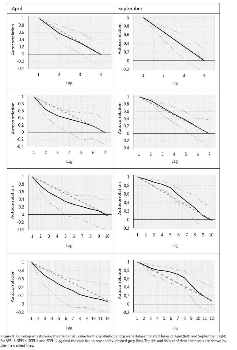
Figures 7 and 8 show how seasonality or start times can enhance or diminish the persistence of SPI (Fig. 7) and SPEI (Fig. 8) at Langgewens. The figures show the median value of AC computed from the 100 synthetic datasets where seasonality was retained for the start times of April and September for the various accumulation periods. The 95% confidence limits on the AC (shown by the dotted lines in Figs 7 and 8) were computed by ranking the AC values across the 100 synthetic datasets for a given lag time and using the min and max values as the upper and lower limit. The straight, dashed lines in Figs 7 and 8 show the AC of the various indices for the case of no seasonality. Taking a start time of April, the AC values drop off quickly at increasing lag times, even quicker than in the case of no seasonality. In contrast, when selecting a start time of September, the AC values remain higher for several months (or lag times). In other words, the 'memory' of the dry (non-rainfall) season was quickly lost, and the AC dropped off rapidly. As such, if dry conditions occur at the start of the rainy season, the greater variability between the 'dry' and 'wet' months delivers an opportunity to break these dry conditions (Lyon et al., 2012). In contrast, if dry conditions occur in the dry season, there is minimal opportunity to alleviate these conditions due to the relatively low rainfall variability during the dry season. Thus, in regions with high rainfall seasonality, such as Langgewens, seasonality will enhance or diminish the predictability of SPI and SPEI, depending on the start time. This tendency is more pronounced at longer intervals such as SPI 9 or SPI 12. This makes these two accumulation periods useful for seasonal predictions. In addition, when comparing SPEI (Fig. 8) with SPI (Fig. 7), SPEI shows the same trends as SPI but has slightly diminished AC for 6- and 9-month accumulation periods for a September start time.

Variations in persistence

Seasonal changes in persistence characteristics of SPI and SPEI indices for both stations are shown in Table 2. The results were obtained from the 100 synthetic datasets where seasonality was retained. Results showed persistence varied, with the greatest persistence observed in the longer accumulation periods of SPI 9 or SPEI 9 and SPI 12 or SPEI 12. There is a large discrepancy between persistence at Langgewens from 3-8 months, depending on the start time considered. The greatest accumulation periods were for spring for Langgewens, with lag times of up to 8 months. The lowest persistence at Langgewens was for autumn.

For the Outeniqua station, persistence characteristics are similar between seasons, aside from spring which shows the lowest persistence. Referring to Fig. 2 as well as Engelbrecht et al. (2015), this is explained because spring contributes the most to the total annual rainfall, and thus rainfall variability in spring will be the highest. Results from Roffe et al. (2021) show evidence of trends towards an increase in the degree of seasonality concentrated around the winter months for the Cape south coast. This suggests that this methodology may become more applicable in this region in the future. Since SPEI does not appear to have any benefits over SPI for Langgewens, for the rest of the analysis, the rest of the study will focus on the use of SPI. However, the principles documented will also apply to SPEI.

Baseline probabilities for the Western Cape

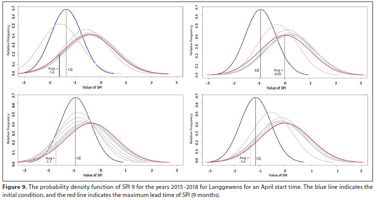
The previous sections illustrate that persistence of drought indices can provide valuable predictive information for several months of lead time. These persistence characteristics can also be utilised to determine PDFs for any given, observed, initial condition (Lyon et al., 2012; Behrangi et al., 2015). Because only the inherent persistence characteristics of drought indicators are considered, these PDFs provide baseline probabilities. Figure 9 shows PDFs for SPI 9 for a start time of April at 9 months lead time for 20152018. The study chose an April start time because it gives a more reliable or predictable PDF at each lag time than a September start time. This is because SPI 9 in April captures accumulation over the dry season from August- April. In contrast, SPI 9 in September (accumulating over January-September) contains the wet season. Figure 9 shows that the distribution at short lead times (1-3 months) is narrower than that at longer leads (6-9 months). This is due to the influence of the climatological mean at longer lead times. This allows for a 'greater memory' of the initial condition at shorter lead times, while at longer lead times the PDF will tend toward its climatological distribution (Lyon et al., 2012).

For an April start time in 2015, the initial SPI 9 value is -1.4; at 4 months lead time (August 2016), SPI 9 value was -1.6. Relative to the climatological mean, the unconditional persistence 'forecast' for August 2017 indicates an enhanced probability of SPI 9 values being <0. By February or at a 9-month lead time, the PDF resembles the climatological mean. For an April start time in 2016, the initial SPI 9 value was -0.95; at 4-months lead time, SPI was -0.05. Relative to the climatological mean, the unconditional persistence 'forecast' for August 2016 indicates an enhanced probability of SPI 9 values being >0. Taking SPI 9 in 2017 for an April start time, the initial condition (value) was -1.05, and at 4 months lead time (August 2017) SPI was -1.7. Similarly, for April 2018, the initial SPI 9 was -1.2 while at 4 months lead time, SPI 9 was -1.4. Once again, the PDFs for April 2017 and 2018 show an enhanced probability of SPI 9 values being >0 for August 2017 and 2018.

Optimal persistence

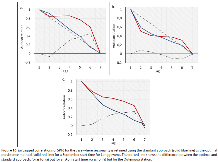
After applying the formula set out by Lyon et al. (2012) to optimise the persistence of SPI 6, the difference between optimised AC and the original AC is shown in Fig. 10 for the case of no seasonality at Outeniqua (Fig. 10c), and the case of inclusion of seasonality at Langgewens (Figs 10a and b). SPI 6 was chosen for this process because, from Fig. 7, SPI 6 and SPI 3 showed lower persistence than SPI 9 and SPI 12, so optimising for these accumulation periods is likely to bring the most benefits. Figure 10 shows that when considering only values which are shared between two accumulation periods, the persistence is higher, even in the case of no seasonality (Fig. 10c). For a September start time at both stations (Figs 10 a and c), the greatest optimisation occurs at longer lag times. For an April start time (Fig. 10b), the optimisation is greatest at shorter lags. When drought index predictions are based exclusively on persistence characteristics, the optimal persistence method is the more appropriate technique for both regions.

Behrangi et al. (2015) suggested that this methodology may be further improved by combining seasonal drought persistence characteristics with other large-scale forcing mechanisms. Results of Archer et al. (2019) and Odoulami et al. (2021) suggest that AAO/SAM may influence seasonal rainfall in the WRRWC and will thus likely enhance the predictive skill of persistence.

Cumulative distribution functions (CDF)

Figure 11 shows the CDF for SPI 9 for an April start time for the drought years 2015-2018 and the probability that SPI < -1 in October for the observed Langgewens and Outeniqua datasets. First, it should be noted that all 4 years at Langgewens show a high probability of SPI < -1. For SPI 9 in 2015, the probability of drought occurring in October was ~75%. In 2016, the probability was ~25%, 2017 showed a ~48% probability, and 2018 showed a ~30% probability. The probabilities reflect the evolution of the drought over the 4 years. According to Theron et al. (2021), the drought was most severe in 2015 and 2017 in the WRRWC.

For Outeniqua, only 2017 showed a high probability (~68%) of SPI < -1. In 2015 at Outeniqua, there was a ~22% probability of drought occurring. 2016 (~18%) and 2018 (~8%) showed the lowest probability of SPI < -1. This was expected as the Outeniqua area did not experience drought conditions in 2015 as severe as Langgewens. Both showed high drought probability in 2017 when the drought reached its maximum regional extent (Theron et al., 2021). However, Outeniqua showed a lower drought probability than Langgewens for 2018.

 

CONCLUSIONS AND RECOMMENDATIONS

The work presented here sought to apply the methodology set out by Lyon et al. (2012) to quantify the persistence characteristics of two drought indices and to establish a set of baseline probabilities for seasonal drought prediction in the WRRWC. Cumulative density functions for the 2015-2018 drought period were developed to give an indication of the methodology's potential for predicting drought. The study also aimed to determine if there was any benefit of using SPEI over SPI for this analysis. The study found that, at least for the Langgewens region, SPI showed greater persistence than SPEI. Thus, using SPI over SPEI for this application in this region may provide some predictive benefits. In addition, seasonality was able to enhance and diminish the predictability of drought at Langgewens. Selecting September (spring) as a start month for such calculations at the Langgewens station improved persistence characteristics by up to 5 months of lead time when compared with a March (autumn) start time.

However, no distinct start month improved persistence at the Outeniqua station.

The results show potential for the use of drought indices for seasonal drought prediction in the WRRWC. It is recommended that further studies be undertaken which incorporate a more extensive set of weather stations or use gridded rainfall data. Furthermore, follow-up studies should test the predictive skill and skill scores outside the case study period using cross-validation with large datasets. Finally, additional research is needed to explore how coupling drought indices with other factors such as the presence of AAO/SAM (Archer et al., 2019), El Nino 3.4, and sea-surface temperature (Behrangi et al., 2015) could improve predictive skill. The results may aid interpretation and highlight areas where this methodology can be applied within an early warning context or decision support tool for the Western Cape and highly seasonal regions in South Africa. The methodology and results also show that drought prediction can be enhanced using a simple computation and minimal data inputs. This is particularly relevant to drought-prone regions where data for more advanced computations may be scarce, such as sub-Saharan Africa.

 

DECLARATION OF COMPETING INTEREST

None.

 

ACKNOWLEDGEMENTS

This work was supported through the Agriculture Research Council's Professional Development Program (ARC-PDP). Immense gratitude is also extended to Mr A Theron who helped with the coding needed to run the methodology.

 

AUTHOR CONTRIBUTIONS

ST - conceptualisation and methodology, data collection, data analysis, interpretation of results, writing of the initial draft. EA, CE, SM, SW - revision after review.

 

ORCIDS

SN Theron: https://orcid.org/0000-0002-8895-9464

E Archer: https://orcid.org/0000-0002-5374-3866

C Engelbrecht: https://orcid.org/0000-0003-2513-2889

S Midgley: https://orcid.org/0000-0002-7916-7115

S Walker: https://orcid.org/0000-0002-7090-4860

 

REFERENCES

ARC (Agricultural Research Council) (2018) Agromet-climate database. Soil, Climate and Water, Agricultural Research Council, Pretoria.         [ Links ]

ARCHER E, LANDMAN W, MALHERBE J, TADROSS M and PRETORIUS S (2019) South Africa's winter rainfall region drought: A region in transition? Clim. Risk Manage. 25 100188. https://doi.org/10.1016/j.crm.2019.100188        [ Links ]

BEGUERÍA S, VICENTE-SERRANO SM, REIG F and LATORRE B (2014) Standardised precipitation evapotranspiration index SPEI revisited: parameter fitting, evapotranspiration models, tools, datasets and drought monitoring. Int. J. Climatol. 34 (10) 3001-3023. https://doi.org/10.1002/joc.3887        [ Links ]

BEHRANGI A, NGUYEN H and GRANGER S (2015) Probabilistic seasonal prediction of meteorological drought using the bootstrap and multivariate information. J. Appl. Meteorol. Climatol. 54 (7) 1510-1522. https://doi.org/10.1175/JAMC-D-14-0162.1        [ Links ]

BOTAI CM, BOTAI JO, DE WIT JP, NCONGWANE KP and ADEOLA AM (2017) Drought characteristics over the western cape province, South Africa. Water 9 (11) https://doi.org/10.3390/w9110876        [ Links ]

BRAUN K, BAR-MATTHEWS M, AYALON A, ZILBERMAN T and MATTHEWS A (2017) Rainfall isotopic variability at the intersection between winter and summer rainfall regimes in coastal South Africa Mossel Bay, Western Cape Province. S. Afr. J. Geol. 120 (3) 323-340. https://doi.org/10.25131/gssajg.120.3323        [ Links ]

BUURMAN J, DAHM R and GOEDBLOED A (2014) Monitoring and early warning systems for droughts: lessons from floods. SSRNElectron. J. January 2014.         [ Links ]

EDWARDS B, GRAY M and HUNTER B (2019) The social and economic impacts of drought. Aus. J. Soc. Iss. 54 (1) 22-31. https://doi.org/10.1002/ajs4.52        [ Links ]

ENGELBRECHT CJ, LANDMAN WA, ENGELBRECHT FA and MALHERBE J (2015). A synoptic decomposition of rainfall over the Cape south coast of South Africa. Clim. Dyn. 449 (10) 2589-2607. https://doi.org/10.1007/s00382-014-2230-5        [ Links ]

FAVRE A, HEWITSON B, LENNARD C, CEREZO-MOTA R and TADROSS M (2013). Cut-off lows in the South Africa region and their contribution to rainfall. Clim. Dyn. 419 (10) 2331-2351. https://doi.org/10.1007/s00382-012-1579-6        [ Links ]

GUENANG GM and KAMGA FM (2014) Computation of the standardized precipitation index (SPI) and its use to assess drought occurrences in Cameroon over recent decades. J. Appl. Meteorol. Climatol. 53 (10) 2310-2324. https://doi.org/10.1175/JAMC-D-14-0032.1        [ Links ]

HARGREAVES GH and SAMANI ZA (1985) Reference crop evapotranspiration from temperature. Appl. Eng. Agric. 1 (2) 96-99. https://doi.org/10.13031/2013.26773        [ Links ]

HENNINGSE C (2021) Personal communication, 17 June 2021. Ms Chrisna Henningse, Agricultural Research Council - Natural Resources and Engineering, 600 Belvedere Street, Arcadia, Pretoria 0083, South Africa.         [ Links ]

JOHNSTON P and WOLSKI P (2018) Will there be more rain this winter? Climate Systems Analysis Group, University of Cape Town. URL: http://www.csag.uct.ac.za/2018/03/15/will-there-be-more-rain-this-winter/ (Accessed 25 June 2020).         [ Links ]

LYON B BELL MA, TIPPETT MK, KUMAR A, HOERLING MP, QUAN XW and WANG H (2012) Baseline probabilities for the seasonal prediction of meteorological drought. J. Appl. Meteorol. Climatol. 51 (7) 1222-1237. https://doi.org/10.1175/JAMC-D-11-0132.1        [ Links ]

MASON SJ (1998) Seasonal forecasting of South African rainfall using a non-linear discriminant analysis model. Int. J. Climatol. 18 (2) 147-164. https://doi.org/10.1002/(SICI)1097-0088(199802)18:2<147::AID-JOC229>3.0.CO;2-6        [ Links ]

MIDGLEY GF, CHAPMAN RA, HEWITSON B, JOHNSTON P, DE WIT M, ZIERVOGEL G, MUKHEIBIR P, VAN NIEKERK L, TADROSS M, VAN WILGEN BW and KGOPE B (2005) A status quo, vulnerability and adaptation assessment of the physical and socio-economic effects of climate change in the Western Cape. Report to the Western Cape Government, Cape Town, South Africa. CSIR Report No. ENV-S-C 2005-073. CSIR, Stellenbosch.         [ Links ]

ODOULAMI RC, WOLSKI P and NEW M (2021) A SOM-based analysis of the drivers of the 2015-2017 Western Cape drought in South Africa. Int. J. Climatol. 41 1518-1530. https://doi.org/10.1002/joc.6785        [ Links ]

OTTO FE, WOLSKI P, LEHNER F, TEBALDI C, VAN OLDENBORGH GJ, HOGESTEEGER S, SINGH R, HOLDEN P, FUCKAR NS, ODOULAMI RC and NEW M (2018) Anthropogenic influence on the drivers of the Western Cape drought 2015-2017. Environ. Res. Lett. 13 (12) 124010. https://doi.org/10.1088/1748-9326/aae9f9        [ Links ]

PASCALE S, KAPNICK SB, DELWORTH TL and COOKE WF (2020) Increasing risk of another Cape Town "Day Zero" drought in the 21^st century. Proc. Natl Acad. Sci. 117 (47) 29495-29503. https://doi.org/10.1073/pnas.2009144117        [ Links ]

PHILIPPON N, ROUAULT M, RICHARD Y and FAVRE A (2011) The influence of ENSO on South Africa winter rainfall. Int. J. Climatol. 32 (15) 2333-2347. https://doi.org/10.1002/joc.3403        [ Links ]

REASON CJC and ROUAULT M (2005) Links between the Antarctic Oscillation and winter rainfall over western South Africa. Geophys. Res. Lett. 32 (7) L07705. https://doi.org/10.1029/2005GL022419        [ Links ]

ROFFE SJ, FITCHETT JM and CURTIS CJ (2019) Classifying and mapping rainfall seasonality in South Africa: a review. S. Afr. Geogr. J. 101 (2) 158-174. https://doi.org/10.1080/03736245.2019.1573151        [ Links ]

ROFFE SJ, FITCHETT JM and CURTIS CJ (2021) Investigating changes in rainfall seasonality across South Africa: 1987-2016. Int. J. Climatol. 41 e2031-2050. https://doi.org/10.1002/joc.6830        [ Links ]

SOUSA PM, BLAMEY RC, REASON CJ, RAMOS AM and TRIGO RM (2018) The 'Day Zero' Cape Town drought and the poleward migration of moisture corridors. Environ. Res. Lett. 13 (12) 124025. https://doi.org/10.1038/s41612-019-0084-6        [ Links ]

THERON SN, ARCHER E, MIDGLEY SJE and WALKER S (2021) Agricultural perspectives on the 2015-2018 western cape drought, South Africa: Characteristics and spatial variability in the core wheat growing regions. Agric. For. Meteorol. 304 108405. https://doi.org/10.1016/j.agrformet.2021.108405        [ Links ]

THERON SN, ARCHER ERM, MIDGLEY SJE, and WALKER S (2022) Exploring farmers' perceptions and lessons learned from the 2015-2018 drought in the Western Cape, South Africa. J. Rural Stud. 95 208-222. https://doi.org/10.1016/j.jrurstud.2022.09.002        [ Links ]

VAN NIEKERK A and JOUBERT SJ (2011) Input variable selection for interpolating high-resolution climate surfaces for the Western Cape. Water SA 37 (3) 271-279. https://doi.org/10.4314/wsa.v37i3.68475        [ Links ]

VENKATRAMANAN S, VISWANATHAN PM and CHUNG SY (eds) (2019) GIS and Geostatistical Techniques for Groundwater Science. Elsevier. https://doi.org/10.1016/C2017-0-02667-8        [ Links ]

VICENTE-SERRANO SM, BEGUERÍA S and LÓPEZ-MORENO JI (2010) A multiscalar drought index sensitive to global warming: the standardised precipitation evapotranspiration index. J. Clim. 23 (7) 1696-1718. https://doi.org/10.1175/2009JCLI2909.1        [ Links ]

WELDON D and REASON CJC (2014) Variability of rainfall characteristics over the South Coast region of South Africa. Theor. Appl. Climatol. 115 (1-2) 177-185. https://doi.org/10.1007/s00704-013-0882-4        [ Links ]

WMO (World Meteorological Organization) (2012) Standardized precipitation index user guide. WMO Report No. 1090. World Meteorological Organization, Geneva.         [ Links ]

ZARGAR A, SADIQ R, NASER B and KHAN FI (2011) A review of drought indices. Environ. Rev. 19 333-349. https://doi.org/10.1139/a11-013        [ Links ]

 

 

Correspondence:
SN Theron
Email: therons@magellanicsensing.com

Received: 24 September 2022
Accepted: 14 April 2023