


Services on Demand
Article
 English (pdf)
 Article in xml format
 Article references
Indicators

Related links
-
 Cited by Google
 -
 Similars in Google
Share

 Permalink
Water SA
On-line version ISSN 1816-7950
Print version ISSN 0378-4738
Water SA vol.48 n.4 Pretoria Oct. 2022
http://dx.doi.org/10.17159/wsa/2022.v48.i4.3977
RESEARCH PAPER
South Africa needs a hydrological soil map: a case study from the upper uMngeni catchment
JJ van ToiI; GM van ZijlII
IDepartment of Soil, Crop and Climate Sciences, University of the Free State, Bloemfontein, South Africa
IIUnit for Environmental Sciences and Management, North-West University, Potchefstroom, South Africa
ABSTRACT
Accurate hydrological modelling to evaluate the impacts of climate and land use change on water resources is pivotal to sustainable management. Soil information is an important input in hydrological models but is often not available at adequate scale with appropriate attributes for direct parameterisation of the models. In this study, conducted in three quaternary catchments in the midlands of KwaZulu-Natal, three different soil information sets were used to configure SWAT+, a revised version of the Soil and Water Assessment Tool (SWAT). The datasets were: (i) the Land Type database (currently the only soil dataset covering the whole of South Africa), (ii) disaggregation of the Land Type database using digital soil mapping techniques (called DSMART), and (iii) a dataset where DSMART were complemented by field observations and interpretations of the hydropedological behaviour of the soils (DSMART+). Simulated streamflow was compared with measured streamflow at three weirs with long-term measurements, and the impact of the soil datasets on water balance simulations was evaluated. In general, the simulations were acceptable when compared to other studies, but could be improved through calibration and including small reservoirs in the model. The DSMART+ dataset yielded more accurate simulations of streamflow in all three catchments with Nash-Sutcliffe efficiencies increasing by between 9% and 67% when compared to the Land Type dataset. The value of the improved soil maps is, however, highlighted through the enhanced spatial detail of streamflow generation mechanisms and water balance components. The internal catchment processes are represented more accurately, and we argue that South Africa needs a detailed hydrological soil map for effective water resource management.
Keywords: digital soil mapping, hydropedology, catchment processes, Soil Water Assessment, Tool (SWAT), soil water balance
INTRODUCTION
Soils play a key role in partitioning rainfall into different components of the water balance, such as overland flow, infiltration, deep drainage, and lateral flow, and also in storing and availing water for évapotranspiration. Soil information, their hydraulic properties and spatial distribution, is therefore an important input into physically based hydrological models (Beven, 1983; Worqlul et al., 2018) for effective predictions of the impacts of climate and land use change on water resources.
With enhanced computing power, spatially distributed hydrological models are capable of handling details of landscape heterogeneity better. Some models (e.g. SWAT and SWAT+) couple seamlessly with GIS interfaces such as ArcMap and QGIS (Arnold et al, 1998; Bieger et al., 2017). The models typically rely on layers of topography, land use and soil information to delineate hydrological response units (HRUs). Advances in remote sensing have resulted in improved topographical and land use data, which are freely available at adequate scale for hydrological modelling globally. On the other hand, soil information in most developing countries is seldom available at adequate scale for direct parameterisation of most models, despite sufficient evidence from the literature that more detailed soil information with more realistic hydraulic properties improves modelling accuracy and reduces parameter calibration uncertainty (e.g. Romanowicz et al., 2005; Bossa et al., 2012; Diek et al., 2014; Van Toi et al., 2015; Wahren et al., 2016; Gagkas et al., 2021; Van Toi et al, 2021).
Reasons for the lack of appropriate soil information are that soil maps are generally not produced for hydrological modelling purposes (Zhu and Mackay, 2001), and the costs and time involved in quantifying the spatial variation of important soil hydraulic properties, such as water retention characteristics and conductivity. In South Africa, the only soil database that covers the entire country is the Land Type database (Land Type Survey Staff, 1972-2002). This 30-year endeavour aimed to characterise the soil resources of South Africa (mainly for agricultural purposes), and divided the country into 7 070 'Land Types' (Paterson et al., 2015). A Land Type is an area with a homogenous combination of terrain type, climate and consequently soil distribution pattern at a scale of 1:250 000. The soil distribution pattern refers to the sequence of soils from the crest to the valley bottom, also known as the soil catena or toposequence. Each Land Type is accompanied by an inventory which contains, amongst other information, the soil forms and their percentage coverage of different terrain morphological units (TMUs). The TMUs included are the crest, cliffs, midslope, footslope and valley bottom. Efforts have been made to convert these Land Types into suitable hydrological modelling inputs, notably by Pike and Schulze (1995) for the ACRU model. In most regional modelling studies, the Land Types are considered as a single unit with lumped average soil parameters as presented, for example, in the South African Atlas of Agrohydrology and Climatology (Schulze et al., 2007). The latter is the best available dataset of soil hydrological information for South Africa and. although certainly useful for modelling of large areas, there are several limitations associated with this dataset. These limitations are discussed in detail by Van Tol and Van Zijl (2020), but in summary:
• Observation depths are limited to 1.2 m. In large areas of South Africa, soils are considerably deeper which will result in an erroneous representation of storage and flowpaths through the soils.
• The nature of the soil/bedrock interface is not described. This interface is important in partitioning infiltrated water into recharge of groundwater stores or generation of lateral flows.
• There can be considerable variation in the soils and hydraulic properties within a Land Type, ranging from deep, freely drained soils to permanently saturated soils with slow infiltration rates. This variation is not only limited to different terrain positions, but also within the same terrain morphological unit.
With the advances in digital soil mapping (DSM; McBratney et al., 2003), detailed soil information at adequate scale and format for hydrological modelling studies can now be generated at relatively low costs (e.g. Zhu and Mackay, 2001; Thompson et al., 2012; Van Tol et al., 2015; Van Zijl et al., 2016; Wahren et al., 2016; Van Zijl et al., 2020). A key advantage of DSM is that legacy soil data (such as the Land Type database), can be remapped at finer scales and improved accuracy for a specific application - in this case to serve as modelling input. Significant progress has been made to map soils through machine learning, expert knowledge and disaggregation of Land Type approaches into soil polygons (Van Zijl, 2019), as well as for hydrological purposes in South Africa (e.g. Van Zijl et al., 2016; Van Tol et al., 2020).
We argue that it is timeous to create a hydrological soil map for South Africa, using a combination of legacy soil data, expert knowledge and DSM techniques. We present a case study where streamflow was simulated in three quaternary catchments in the KwaZulu-Natal midlands. The objectives of the study were to generate improved soil information using DSM techniques and then to evaluate the contribution of this information to modelling efficiency as well as to internal catchment processes. We also provide a suggested methodology for moving towards a hydrological soil map for the whole of South Africa.
MATERIALS AND METHODS
Study area
The focus area was three quaternary catchments in the KwaZulu-Natal midlands, namely, U20A (upper uMngeni River), U20B (Lions River) and U20D (Karkloof River) (Fig. 1). The catchment areas are 299, 358 and 339 km2 for U20A, U20B and U20D, respectively. The mean annual precipitation varies from 1 250 mm/a in U20D to 850 mm/a. in the drier middle parts in U20B, with most of the rainfall received from October to March (Schulze and Lynch, 2007). Mean daily air temperatures are around 19°C during summer and 11°C during winter (Schulze and Maharaj, 2007). Natural vegetation forms part of the Midlands Grassland, Drakensberg Foothill Moist Grassland and Southern Misbelt Forests (SANBL 2006-2018). Commercial forestry and crop production are the prominent current land uses (Fig. 2).
Model, simulations, and input data
The SWAT+ model was used for simulations using the QSWAT+ (v 1.2.3) interface. SWAT+ is a completely revised version of the well-known Soil and Water Assessment Tool (SWAT; Bieger et al.. 2017; Arnold et al, 1998). SWAT is widely used to simulate water quality and quantity to predict and assess the impacts of land use, climate change, soil erosion and pollution. A comprehensive description of the SWAT model is provided by Neitsch et al. (2009) and a description of changes and updates in the SWAT+ version is provided by Bieger et al. (2017). The model is a process-based semi-distributed catchment-scale model where one of the first steps is to divide the catchment into 'hydrological response units' (HRUs). A HRU is a homogenous area in terms of soils, land use and slope. Ihc model then calculates water balance components, including overland flow, infiltration, lateral flow, percolation, évapotranspiration and discharge to the stream from each HRU. Model setups resulted in the creation of 2 814 and 3 597 HRUs for U20A, 3 831 and 4 395 HRUs for U20B, and 3 396 and 3 948 HRUs for U20D. In each catchment the first (lower) number of HRUs was for the 'Land Type' model run and the second (higher) number of HRUs was for the DSMART and DSMART+ runs (discussed in detail later). The model was run from January 1998 till December 2013 on the three catchments individually, using three levels of soil input data (i.e. 9 model runs). The different soil inputs are discussed under the soil data section. The first 2 years were used as a warm-up period, followed by 14 years of validation. As the aim was not optimization through calibration, we did not include a model calibration period.
Streamflow was recorded at Department of Water and Sanitation (DWS) weirs U2H013, U2H007 and U2H006 (Fig. 1). Daily rainfall records were obtained from 7 rainfall stations from the South African Weather Service (SAWS) and DWS (Fig. 1). The average annual rainfall recorded at these stations during our simulation time (2000-2013) was 675 mm. When a rainfall station malfunctioned, the average daily rainfall recorded at the remaining stations was used to infill the day/s without data. Daily minimum and maximum temperatures and relative humidity were obtained from the SAWS stations. The remainder of the climatic information (solar radiation and wind speed) was obtained from the Climate Forecast System Reanalysis (CFSR) project (Saha et al., 2010) by the National Center for Environmental Prediction (NCEP). Daily potential évapotranspiration was calculated using the Penman-Monteith (Monteith, 1965) approach.
Land cover data were obtained from the 2013/14 South African National Land-Cover Map (Geoterralmage, 2014, Fig. 2). Pre-defined SWAT values for different land-use classes were used as input data for the land cover. Dams were identified from the land cover and included in the model set-up as 'reservoirs' with estimated parameters. Here we only included relatively large dams (>1 ha), totalling 3, 2, and 3 for U20A, U20B and U20D respectively. Smaller ponds and farm dams were assigned default SWAT+ parameters for a 'water' land use class in the model.
Soil data
Three levels of soil input data were used: (i) the Land Type database (currently the only soil dataset covering the whole of South Africa), (ii) disaggregation of the Land Type database using digital soil-mapping techniques (called DSMART) and (iii) a dataset where DSMART were complemented by field observations and interpretations of the hydropedological behaviour of the soils (DSMART+).
Land type data
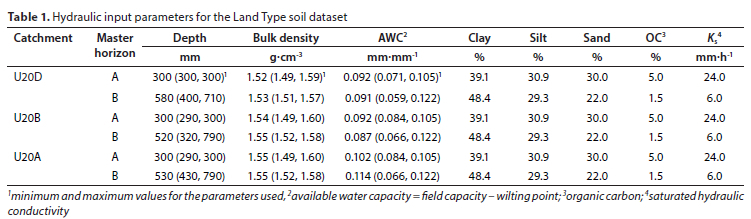
The Land Type database is the best, readily available soil dataset which covers the whole of South Africa (Land Type Survey Staff 1972-2002). A Land Type is a homogenous area in terms of climate, geology and topographical patterns, which can be mapped at a scale of 1:250 000 (Paterson et al., 2015). It is important to note that a Land Type does not represent a soil polygon but rather a soil distribution pattern. The Land Type dataset is widely used for hydrological modelling studies and efforts have been made to provide average hydraulic parameters for two soil horizons per Land Type for simulations in the ACRU hydrological model (Pike and Schulze, 1995; Schulze, 2007). There are 46 Land Types in the study area (Fig. 3). The majority of these are, however, Ac Land Types with little differences between them in terms of soil distribution patterns andhydraulic properties (Fig. 3 and Table 1). According to the Land Type inventories, A Land Types are dominated by red and yellow soils without water tables and in Ac Land Types, red and yellow soils cover more than 10% of the land area and dystrophic and/or mesotrophic soils occupy larger areas than their high-base-status counterparts (Land Type Survey Staff, 1972-2002). This implies that the soils are freely drained and leached. With exception of Ks, all the SWAT-required properties for the Land Type data are available from Schulze (2007) and are summarized in Table 1. ROSETTA (Schaap et al., 2001) was used to derive the Ks for different horizons from the texture classes. All the Land Types were assigned to the SWAT soil group A for partitioning between overland flow and infiltration, using a modified curve number method (Neitsch et al., 2009).
DSMART and DSMART+ datasets
DSMART (Odgers et al., 2014) is an automated algorithm whereby soil map units, comprising of various soil types, are disaggregated into more detailed soil classes, thereby improving the representation of the spatial distribution of the soil. Flynn adapted DSMART for disaggregation of the South African Land Types (Flynn et al., 2019a, b, c).
DSMART iteratively resamples complex polygon map units in the proportion in which they are thought to occur within the polygon, and then trains a machine-learning algorithm on the environmental covariates at the resampled sites. Thereafter it applies the trained algorithm to the entire site to produce multiple (one for each iteration) realisations (maps) of the soil distribution.
The soils within each Land Type's inventory were grouped into one of six hydropedological soil classes according to Van Tol and Le Roux (2019). Each Land Type's polygon was then divided into TMUs by merging the Land Type data layer with a TMU map of South Africa (unpublished). The proportion of each hydropedological soil group for each Land Type-TMU unit was then calculated based on the proportion given for the soil types within the Land Type inventory.
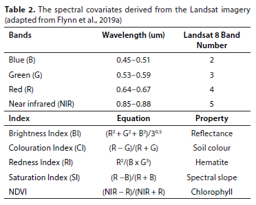
Environmental covariates collected for the site included Landsat satellite imagery taken on 20201017 as well as the Shuttle Radar Topography Mission (STRM) 30 m DEM. These sources were projected and resampled to fit onto the same grid and clipped to the size of the three catchments studied. The indices given in Table 2 were derived from the Landsat image, while the channel network base level, altitude, the LS-factor, planform and profile curvature, relative slope position, slope gradient, the topographic wetness index and valley depth were derived from the DEM.
DSMART was run using 100 samples per polygon and applying the random forest algorithm. This gave 10 hydropedological soil group maps, of which the best realisation was used as the DSMART soil map for the hydrological modelling.
For the DSMART dataset, undisturbed samples were collected of representative soil horizons. These soils were then subjected to laboratory analysis where the bulk density and hydraulic conductivity (falling head method) were determined. Data from modal profiles of the Land Type database (Fig. 4) were used to obtain average particle size distribution and organic carbon for the different soil groups. These were then used in a pedotransfer function (PTF) for South African soils (Hutson, 1984) to derive 'drained upper limit' (field capacity) and 'lower limit' (wilting point) of available water, the difference between these is the 'available water capacity' (AWC). The DSMART+ dataset also included field observations, especially regarding soil depth and the hydropedological response of the soils in the input data.
Statistical analysis
Simulated monthly streamflow was compared with measured flow at the three stream gauges (Fig. 1). Statistical comparisons were made using five widely used indices, namely, the coefficient of determination (R2), the root mean square error (RMSE), percentage bias (PBIAS), the Nash-Sutcliffe efficiency (NSE) and the Kling-Gupta efficiency (KGE).
PBIAS indicate the degree of over- or underestimation of the simulations when compared to observed values (Gupta et al., 1999):

Where Yiobs and Yisim are the observed and simulated value for a specific timestep (i), respectively. Positive values signify underestimation and negative values overestimation when compared to measured values. NSE is used to determine the magnitude of variance between simulated and observed values (Nash and Sutcliffe, 1970):

Where Yi°bs and Yisim are again the observed and simulated value at a timestep (i), Ymean is the average of the entire simulation period and n is the number of observations. In general, a value > 0.5 signifies satisfactory model performance when comparing monthly data (Moriasi et al., 2015).
The KGE is calculated using (Gupta et al., 2009):

Where r represents the correlation coefficient, σsim and σsim the standard deviation in simulations and observations, respectively, and μsim and ,μobs the means of simulations and observations. Higher KGE values indicate better model performance and a value smaller than -0.41 implies that the means of the observations provide a better fit than the model (Knoben et al., 2019).
RESULTS AND DISCUSSION
Hydropedological soil map and DSMART input parameters
The hydropedological soil map (Fig. 4), had a 61% observation point accuracy in terms of mapping the hydropedological groups. This is comparable to the accuracy of conventional soil surveys (65%, Marsman and De Gruijter, 1986) and other similar digital soil mapping products, e.g., 69% (MacMillan et al., 2010) and 73% (Van Zijl and Le Roux, 2014). The majority of the error (32%) was between mapped recharge (shallow) soils and observed recharge (deep) soils. In the Land Type inventory, saprolite was deemed a restricting layer and the total soil depth given as the thickness of soil horizons above the saprolite layer. In the study area the saprolitic layers were very thick and chemically weathered, which would contribute greatly to the storage capacity of the soil profile (Fig. 5). This will allow more water for evapotranspiration and could reduce the amount of recharge to the groundwater and increase the time it will take for groundwater recharge (Ogeen et al., 2005). In the observations these were consequently classified as recharge (deep), which contributed to the map error.
Mapped recharge (deep) but observed interflow (deep) contributed to 6% of the mapping error. Again, the observation depth limit of the Land Type dataset could be attributed to this. Gleyic or plinthic horizons below 1 200 mm were not recorded in the Land Type survey, but could play an important role in the generation of lateral flow.
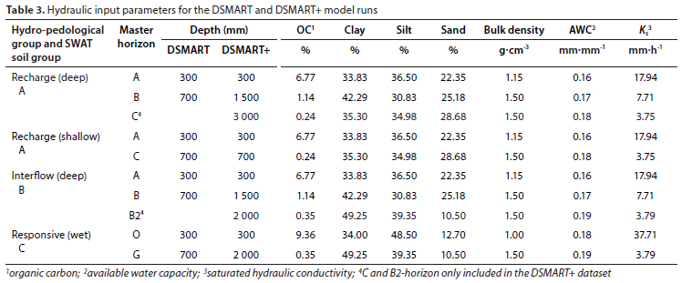
For the DSMART model runs, estimated soil parameters from the Land Type dataset and modal profiles were used (Table 3). These model inputs reflected a scenario where a field visit was not conducted and only legacy data together with digital soil mapping are available. For the DSMART+ model runs, the horizon depths were adjusted to reflect actual depths observed during the field survey (Table 3).
Streamflow predictions
The accuracy of streamflow simulations differed between different catchments and soil input levels (Table 4). Warburton et al. (2010) also conducted hydrological modelling studies in these catchments and obtained NSE values of 0.80,0.85 and 0.66 for daily streamflow simulations in U20A, U20B and U20D, respectively. This is considerably better than our predictions shown in Table 4. It should, however, be emphasised that the aim of this study was to evaluate the direct contribution/impact of soil information of simulations and not to optimize model outputs. The obtained R2 values are comparable with other similar studies, for example R2 of between 0.42 and 0.71 in West Africa (Bossa et al., 2012), R2 = 0.15 in Colorado (Diek et al., 2014) and R2 between 0.60 and 0.74 in a South African case study (Van Tol et al., 2020). Moriasi et al. (2007) recommended that 'satisfactory' simulations have NSE values > 0.5 and PBIAS values < ±25. With this as baseline, all the model runs in U20D are satisfactory in terms of NSE, but only the DSMART+ simulations were satisfactory in U20B and U20A, when the same index was considered. In terms of the PBIAS, streamflow was overestimated in all model runs and only the DSMART and DSMART+ simulations in U20B were within the 'satisfactory' range. The overestimation of streamflow is likely the result of not including small water bodies (farm dams) in the model set-up. These water bodies will first need to be filled before significant flow can occur and also contribute to evaporation, hence the overestimation of streamflow when they are omitted. Including these reservoirs associated with realistic hydraulic parameters should be a key consideration in future modelling actions.
There was a definite improvement in streamflow predictions when more detailed soil information was used (Table 4). DSMART+ predictions all had higher NSE and KGE values, whereas the RMSE and the PBIAS were closer to zero. Interestingly, the DSMART simulations performed worse than the Land Type information in U20D and U20A (if KGE is considered). In all scenarios there was an overestimation of streamflow, as indicated by the negative PBIAS values (Table 4). Land type data resulted in the highest degree of overestimation in U20D and U20B, while DSMART soil data performed worst in this regard in U20A. In all the catchments the DSMART+ soil data yielded the lowest levels of streamflow overestimation.
The improvement in streamflow simulations with improved soil information agrees with findings of other studies (e.g., Romanowicz et al., 2005; Bossa et al., 2012; Diek et al., 2014; Van Tol et al., 2015; Wahren et al., 2016; Van Tol et al., 2020, Gagkas et al., 2021). From the monthly streamflow data, there appears to be no definite trend in when streamflow is overestimated, i.e., it was overestimated during both wet and dry years (Fig. 6). During extreme events, for example, the beginning of 2009, actual streamflow exceeded predicted streamflow in all three catchments.
Water balance components
Catchment average components
There were marked differences in the water balance components in the different catchments when different soil input data were used (Table 5). U20D received the highest average annual rainfall (876 mm), followed by U20A (757 mm) then U20B (705 mm). Simulated overland flow was also the highest in U20D, whereas U20A and U20B had similar simulated overland flow volumes. The DSMART soil input yielded the highest overland flow in all catchments, followed by DMSART+ and lastly the Land Type data. The Land Type dataset provided only average soil parameters for large areas whereas the DSMART and DSMART+ datasets included soils which will be prone to overland flow generation such as responsive (wet) soils (SWAT soil group C; Neitsch et al., 2009). The average depth of soils in the DSMART dataset was shallower than that of DSMART+, explaining the higher simulated overland flow when using the former.
Simulated lateral flows were similar for the Land Type and DSMART soil inputs, but markedly lower when the DSMART+ input data were used. This could be attributed to the deeper soils in the DSMART+ dataset. Water draining vertically through the soil to the soil/bedrock interface, where lateral flow will occur, is available for plant root uptake. It will take longer for the water to drain through the deeper soils to the bedrock (Asano et al., 2002), and more water will be transpired and consequently there will be less lateral flow. This is supported by the higher transpiration rates (Table 5) when using the DSMART+ dataset. Simulated transpiration was higher, and evaporation generally lower, when usingthe DSMART+ input data compared to the othertwo datasets. The exception was U20D where the DSMART data resulted in the lowest simulated evaporation. Evapotranspiration (ET) is by far the largest water balance component, accounting for between 55% and 64% of the rainfall. Simulated percolation to groundwater was 18-25% higher in U20D when using the DSMART+ input data compared to the Land Type and DSMART soil data, although the absolute differences were relatively small (7.2 mm). The increased percolation when using the DSMART+ dataset could be attributed to less lateral flow; the soils are deeper and lateral flow not generated as easily as with the other datasets (Table 5). For the other two catchments, differences in the percolation were not noteworthy.
Average soil water storage is expressed as millimetres (mm) of available soil water for the entire profile and the top 300 mm (topsoil horizon) in Table 5. Differences in the soil water were the most pronounced of all the water balance components. For the entire profile, simulations using the DSMART+ dataset stored 194% (U20D), 673% (U20B) and 542% (U20A) more water than simulations using the Land Type dataset. Similarly, the DSMART+ dataset resulted in increased simulated soil water of 62%, 261% and 212% for U20D, U20B and U20A, respectively, compared to the DSMART dataset. The DSMART soil data also resulted in increased soil water when compared to the Land Type data; increases of 81%, 114% and 106% for U20D, U20B and U20A, respectively. Topsoil water contents showed similar trends as that of the entire profile i.e., DSMART + > DSMART > LandType. The differencesin available water in the topsoil were not as large as for the profile average water The differences in soil water content are the consequence of the soil input data (Table 1 and 2), where the deeper soils of the DSMART+ input data will have a higher storage capacity.
Water balance of different land uses
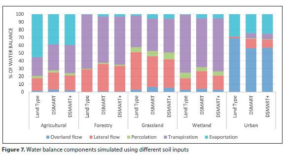
Marked differences were observed in how different soil inputs impact simulated water balance components for different land uses, as shown in Fig. 7. For agricultural land use, evaporation was the dominant component of the water balance (55%) when the Land Type data was used, followed by transpiration (24%) and lateral flow (16%). The DSMART and DSMART + input data predicted that evaporation comprised 40% and 39% of the water balance, respectively. The high evaporation is presumably related to fallow periods or evaporation between rows in planted crops. Future work should determine if these values are realistic given the shift towards residue retention to reduce evaporation. Simulated lateral flows were the highest using the DSMART dataset for agricultural, forestry, wetland and urban land uses, for the grassland (dominant land use), the Land Type dataset yielded the highest lateral flow simulations (48% of precipitation). Percolation to the groundwater was also highest in grasslands, presumably due to relatively shallow rooting depth when compared to agricultural and forestry. Water draining past the rooting zone will be able to recharge the groundwater. The Land Type dataset also resulted in the highest predicted overland flow in the urban land use (69%), compared to 56% and 57% for the DSMART and DSMART + dataset, respectively.
Spatial distribution of water balance components
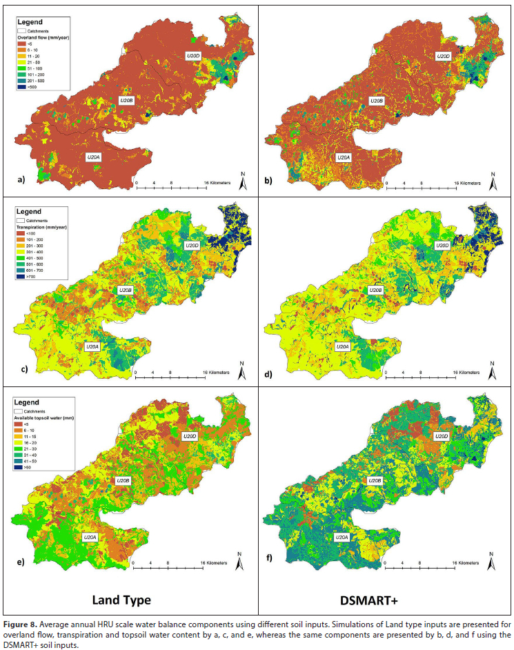
The spatial detail of water balance components using the DSMART+ is considerably higher than that using the Land Type soil inputs (e.g. Fig. 8a vs 8b). This is especially true for the soil-driven components, such as overland flow and topsoil water content (we only presented the Land Type and DSMART+ datasets to illustrate differences between datasets; similar differences in trends were observed between the Land Type and DSMART dataset). The difference in the level of detail is due to the higher number of HRUs which were generated when the detailed soil map (Fig. 4) was used. For example, in U20A, 2 779 HRUs were generated with the Land Type dataset compared to 3 597 when using the DSMART+ dataset. The spatial distribution of the different soils is also better represented in the DSMART and DSMART+ datasets than in the Land Type dataset, where the latter only use average values for large polygons.
Overland flow was higher near the stream channels in the DSMART+ dataset, leading to greater volume of overland flow simulated (Table 4). Transpiration simulations were generally higher for the DSMART+ dataset, especially along wetlands and stream channels. The largest difference was observed in simulations of the soil water content. We only show the topsoil (top 300 mm) of simulated water content (Fig. 8e and f). There are drastic differences in the total profile water content (Table 4), but this is strongly related to the soil depth assigned to the DSMART+ dataset which will result in considerably higher available water Figure 8e and f show that the topsoil water content simulated with the DSMART+ dataset is markedly higher than that simulated with the Land Type dataset. It further shows that the spatial resolution of the DSMART+ simulations are more detailed.
Although supporting data to verify the simulations of the spatial distribution of water balance components (e.g., measured soil water contents) are not available for the catchments at this stage, we believe that the detailed soil map provides an improved representation of the internal catchment structure and hence reflects the processes more accurately. Failure to represent these processes could lead to faulty conclusions and potential mismanagement of water resources (Yen et al., 2014). Reflecting internal catchment processes accurately becomes increasingly important when changes in land-use and climate are simulated (Kirchner, 2006; Arnold et al., 2015).
Pathway to a hydrological soil map for South Africa
From this work it is evident that:
• A methodology exists to create detailed soil information for large areas as input for hydrological models.
• Improved detailed soil information leads to improved modelling outcomes (DSMART vs Land Types)
• The best improvement comes with an improved soil map together with hydrological parameters for the soil mapping units (DSMART+ vs DSMART)
Creating a hydrological soil map of South Africa is possible through the use of DSM tools, which have been used in South Africa for improved hydrological modelling for fairly large areas before (Van Tol et al., 2020, Van Zijl et al., 2016, Van Tol et al., 2015). We propose a hybrid approach using both legacy soil data and data collected in dedicated field campaigns. The rough steps to create a national hydrological soil map would be:
1. Collect all available soil point data for South Africa.
2. Collect and derive the required environmental covariates for South Africa (as used in this paper).
3. Using the two datasets collected above, together with machine-learning algorithms, create a first-edition hydro-logical soil map for South Africa, complete with spatial certainty prediction.
4. Determine national and area-specific (where data is available) pedotransfer functions to determine the hydraulic parameters for the soils within the area.
5. Assign hydraulic properties to the soils mapped in Step 4. Where local PTFs exist, they are used, but where not, the national PTFs would be used.
6. Conduct specific field campaigns to collect data in priority areas where the map and PTFs are found wanting.
7. Update the map and PTFs to improve the first edition of the hydrological soil map of South Africa in a second edition.
Steps 6 and 7 should be repeated continuously to improve the mapping products and the resultant hydrological models.
CONCLUSIONS
Here we showed that improved soil information can improve streamflow predictions. Merely disaggregating existing soil data is, however, not sufficient, and needs to be supported by in-situ observations, measurements, and interpretations of the hydrological behaviour of the soils. Although the improvement in streamflow simulations is encouraging, the real benefit of the more detailed soil information is through representing internal catchment processes better. This is shown through an enhanced spatial resolution of different water balance components and streamflow generation mechanisms. We believe that the improved resolution represents how water reaches the stream channel, more accurately. Capturing these processes in hydrological models is important, especially for climate and land-use change predictions for impacts on water resources. These predictions are pivotal for sustainable water management. With the advancements of computing power and remote sensing, we simply cannot allow that the efficiency of modelling outputs is jeopardised by outdated, inadequate soil information which is not comparable with spatial resolutions of other inputs such as topography and land-use. Methods exist with which the spatial distribution of soil classes and properties can be accurately determined. We therefore argue that there is an urgent need to use the DSM methods to create user-friendly hydrological soil maps for the whole of South Africa. These maps should also be accompanied by hydrological properties of the dominant soil types forparameterisation of a range of hydrological models. These properties could be derived from locally developed pedotransfer functions (PTFs) or measured in-situ. The accuracy of these maps should also be determined through dedicated field campaigns to capture uncertainty in modelling input parameters.
ACKNOWLEDGEMENTS
The South African National Biodiversity Institute (SANBI) and the National Research Foundation (NRF) supported this study financially. The South African Weather Service provided valuable climatic data and Dr David Clark from UKZN for valuable comments and availing rainfall data of selected sites. Mrs Nancy Job of SANBI supported the project administratively and assisted with selecting the research sites.
AUTHOR CONTRIBUTIONS
JvT conceptualised the study, conducted the fieldwork and hydrological modelling. GvZ conducted digital soil mapping. JvT compiled the first draft which was reviewed by GvZ.
REFERENCES
ASANO Y, UCHIDA T and OHTE N (2002) Residence times and flow paths of water in steep unchannelled catchments, Tanakami, Japan. J. Hydrol. 261 173-192. https://doi.org/10.1016/S0022-1694(02)00005-7 [ Links ]
ARNOLD JG, SRINIVASAN R, MUTTIAH RS and WILLIAMS JR (1998) Large areahydrologic modelling and assessment, part I: Model development. /. Am. Water Resour. Assoc. 34 73-89. https://doi.org/10.1111/j.l752-1688.1998.tb05961.x [ Links ]
ARNOLD JG, YOUSSEF MA, YEN H, WHITE MJ, SHESHUKOV AY, SADEGHI AM, MORIASI DN, STEINER JL, AMATYA DM, SKAGGS RW, HANEY EB, JONG J, ARABI M and GOWDA PH (2015) Hydrological processes and model representation: impact of soft data on calibration. Trans ASABE. 58 1637 - 1660. https://doi.org/10.13031/trans.58.10726 [ Links ]
BEVEN K (1983) Surface water hydrology-Runoff generation and basin structure. Rev Geophys. 21 721-730. https://doi.org/10.1029/RG021i003p00721 [ Links ]
BIEGER K, ARNOLD JG, RATHJENS H, WHITE MJ, BOSCH DD, ALLEN PM and SRINIVASAN R (2017) Introduction to SWAT+, a completely restructured version of the soil and water assessment tool. J. Am. Water Resour. Assoc. 53 115-130. https://doi.org/10.1111/1752-1688.12482 [ Links ]
BOSSA AY, DIEKKRUGER B, IGUE AM and GAISER T (2012) Analyzing the effects of different soil databases on modelling of hydrological processes and sediment yield in Benin (West Africa) Geoderma. 173 61-74. https://doi.Org/10.1016/j.geoderma.2012.01.012 [ Links ]
DIEK S, TEMME AJAM and TEULING AJ (2014) The effect of spatial soil variation on the hydrology of a semi-arid Rocky Mountain catchment. Geoderma. 235 113-126. https://doi.Org/10.1016/j.geoderma.2014.06.028 [ Links ]
FLYNN T, DE CLERCQ W, ROZANOV A and CLARKE C (2019a) High-resolution digital soil mapping of multiple soil properties: an alternative to the traditional field survey? S. Afr. J. Plant Soil. 36 1-11. https://doi.org/10.1080/02571862.2019.1570566 [ Links ]
FLYNN T, ROZANOV A, DE CLERCQ W, WARR B and CLARKE C (2019b) Semi-automatic disaggregation of a national resource inventory into a farm-scale soil depth class map. Geoderma. 337 1136-1145. https://doi.Org/10.1016/j.geoderma.2018.11.003 [ Links ]
FLYNN T, VAN ZIJL G, VAN TOL J, BOTHA C, ROZANOV A, WARR B AND CLARKE C (2019c). Comparing algorithms to disaggregate complex soil polygons in contrasting environments. Geoderma. 352 171-180. https://doi.Org/10.1016/j.geoderma.2019.06.013 [ Links ]
GEOTERRAIMAGE (2014) 2013-2014 South African National Land-Cover Dataset. Report created for Department of Environmental Sciences. DEA/CARDNO SCPF002: Implementation of Land Use Maps for South Africa. Department of Environmental Affairs, Pretoria. [ Links ]
GAGKAS Z, LILLY A and BAGGALEY NJ (2021) Digital soil maps can perform as well as large-scale conventional soil maps for the prediction of catchment baseflows. Geoderma. 400 115230. https://doi.org/10.1016/j.geoderma.2021.115230 [ Links ]
GUPTA H V SOROOSHIAN S and YAPO PO (1999) Status of automatic calibration for hydrologic models: Comparison with multilevel expert calibration. J. Hydrol. Eng. 4 (2) 135-143. https://doi.org/10.1061/(ASCE)1084-0699(1999)4:2(135) [ Links ]
GUPTA HV, KLING H, YILMAZ KK and MARTINEZ GF (2009) Decomposition of the mean squared error and NSE performance criteria: Implications for improving hydrological modelling. J. Hydrol. 377 80-91. https://doi.Org/10.1016/j.jhydrol.2009.08.003 [ Links ]
KIRCHNER JW (2006) Getting the right answers for the right reasons: Linking measurements, analysis, and models to advance the science of hydrology. Water Resour. Res. 42 W03S04. https://doi.org/10.1029/2005WR004362 [ Links ]
KNOBEN WJM, FREER JE and WOODS RA (2019) Technical note: Inherent benchmark or not? Comparing Nash-Sutcliffe and Kling-Gupta efficiency scores. Hydrol. Earth Syst. Sci. 23 4323-4331. https://doi.org/10.5194/hess-23-4323-2019 [ Links ]
LAND TYPE SURVEY STAFF (1972 2002) Land Types of South Africa: Digital Map (1:250 000 scale) and Soil Inventory Datasets. ARC-Institute for Soil, Climate and Water, Pretoria. [ Links ]
MACMILLAN RA, MOON DE, COUPE RA, and PHILLIPS N (2010) Predictive ecosystem mapping (PEM) for 8.2 million ha of forestland, British Columbia, Canada. In: Boettinger JL, Howell DW, Moore AC, Hartemink AE and Kienast-Brown S (eds.) Digital Soil Mapping; Bridging Research, Environmental Application and Operation. Springer, Dordrecht, https://doi.org/10.1007/978-90-48l-8863-5_27 [ Links ]
MARSMAN BA and DE GRUIJTER JJ (1986) Quality of soil maps, a comparison of soil survey methods in a study area. Soil Survey Papers No. 15. Netherlands Soil Survey Institute, Stiboka, Wageningen. [ Links ]
MCBRATNEY AB, MENDOCA SANTOS ML and MINASNY B (2003) On digital soil mapping. Geoderma. 117 3-52. https://doi.org/10.1016/S0016-7061(03)00223-4 [ Links ]
MONTEITH JL (1965) Evaporation and environment. In: Fogg GE (ed.) Symposium of the Society for Experimental Biology, The State and Movement of Water in Living Organisms, Vol. 19. 205-234. Academic Press, Inc., NY. [ Links ]
MORIASI D, ARNOLD J, VAN LIEW M, BINGNER R, HARMEL R and VEITH T (2007) Model evaluation guidelines for systematic quantification of accuracy in watershed simulations. Trans. ASABE. 50 (3) 885-900. http://doi.org/10.13031/2013.23153 [ Links ]
NASH JE and SUTCLIFFE JV (1970) River flow forecasting through conceptual models: Part 1 A discussion of principles. /. Hydrol. 10 (3) 282-290. https://doi.org/10.1016/0022-1694(70)90255-6 [ Links ]
NEITSCH SL, WILLIAMS J, ARNOLD J and KINIRY J (2009) Soil and Water Assessment Tool Theoretical Documentation Version 2009. Texas Water Resources Institute, College Station TX USA. [ Links ]
ODGERS NP, SUN W, MCBRATNEY AB, MINASNY B and CLIFFORD D (2014) Disaggregating and harmonising soil map units through resampled classification trees. Geoderma. 214-215 91-100. https://doi.Org/10.1016/j.geoderma.2013.09.024 [ Links ]
O'GEEN AT, MCDANIEL PA, BOLL J and KELLER (2005) Paleosols as deep regolith: Implications for ground-water recharge across a loessial climosequence. Geoderma. 126 (1-2) 85-99. https://doi.org/10.1016/j.geoderma.2004.11.008 [ Links ]
PATERSON G, TURNER D, WIESE L, VAN ZIJL G, CLARKE C and van TOL J (2015) Spatial soil information in South Africa: situational analysis, limitations and challenges S. Afr. J. Sci. 111 (5/6). https://doi.org/10.17159/sajs.2015/20140178 [ Links ]
PIKE A and SCHULZE R (1995) AUTOSOILS: A program to convert ISCW soils attributes to variables usable in hydrological models. Department of Agricultural Engineering, University of Natal, Pietermaritzburg. [ Links ]
QUINN T, ZHU AX and BURT JE (2005) Effects of detailed soil spatial information on watershed modelling across different model scales. Int. J. Appl. Earth Obs. Geoinf. 7 324-388. https://doi.Org/10.1016/j.jag.2005.06.009 [ Links ]
ROMANOWICZ AA, VANCLOOSTERA M, ROUNSEVELB M and LA IUNESSEB I (2005) Sensitivity of the SWAT model to the soil and land use data parametrisation: A case study in the Thyle catchment, Belgium. Ecol. Model. 187 27-39. https://doi.0rg/l0.l0l6/j.ecolmodel.2005.01.025 [ Links ]
SAHA S, MOORTHI S, PAN HL, WU X, WANG J, NADIGA S, TRIPP P, KISTLER R, WOOLLEN J, BEHRINGER D and CO-AUTHORS (2015) The NCEP climate forecast system reanalysis. Bull. Am. Meteorol. Soc. 91 1015-1057. [ Links ]
SCHAAP MG, LEIJ FJ and VAN GENUCHTEN, MT (2001) ROSETTA, a computer program for estimating soil hydraulic parameters with hierarchical pedotransfer functions. J. Hydrol. 251 163-176. https://doi.org/10.1016/S0022-1694(01)00466-8 [ Links ]
SANBI (South African National Biodiversity Institute) (2006-2018) In: Mucina L, Rutherford MC and Powrie LW (eds) The Vegetation Map of South Africa, Lesotho and Swaziland. 2018 Version. URL: http://bgissanbiorg/Projects/Detail/186 [ Links ]
SCHULZE RE (2007) Soils: agrohydrological information needs, information sources and decision support. In: Schulze RE (ed.) South African Atlas of Climatology and Agrohydrology. WRC Report No. 1489/1/06, Section 41. Water Research Commission, Pretoria. [ Links ]
SCHULZE RE and LYNCH SD (2007) Annual precipitation In: Schulze RE (ed.) South African Atlas of Climatology and Agrohydrology. WRC Report No. 1489/1/06, Section 62. Water Research Commission, Pretoria. [ Links ]
SCHULZE RE and MAHARAJ M (2007) Mean annual temperature In: Schulze RE (ed.) South African Atlas of Climatology and Agrohydrology. WRC Report No. 1489/1/06, Section 72. Water Research Commission, Pretoria. [ Links ]
THOMPSON JA, ROECKER S, GUNWALD S and OWENS PR (2012) Digital soil mapping: Interactions with and applications for hydropedology. In: Lin HS (ed.) Hydropedology: Synergistic Integration of Soil Science and Hydrology. Elsevier, Amsterdam. 665-709. https://doi.org/10.1016/B978-0-12-386941-8.00021-6 [ Links ]
VAN TOL J J and LE ROUX PAL (2019) Hydropedological grouping of South African soil forms. S. Afr. J. Plant Soil. 36 233-235. https://doi.org/10.1080/02571862.2018.1537012 [ Links ]
VAN TOL JJ, VAN ZIJL GM, RIDDELL ES and FUNDISI D (2015) Application of hydropedological insights in hydrological modelling of the Stevenson Hamilton Research Supersite, Kruger National Park South Africa. Water SA. 41 525-533. https://doi.org/10.4314/wsa.v41i4.12 [ Links ]
VAN TOL JJ, VAN ZIJL GM and JULICH S (2020) Importance of detail soil information for hydrological modelling in an urbanised environment. Hydrology. 7 34. https://doi.org/10.3390/hydrology7020034 [ Links ]
VAN TOL JJ and VAN ZIJL GM (2020) Regional soil information for hydrological modelling. The Water Wheel April 2021. [ Links ]
VAN TOL JJ, BIEGER, K and ARNOLD JG (21) A hydropedological approach to simulate streamflow and soil water contents with SWAT+. Hydrol. Process, https://doi.org/10.1002/hyp.14242 [ Links ]
VAN ZIJL GM (2019). Digital soil mapping approaches to address real world problems in southern Africa. Geoderma. 337 1301-1308. https://doi.Org/10.1016/j.geoderma.2018.07.052 [ Links ]
VAN ZIJL GM, VAN TOL J J, BOUWER D, LORENTZ SA and LE ROUX PAL (2020) Combining historical remote sensing, digital soil mapping and hydrological modelling to produce solutions for infrastructure damage in Cosmo City, South Africa. Remote Sens. 12 433. https://doi.org/10.3390/rsl2030433 [ Links ]
VAN ZIJL GM, VAN TOL JJ and RIDDELL ES (2016) Digital mapping for hydrological modelling In: Zhang G, Brus D, Liu F, Song X and Lagacherie P (eds) Digital Soil Mapping Across Paradigms. Scales and Boundaries. Springer, Singapore. 115-129. https://doi.org/10.1007/978-981-10-0415-5_10 [ Links ]
WARBURTON ML, SCHULZE, RE and JEWITT GPW (2010) Confirmation of ACRU model results for the application in land use and climate change studies Hydrol. Earth Syst. Sci. 14 2399-2414. https://doi.org/10.5194/hess-14-2399-2010 [ Links ]
WAHREN FT, JÜLICH S, NUNES JP, GONZALEZ-PELAYO O, HAWTREE D, FEGER KH and KEIZER JJ (2016) Combining digital soil mapping and hydrological modelling data in a data scarce watershed in north-central Portugal. Geoderma. 264 350-362. https://doi.Org/10.1016/j.geoderma.2015.08.023 [ Links ]
WORQLUL AW, AYANA EK, YEN H, JEONG J, MACALISTER C TAYLOR R, GERIK TJ and STEENHUIS, TS (2018) Evaluating hydrologic responses to soil characteristics using SWAT model in a paired-watersheds in the Upper Blue Nile Basin. Catena. 163 332-341. https://doi.org/10.1016/jxatena.2017.12.040 [ Links ]
YEN H, BAILEY RT, ARABI M, AHMADI M, WHITE MJ and ARNOLD JG (2014) The role of interior watershed processes in improving parameter estimation and performance of watershed models. J. Environ. Qual. 43 1601-1613. https://doi.org/10.2134/jeq2013.03.0110 [ Links ]
ZHU AX and MACKAY DS (2001) Effects of spatial detail of soil information on watershed modelling. J Hydrol. 248 54-77. https://doi.org/10.1016/S0022-1694(01)00390-0 [ Links ]

