


Services on Demand
Article
 English (pdf)
 Article in xml format
 Article references
Indicators

Related links
-
 Cited by Google
 -
 Similars in Google
Share

 Permalink
Water SA
On-line version ISSN 1816-7950
Print version ISSN 0378-4738
Water SA vol.48 n.3 Pretoria Jul. 2022
http://dx.doi.org/10.17159/wsa/2022.v48.i3.3884
RESEARCH PAPER
Assessment of multiple precipitation interpolation methods and uncertainty analysis of hydrological models in Chaohe River basin, China
Binbin GuoI, II, III; Jing ZhangI; Tingbao XuIII; Yongyu SongI; Mingliang LiuI; Zhong DaiII
IBeijing Laboratory of Water Resources Security, Capital Normal University, Beijing 100048, China
IICollege of Geography and Tourism, Hengyang Normal University, Hengyang 421002, China
IIIFenner School of Environment and Society, The Australian National University, Canberra, ACT 2601, Australia
ABSTRACT
Precipitation interpolation is widely used to generate continuous rainfall surfaces for hydrological simulations. However, increasing the precision of values at the unknown points generated by different spatial interpolation methods is challenging. This study used the Chaohe River Basin, which is an important source of Beijing's drinking water, as a research area to comprehensively evaluate several precipitation interpolation methods (Thiessen polygon, inverse distance weighting, ordinary kriging and ANUSPLIN) for inputs in hydrological simulations. This research showed that the precipitation time-series surface generated using the ANUSPLIN interpolation method had higher accuracy and reliability. Using this precipitation input to drive the hydrological models, we explored the parameter uncertainties of four typical hydrological models (GR4J, IHACRES, Sacramento and MIKE SHE) based on the multi-objective generalized likelihood uncertainty estimation (GLUE) method. The GLUE method was used to study the parameter sensitivity and uncertainty of the model. Results showed that the ANUSPLIN precipitation interpolation surface combined with the Sacramento model performed best. The multi-objective GLUE method had obvious advantages in parameter uncertainty analysis in hydrological models. Simultaneously exploring the convex line and point density distributions of the behavioural parameters with multi-objective functions determined their distribution and sensitivity more effectively.
Keywords: precipitation interpolation, ANUSPLIN, hydrological model, uncertainty, multi-objective method
INTRODUCTION
Precipitation interpolation is a process for generating a spatially continuous distribution of precipitation over a surface grid using spatial interpolation, based on the precipitation observations of meteorological stations. Precipitation interpolation is the most commonly used method for estimating precipitation at unknown spatial locations. However, rainfall is significantly affected by topography, and the values at the unknown points generated by different spatial interpolation methods are quite different. Under some weather conditions, it is difficult to obtain accurate precipitation distribution values if the distribution of meteorological stations is sparse. Therefore, it is necessary to systematically study the principles of existing interpolation methods and explore new methods.
Spatial interpolation is the most commonly used method to estimate the precipitation of unknown spatial location points in areas where meteorological stations are sparse. However, there are large differences in the values at unknown points generated by different spatial interpolation methods. With the development of geographic information technology and its application in various fields, many researchers have studied the advantages and disadvantages of precipitation interpolation methods. The Thiessen polygon method (Thiessen, 1911; Te Chow et al., 1988) requires that the meteorological stations are relatively dense, and the topography of the interpolated areas is similar. The inverse distance weighting method (IDW) (Philip and Watson, 1982) determines the location of the unknown point position based on the linear weight combination of the sampling points. Both the IDW method and the Thiessen polygon method are geometric approaches, and both are widely used for precipitation interpolation. However, in most situations, these two methods do not capture the impact of terrain on precipitation well, as the rain gauges are generally not distributed adequately. Kriging (Oliver and Webster, 1990) is a geostatistical method, and the ordinary kriging method is similar to the IDW method, whereby the prediction of the unmeasured position is obtained by weighting the measured values around it. The ANUSPLIN (Hutchinson and Xu, 2013) interpolation model, a thin-plate smoothing spline approach, is a function method that interpolates precipitation as a function of latitude, longitude and elevation, and can effectively simulate the influence of terrain on precipitation.
These interpolation methods are widely used in the meteorological and hydrological fields. Croke et al. (2011) used the Thiessen and IDW methods to estimate the gauged and satellite-derived rainfall in the Brahmani Basin in India, and used the rainfall estimations to construct separate hydrological models of the region, finding that IDW was better than the Thiessen method, and the IDW approach weighted by the satellite data worked best. Haberlandt (2007) compared the performance of the kriging method, cokriging method indicated by radar data, the nearest neighbour method, Thiessen polygon method, IDW, ordinary kriging and the ordinary indicator kriging method through the interpolation of hourly precipitation in a large-scale extreme precipitation event that triggered a flood disaster in Germany, and found that cokriging and radar performed best. Szcześniak and Piniewski (2015) compared the applicability of the nearest neighbour, the Thiessen polygon, IDW and ordinary kriging methods in the SWAT model of the Sulejów Reservoir Basin in Poland, and found that the ordinary kriging method was superior to other methods. ANUSPLIN considers the influence of terrain on precipitation and can obtain good precipitation interpolation results. Data products generated by ANUSPLIN interpolation are widely used across the world. The topography of China is complex and varied. Hong et al. (2005) adopted ANUSPLIN to generate grid datasets of monthly mean temperature and precipitation for China (resolution 0.01°: about 1 km). The daily precipitation grid data (resolution 0.5°) provided by the China Meteorological Administration is also generated by ANUSPLIN interpolation.
Due to the complexity of hydrological processes and the limitations of human cognition, uncertainties are often present in hydrological models. The parameter uncertainties of hydrological models originating from the non-linearity of the hydrologic model structure and the correlation among various parameters of the model may lead to multiple optimum parameter sets (local optimal solutions) in the model after parameter optimization. As a result, the phenomenon of 'equifinality of different parameter sets' (Beven, 1996) exists in parameter calibration. The multi-objective GLUE method (Christiaens and Feyen, 2002) can comprehensively analyse the uncertainty of hydrological model parameters in each state during hydrological simulation, and has obvious advantages in parameter uncertainty analysis in hydrological models.
The objectives of this study were to: (i) analyse and compare the applicability of the four precipitation interpolation methods (Thiessen polygon, IDW, ordinary kriging, and ANUSPLIN) for hydrological modelling at the local basin scale in the Chaohe River basin; (ii) investigate parameter uncertainty in hydrological models based on multi-objective GLUE for four hydrological models, and (iii) explore the sensitivity of the parameters with indicators of NSElog and NSE as the objective functions in varied models.
METHODS
Study area
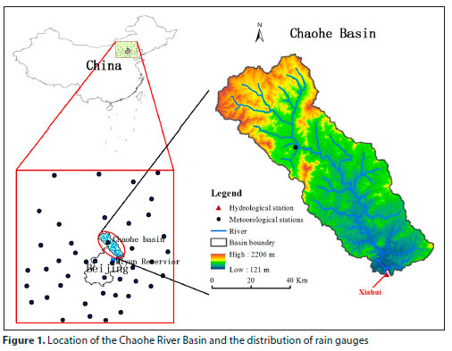
The Chaohe River Basin is located in the northeast of Beijing. It is an important water source for the Miyun Reservoir and plays a key role in the conservation of the Beijing-Tianjin-Hebei region's water source. The Miyun Reservoir provides 70% of the drinking water for Beijing and surrounding townships (population > 19 million), and about 60% of its water comes from the Chaohe River basin. The basin climate is a temperate continental monsoon climate with semi-arid characteristics. According to statistics from 1961 to 2016, the average annual rainfall of the basin is 500 mm, and the average annual evapotranspiration is 964 mm. The basin (116°-118° E, 40°-42° N) covers an area of 5 340 km2. The altitude ranges from 121 m to 2 206 m (see Fig. 1), and the mountain area accounts for 80% of the total area. Taking the catchment area above the Xiahui Hydrological Station at the watershed outlet as the study area, the drainage area is 4 815 km2.
Data acquisition
A comparative study of the four interpolation methods was carried out with data from 43 national meteorological stations around the Chaohe River. We explored the precipitation interpolation method that best reflected the eco-hydrological processes in the Chaohe River Basin and obtained the best eco-hydrological simulation results. The meteorological data came from the China Meteorological Data Network (http://data.cma.cn/). The runoff data from the Xiahui hydrological station came from the hydrological yearbook. The location of the Chaohe River Basin and the distribution of the 43 meteorological sites are shown in Fig. 1. The density of meteorological stations in the study area varies (Fig. 2), which is likely to have an impact on the results of the precipitation assessment. The kernel density (KD) function generates a smooth surface that evaluates the density of the precipitation stations by calculating the density of features around the element.
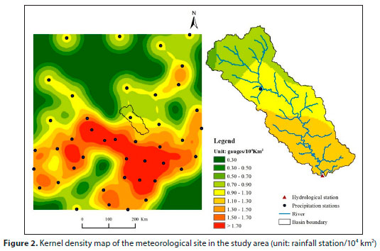
The results of the KD function are expressed as the intensity per unit area and are often used to assess the density of precipitation stations (Szcześniak and Piniewski, 2015). The meteorological station density maps in this study were generated using the kernel density estimation tool in ArcGIS Spatial Analyst (ESRI, 2012). The search radius (bandwidth) was set to 100 km. While evaluating the density of meteorological stations, the population field is set to 'none' in ArcGIS as all stations' data records are complete. Since this study was mainly aimed at comparing regional rainfall assessment methods when meteorological sites are sparse, the study area was chosen with a low density of meteorological sites (especially in the northern region), and this low-density site distribution led to a local 'hotspot' in the southern part of the density map.
Precipitation interpolation methods
The prediction of regional precipitation using the Thiessen polygon method, as shown approximately in the detail in Fig. 3, was performed by dividing the watershed into several polygons, with each polygon containing one sample point (Thiessen, 1911; Te Chow et al., 1988). Each interpolation point was determined by the value of the nearest sample point. The Thiessen polygon method is a geometric method that has the advantage of being simple and easy to implement. The disadvantage is that it often ignores information from other adjacent points and does not create a continuous precipitation surface. The Thiessen polygon method is only suitable for precipitation interpolation in relatively flat areas. However, where the rainfall time-series observed by the station is discontinuous (there may be interruptions for various reasons), the dynamic Thiessen polygon method can make full use of all available precipitation data information. In this study, the dynamic Thiessen polygon method was used to create the precipitation surface.
The Inverse distance weighting (IDW) interpolation method determines the unknown point cell values by a linear weight combination of a set of sample points. The weight is defined as a function that decreases as distance increases. It is based on the first law of geography: everything is related, but things with similar spatial locations are more closely related (Tomczak, 1998). The value at the unknown point can be approximated by the weighted sum of the values of n known points. This method assigns a larger weight to the point closest to the predicted position, and the weight decreases as the distance between the known point and the unknown point increases, so it is called the inverse distance weighting method (Philip and Watson, 1982). The IDW method is also geometric, and the method is also only applicable to areas where the topography is relatively flat.
The ordinary kriging method is similar to the IDW method. The ordinary kriging method is a geostatistical method that provides an unbiased estimate of the unobserved position based on observations from a nearby location. Ordinary kriging is one of the most commonly used kriging techniques and is characterized by an unknown and continuing trend. Ordinary kriging estimates the unknown value at a given location as a weighted linear combination of adjacent observations. The main goal of the ordinary kriging method is to define the spatial correlation to get the best estimate of the surface fitting analysis process. In this study, we used a common semi-variogram model, which can accurately simulate the spatial relationship of input sampling points or the spatial variation of discrete degrees. In the actual simulation, the semi-variogram value was dynamically calculated from the input data.
The ANUSPLIN interpolation method uses thin-plate spline interpolation technology to interpolate precipitation as a function of latitude, longitude and elevation. Therefore, ANUSPLIN can simulate the effects of topography on precipitation. In this study, ANUSPLIN 4.4 (Hutchinson and Xu, 2013) was used. ANUSPLIN is a software package based on a thin plate smoothing spline algorithm developed by the FORTRAN program. It is suitable for fitting (interpolating) surfaces to noisy data (especially climate data). The process of interpolating the data points to the grid surface is similar to the process of equation solving in which one or more independent variables exist. The partial spline model calculates the interpolated values at the position based on n observed data values as follows:
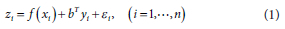
where f is the unknown smoothing function of xi, yi is a set of p-dimensional functions of independent covariates, and bT is a set of unknown p-dimensional parameters of coefficients of yi . Each εi is an independent, zero-mean error term, and the covariance can be calculated from:
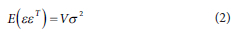
where εi = (ε1, …, εn)T, V is a positive definite n × n matrix, σ 2 can be known or unknown. If V is a diagonal matrix, the error term εi is irrelevant (Hutchinson 1995).
The function f and the coefficient b are determined by the least-squares method:
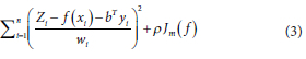
In the above formula, ρ is a smoothing parameter which is mainly used to balance data fidelity and surface roughness and the value is usually positive, Јm (f ) is the roughness measurement function of f (xi), defined as the m-order partial derivative of f (xi). The m value indicates the number of roughness occurrences, which is also called the number of splines in ANUSPLIN.
Hydrological models
The GR4J (modèle du Génie Rural à 4 paramètres Journalier) model (Perrin et al., 2003) is a lumped conceptual rainfall-runoff model with four parameters, an improved version of the GR3J model developed by Edijatno et al. (1999). The model uses rainfall and potential evapotranspiration data as input data and uses two nonlinear reservoirs for production and sink calculations. The flow module of this model for storage on the surface of the soil combines the processes of storing rainfall, evaporation and infiltration.
The IHACRES (Identification of Hydrographs and Components from Rainfall, Evaporation and Streamflow data) rainfall-runoff model was developed to help hydrology and water resources engineers to explore the dynamic relationship between rainfall and runoff and its regional characteristics, flow forecasting in ungauged watersheds, and the impacts of land-use change and climate change on the amount and distribution of runoff (Andrews et al., 2011).
The Sacramento rainfall-runoff model was developed by Burnash et al. (1973). It is currently used by the National Weather Service River Forecast Center. The version used here had 13 parameters, the ranges of which were taken from Blasone et al. (2008) (see Table 1c). The model is widely used in research. The Sacramento model uses soil moisture accounting for water balance calculations. The soil moisture store is filled by rainfall and reduced by evaporation or from the store. The excess rainfall becomes runoff that is calculated by the unit hydrograph, and the lateral flow from the soil moisture store is superimposed on this runoff and converted into streamflow (Podger et al., 2004).
The MIKE SHE model is an integrated hydrological and water resources simulation system with a comprehensive, deterministic and practical physical meaning, and is designed for all hydrological problems in river basin hydrology and water resources analysis. The model divides the watershed into discrete grids of equal area in the horizontal direction, and the vertical direction is stratified according to the geological conditions. Today, MIKE SHE has an advanced and flexible hydrological simulation framework that covers most of the processes in the hydrological cycle (Vansteenkiste et al., 2014; Vrebos et al., 2014).
GLUE methods
The GLUE method assumes that the parameters of the model are random variables subject to a joint distribution, and then calculates the posterior probability distribution of the parameters and the confidence interval of the prediction quantity through a series of measured samples, to obtain the prediction probability of the output variable. The GLUE method emphasizes the combination of model parameters, rather than a single parameter of the model, which determines the pros and cons of the model simulation results (Guo et al., 2018).
The GLUE method has three main characteristics. First, when the total number of parameter samples is large enough, the spatial distribution features of the samples are in good agreement with the spatial distribution features of the parameters. When the quantity is insufficient, there will be some difference between them. Second, the method is easily constrained by subjective factors when selecting the likelihood function and critical threshold, which may influence the simulation results. Third, this method can solve the uncertainty caused by 'equifinality'. Even if there are multiple high-probability density spaces in the parameter space, the model will not fall into the local optimal interval.
Model performance criteria
To evaluate the applicability of different precipitation prediction methods for hydrological models, the applicability of these models in watershed simulations, and the likelihood function values in the uncertainty analysis, the Nash efficiency coefficient was selected as a model evaluation index. The Nash efficiency coefficient NSE (Nash and Sutcliffe, 1970) with an optimal value of 1 is defined as follows:
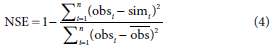
where simi and obsi represent the time-series of simulated value and observed value, respectively; obs represents the average observed values.
The NSE is a form of mean square error, an evaluation index widely used for hydrological modelling, and is often used as an objective function for the calibration of hydrological models. The range of NSE is (−∞, 1), where 1 indicates a perfect fit of the observed flow and the simulated flow. In the calibration of hydrological models, the NSE objective function can fit the high flow rate well, while the performance of the low flow rate will be relatively poor (Krause et al., 2005). The logarithmic-transformed NSE (NSElog) is proposed to increase the sensitivity to the accuracy of low-flow simulations (Oudin et al., 2006). In this study, both the NSE and the NSElog were selected as objective functions for GLUE uncertainty analysis to give a more general overview of model efficiency. The NSElog is defined as follows:
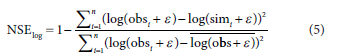
where simi, obsi and and obs are as for Eq. 1, ε is the 10th percentile of the non-zero values of observed value.
RESULTS AND DISCUSSION
Generating a precipitation grid surface
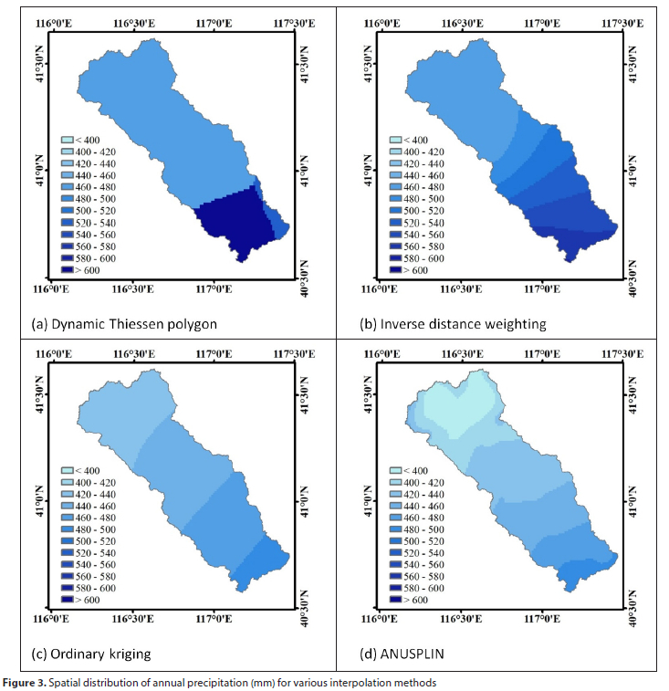
We generated the long time-series of daily precipitation interpolation surfaces using Thiessen polygon, inverse distance weighting, ordinary kriging, and ANUSPLIN interpolation methods. The precipitation time-series surface generated by the four kinds of interpolation methods showed distinct variations in distributions and quantities. We aggregated the daily precipitation time-series surfaces to annual precipitation (Fig. 3) throughout the study period (1961 to 1998). The result shows that the annual precipitation in the south is larger than it is in the north. The annual precipitation is 509.75 mm, 501.93 mm, 452.99 mm, and 434.60 mm for the Thiessen polygon, inverse distance weighting, ordinary kriging, and ANUSPLIN interpolation methods, respectively. The annual precipitation distribution from the Thiessen polygon interpolation method cannot reflect the real spatial distribution of precipitation due to the drawback of this method. The ANUSPLIN interpolation method shows more reasonable details of how precipitation is distributed in the region. The more reliable distribution information for precipitation is a benefit of this method, considering the impact of topography on precipitation in the basin.
Parameterization of the four hydrological models
The time-series data for rainfall (P), reference evapotranspiration (E) and river flow (Q) are the necessary input data for the four selected rainfall-runoff models in the Chaohe River basin. The reference evapotranspiration (E) was calculated with the Penman-Monteith formula. The time-series data for the study period (1961-1998) were divided into the calibration period (1961-1970) and validation period (1971-1998), with 1 year (365 days) for the warming up for these models. The parameters of the four model setups in this study and their ranges are shown in Table 1.
The root-mean-square error (RMSE) was selected as the objective function with suitably good optimization results for the four models (GR4J, IHACRES, Sacramento and MIKE SHE model) during the calibration and validation process. The unit for the RMSE was mm, with an optimum value of 0. The optimizing result of selecting both RMSE and NSE as the objective function is similar as both are optimizing the sum of squared residuals.
In this study, the population simplex evolution (PSE) method was selected as the optimization algorithm for the MIKE SHE model. This method is a global optimization algorithm that supports parallel optimization operations in automatic rate timing. The shuffled complex evolution (SCE) algorithm (Duan et al., 1992) was used to calibrate the parameter values for the GR4J, IHACRES and Sacramento models. The SCE algorithm is a global search algorithm that is one of the commonly used methods for parameter calibration. Research shows that the SCE algorithm is relatively efficient and can effectively optimize the hydrological models with similar results to other optimization algorithms (Shin, 2013).
Hydrologic modelling for various precipitation estimation methods
Precipitation, interpolated by Thiessen polygon, IDW, ordinary kriging and ANUSPLIN rainfall interpolation methods, was used to drive four hydrological models, GR4J, IHACRES, Sacramento and MIKE SHE. The RMSE was used as a target function to calibrate the models, and we simulated the models in the calibration period (1961-1970) and validation period (1971-1998) using the optimized parameters through calibrating in each model, to compare the precision of different precipitation interpolation methods in hydrological simulations. The NSE was selected as the evaluation index for model simulation accuracy. The daily and monthly performance of the models with different precipitation interpolation methods is shown in Tables 2 and 3.
Compared with daily NSE (Table 2), monthly NSE (Table 2) shows better performance as it is close to the optimal value, but the basic discipline for the comparison of different models and different interpolation methods is the same.
From Tables 2 and 3, the applicability of the hydrological model or rainfall interpolation method can be evaluated intuitively. Of the four hydrological models for the Chaohe River Basin, the performance of the GR4J model was worse than that of the IHACRES, Sacramento and MIKE SHE models, while that of the IHACRES, Sacramento and MIKE SHE models was similar. MIKE SHE performed more poorly when using the kriging and IDW rainfall estimates compared to IHACRES and Sacramento models (performed comparably to GR4J). Of the four precipitation interpolation methods, ANUSPLIN performed slightly better than the others. When ANUSPLIN-interpolated precipitation was used as the input for the hydrological model, the simulation accuracy of all four hydrological models was improved. The combination of the ANUSPLIN precipitation interpolation method and the Sacramento model had the highest Nash efficiency coefficient (monthly NSE = 0.88 and 0.71 for calibration and validation period). ANUSPLIN performed significantly better than the other rainfall estimation methods for the distributed model during the validation period. The daily runoff simulation results of the four models for the calibration and validation period, using the ANUSPLIN interpolation as the input, are shown in Fig. 4.
The IHACRES, Sacramento and MIKE SHE models showed good performance in modelling the high flows. The Sacramento model showed some underestimates for low flow, while the IHACRES model showed some overestimations for low flow. GR4J tended to overestimate high flows and underestimate low flows. The MIKE SHE model performed well for both high flow and low flow. The IHACRES, Sacramento and MIKE SHE models performed better than GR4J.
Uncertainty analysis of model parameters
ANUSPLIN-interpolated precipitation was used as the precipitation input to drive the hydrological models to analyse the uncertainty of hydrological model parameters. Previous experience showed that good results can be obtained when the sample size of the parameter group in the GLUE uncertainty method is large. In this study, the GLUE method was adopted by randomly selecting 100 000 group parameters to simulate. Two indicators, NSE and NSElog, were selected as the likelihood functions for uncertainty analysis for the four hydrological models (GR4J, IHACRES, Sacramento and MIKE SHE) in the Chaohe River Basin. In this paper, the modelling period was defined as 1961 to 1970 (10 years) for parameter uncertainty analysis using GLUE.
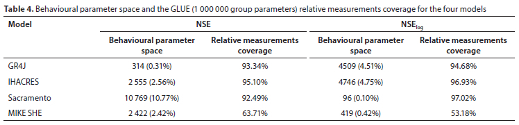
The behavioural parameter space and relative measurement coverage may be used as further criteria for the evaluation of different models. The behavioural parameter space describes the number (and percentage) of behavioural solutions (or parameters) in a given number of simulations. With the given number of parameter sets generated by the same Monte Carlo random sampling method, the behavioural parameter space is compared with the same criteria of acceptability employed (i.e., the same threshold value and the objective function) for the different models. It is also important to determine if the measurements of runoff fall within the posterior uncertainty bounds, even though the uncertainties in model predictions are considerably reduced in posterior analysis. The relative measurement coverage depicts the observed runoff covered by the uncertainty bounds. The higher behavioural parameter space means it is easier to get the behavioural parameters, and implicitly conveys the information that the model performs better. As to the comparison of relative measurement coverage for various models, a wider coverage means better performance in the modelling.
The statistics for the number of behavioural parameter sets and the 90% confidence intervals of the GLUE (1 000 000 group parameters) relative measurement coverage for four models are shown in Table 3, using a threshold value of NSE > 0.3 (or NSElog > 0.3) for the GR4J model and a threshold value of NSE > 0.5 (or NSElog > 0.5) for IHACRES, Sacramento and MIKE SHE models. The GLUE algorithm found that when NSE was selected as the objective function, there were, respectively, 314, 2 555, 10 769 and 2 422 behavioural parameter sets in 100 000 simulations for the GR4J, IHACRES, Sacramento and MIKE SHE models. When NSElog was selected as the objective function, there were respectively 4 509, 4 746, 96, and 419 behavioural parameter sets in 100 000 simulations for the GR4J, IHACRES, Sacramento and MIKE SHE models (see Table 4). For the IHACRES models, the sample acceptance rate with NSElog as the objective function was slightly higher than that with NSE as the objective function. For the GR4J models, the sample acceptance rate with NSElog as the objective function was much higher than that with NSE as the objective function. We may choose NSE or NSElog while assessing model performance for the IHACRES model, while NSElog may be better for evaluating the GR4J model. However, for the Sacramento and MIKE SHE models, the sample acceptance rate with NSElog as the objective function was less than that with NSE as the objective function. This implicitly conveys that Sacramento or MIKE SHE models perform better while using NSE as the objective function for optimizing parameters. For the GR4J, IHACRES and Sacramento models, the relative measurement coverage was slightly wider when NSElog was selected as the objective function. For the MIKE SHE model, the relative measurement coverage was wider when NSE was selected as the objective function. The evaluation indicator NSE is recommended in the hydrologic modelling of the MIKE SHE model. Overall NSE is recommended for the optimisation of hydrologic modelling in the Chaohe watershed.
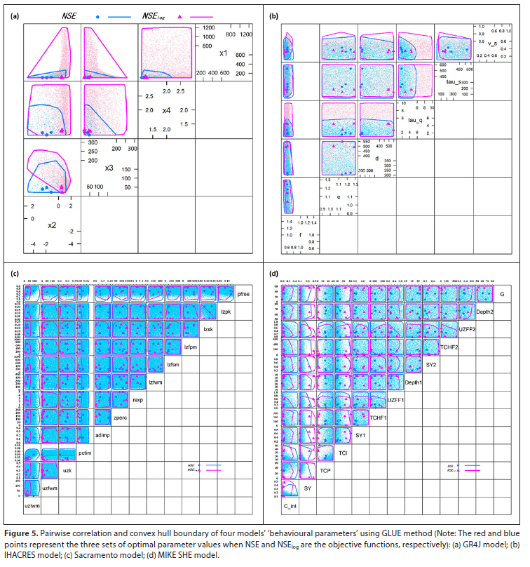
Using the pairwise correlation plot and the convex hull boundary of behaviour parameters allows simultaneous analysis of the behaviour parameters for different objective functions, which is convenient for determining accurately and effectively the distribution and sensitivity of behaviour parameters. The pairwise correlation plot and convex hull boundary of the selected parameters for the GR4J, IHACRES, Sacramento and MIKE SHE models are shown in Fig. 5. The purple (blue) dots or polygons represent behavioural parameters or the convex hull boundary of behavioural parameters for hydrologic models using NSE (NSElog) as an objective function separately.
For the GR4J model, the four parameters were highly sensitive since they yielded a small range. When NSElog was the objective function, the sensitivity of the parameter X2 (groundwater exchange coefficient) was relatively concentrated in high-value areas. When taking NSElog as the objective function, the distribution of the behaviour parameter X4 (calculation time of unit line 1) was uniform. At this point, the sensitivity of parameter X4 was low and the uncertainty was great. The sensitivity of parameter X4 was higher when NSE was the objective function.
The results of the IHACRES model showed that the sensitivity of parameters f (watershed water loss pressure threshold) and v_s (slow runoff as a percentage of total runoff) was relatively high. When NSE was chosen as the objective function, tau_q (fast runoff regression time constant) was more sensitive, while the distribution of parameters e and tau_s (slow runoff regression time constant) was more uniform, with low sensitivity and high uncertainty.
As can be seen from Fig. 5c, when NSE was taken as the objective function, the behaviour parameters of uzfwm (upper zone free water maximum capacity), uzk (upper zone free water lateral depletion rate), zperc (maximum percolation rate coefficient), rexp (exponent of the percolation equation), lzfsm (lower zone supplementary free water maximum capacity), lzfpm (lower zone primary free water maximum capacity) and lzpk (lower zone primary free water depletion rate) in the Sacramento model were uniformly distributed, and these parameters were less sensitive to high flow and had greater uncertainty. The distribution of parameter lzsk (lower zone supplementary free water depletion rate) was relatively low when NSElog was the objective function, but slightly higher when NSE was the objective function, which indicated that lzsk was sensitive to both low flow and high flow. The parameters uztwm (upper zone tension water maximum capacity) and pctim (fraction of the impervious area) were sensitive when NSElog and NSE were the objective functions, while pfree (fraction percolating from upper to lower zone free water storage) was sensitive when NSElog was the objective function.
In the MIKE SHE model, the distributions of UZFF1 (UZ feedback fraction 1), UZFF2 (UZ feedback fraction 2) and C_int (canopy interception), obtained by choosing NSElog as the objective function, were lower than those obtained with NSE as the objective function. UZFF1 and UZFF2 were related to groundwater outflow, so they were more sensitive to low flow than to high flow. The distribution of the SY (specific yield) and TCI (interflow time constant) parameters obtained by selecting NSE as the objective function was lower than that obtained using NSElog as the objective function, while the distribution of TCP (percolation time constant) was higher, indicating that the sensitivity of these three parameters to high flow may be larger than their sensitivity to low flow. The distribution of the parameters Depth1 (depth of the bottom of the reservoir 1), Depth2 (depth of the bottom of the reservoir 2) and G (bed resistance) presented a uniform distribution pattern, with low parameter sensitivity and greater uncertainty. The parameters C_int, SY and TCI were sensitive when NSElog and NSE were the objective functions, while UZFF1 and UZFF2 were sensitive when NSElog was the objective function. From the paired scatter diagram and convex hull boundary of the MIKE SHE model's behaviour parameters (Fig. 5d), a similar behaviour parameter distribution pattern could be identified. Parameters C_int, SY and TCI were sensitive when NSElog and NSE were the target functions, while UZFF1 and UZFF2 were sensitive when NSElog was the target function.
CONCLUSIONS
This study focused on the applicability of different precipitation interpolation methods in hydrological modelling. The Chaohe River Basin located in northeastern Beijing was selected as the study area. We evaluated it by comparing the performance of four different precipitation interpolation methods (Thiessen, IDW, kriging and ANUSPLIN) in the hydrological model of the Chaohe River basin. We also chose four typical hydrological models (GR4J, IHACRES, Sacramento and MIKE SHE) for this study, ranging from a lumped model to a distributed model, with simple to complex model parameters. From the different precipitation interpolation inputs, the highest precision of rainfall input was selected to drive the hydrological models. The parameter uncertainty of four hydrological models was also analysed based on uncertainty analysis from the multi-objective GLUE algorithm.
Compared to ANUSPLIN, Thiessen polygons, inverse distance weighting, and ordinary kriging were much easier to use and accessible. The ANUSPLIN needs extra topography information during the interpolation. However, the ANUSPLIN method performed better than other methods, followed by IDW and kriging, while the Thiessen polygons performed relatively poorly in the comparison of these four widely used precipitation interpolation methods. The precipitation surface generated by ANUSPLIN depicts a more reasonable distribution, which would generate better rainfall-runoff modelling in hydrologic models (including distributed model MIKE SHE). Among the four hydrological models of the Chaohe River basin, the IHACRES model, Sacramento model and MIKE SHE model performed better than the GR4J model. The ANUSPLIN precipitation interpolation surface combined with the Sacramento model gave the best result (monthly NSE = 0.88 for the calibration period and monthly NSE = 0.71 for the validation period) comprehensively.
Furthermore, the parameter sensitivity and uncertainty of the hydrologic models in the Chaohe River watershed were determined using the GLUE method. We found that the sensitivity and uncertainty of the parameters were very distinct and varied while using NSElog and NSE as the objective functions. Overall, the sensitive parameters include X2 and X4 for the GR4J model, f, v_s, and tau_q for the IHACRES model, uztwm, pctim and pfree for the Sacramento model, and C_int, SY, TCI, UZFF1 and UZFF2 for the MIKE SHE model in the Chaohe River watershed. The behavioural parameter space and the GLUE relative measurements coverage show that the NSE objective function is recommended for evaluating and optimizing hydrologic models in the Chaohe watershed.
DATA AVAILABILITY STATEMENT
Some or all data, models, or codes that support the findings of this study are available from the corresponding author upon request.
ACKNOWLEDGEMENT
This research was funded by the National Key R&D Program of China (2017YFC0406004), NSFC (41271004), the Natural Science Foundation of Hunan Province (2021JJ40012), and A Project Supported by Scientific Research Fund of Hunan Provincial Education Department (20A072).
REFERENCES
ANDREWS FT, CROKE BFW and JAKEMAN AJ (2011) An open software environment for hydrological model assessment and development. Environ. Modell. Softw. 26 (10) 1171-1185. https://doi.org/10.1016/j.envsoft.2011.04.006 [ Links ]
BEVEN KJ (1996) Equifinality and uncertainty in geomorphological modelling. In: Rhoads BL and Thorn CE (eds.), The Scientific Nature of Geomorphology. Wiley, Chichester 289-313. [ Links ]
BLASONE R, MADSEN H and ROSBJERG D (2008) Uncertainty assessment of integrated distributed hydrological models using GLUE with Markov chain Monte Carlo sampling. J. Hydrol. 353 (1-2) 18-32. https://doi.org/10.1016/j.jhydrol.2007.12.026 [ Links ]
BURNASH RJC, FERRAL RL, MCGUIRE RA, MCGUIRE RA and JOINT FRFC (1973) A Generalized Streamflow Simulation System: Conceptual Modeling for Digital Computers: U.S. Department of Commerce, National Weather Service, and State of California, Department of Water Resources. [ Links ]
CHRISTIAENS K and FEYEN J (2002) Constraining soil hydraulic parameter and output uncertainty of the distributed hydrological MIKE SHE model using the GLUE framework. Hydrol. Process. 16 (2) 373-391. https://doi.org/10.1002/hyp.335 [ Links ]
CROKE BFW, ISLAM A, GHOSH J and KHAN MA (2011) Evaluation of approaches for estimation of rainfall and the unit hydrograph. Hydraul. Res. 42 (5) 372-385. https://doi.org/10.2166/nh.2011.017 [ Links ]
DUAN Q, SOROOSHIAN S and GUPTA V (1992) Effective and efficient global optimization for conceptual rainfall-runoff models. Water Resour. Res. 28 (4) 1015-1031. https://doi.org/10.1029/91WR02985 [ Links ]
EDIJATNO, DE OLIVEIRA NASCIMENTO N, YANG X, MAKHLOUF Z and MICHEL C (1999) GR3J: a daily watershed model with three free parameters. Hydrol. Sci. J. 44 (2) 263-277. https://doi.org/10.1080/02626669909492221 [ Links ]
ESRI (2012) ArcGIS desktop: release 10.1. Environmental Systems Research Institute, Redlands, California. [ Links ]
GUO B, ZHANG J, XU T, CROKE B, JAKEMAN A, SONG Y, YANG Q, LEI X and LIAO W (2018) Applicability assessment and uncertainty analysis of multi-precipitation datasets for the simulation of hydrologic models. Water. 10 (11) 1611. https://doi.org/10.3390/w10111611 [ Links ]
HABERLANDT U (2007) Geostatistical interpolation of hourly precipitation from rain gauges and radar for a large-scale extreme rainfall event. J. Hydrol. 332 (1-2) 144-157. https://doi.org/10.1016/j.jhydrol.2006.06.028 [ Links ]
HONG Y, NIX HA, HUTCHINSON MF and BOOTH TH (2005) Spatial interpolation of monthly mean climate data for China. Int. J. Climatol. 25 (10) 1369-1379. https://doi.org/10.1002/joc.1187 [ Links ]
HUTCHINSON MF (1995) Interpolating mean rainfall using thin plate smoothing splines. Int. J. Geogr. Inf. Syst. 9 (4) 385-403. https://doi.org/10.1080/02693799508902045 [ Links ]
HUTCHINSON MF and XU T (2013) ANUSPLIN Version 4.4 User Guide. Fenner School of Environment and Society, The Australian National University, Canberra. [ Links ]
KRAUSE P, BOYLE DP and B SE F (2005) Comparison of different efficiency criteria for hydrological model assessment Adv. Geosci. 5 89-97. https://doi.org/10.5194/adgeo-5-89-2005 [ Links ]
NASH JE and SUTCLIFFE JV (1970) River flow forecasting through conceptual models part I - A discussion of principles. J. Hydrol. 10 (3) 282-290. https://doi.org/10.1016/0022-1694(70)90255-6 [ Links ]
OLIVER MA and WEBSTER R (1990) Kriging: a method of interpolation for geographical information systems. Int. J. Geogr. Inf. Syst. 4 (3) 313-332. https://doi.org/10.1080/02693799008941549 [ Links ]
OUDIN L, ANDRÉASSIAN V, MATHEVET T, PERRIN C and MICHEL C (2006) Dynamic averaging of rainfall-runoff model simulations from complementary model parameterizations. Water Resour. Res. 42 (7). https://doi.org/10.1029/2005WR004636 [ Links ]
PERRIN C, MICHEL C and ANDRÉASSIAN V (2003) Improvement of a parsimonious model for streamflow simulation. J. Hydrol. 279 (1-4) 275-289. https://doi.org/10.1016/S0022-1694(03)00225-7 [ Links ]
PHILIP GM and WATSON DF (1982) A precise method for determining contoured surfaces. APPEA J. 22 (1) 205-212. https://doi.org/10.1071/AJ81016 [ Links ]
PODGER A, SIMIC A, HALTON J, SHERGOLD P and MAHER T (2004) Integrated leadership system in the Australian Public Service (Vol. 63). https://doi.org/10.1111/j.1467-8500.2004.00407.x [ Links ]
SHIN MHS (2013) Procyclicality and the Search for Early Warning Indicators. International Monetary Fund, Washington DC. [ Links ]
SZCZEŚNIAK M and PINIEWSKI M (2015) Improvement of hydrological simulations by applying daily precipitation interpolation schemes in meso-scale catchments. Water. 7 (2) 747-779. https://doi.org/10.3390/w7020747 [ Links ]
TE CHOW V, MAIDMENT DR and MAYS LW (1988) Applied Hydrology. McGraw-Hill, New York. [ Links ]
THIESSEN AH (1911) Precipitation averages for large areas. Mon. Weather. Rev. 39 (7) 1082-1089. https://doi.org/10.1175/1520-0493(1911)39<1082b:PAFLA>2.0.CO;2 [ Links ]
TOMCZAK M (1998) Spatial interpolation and its uncertainty using automated anisotropic inverse distance weighting (IDW)-cross-validation/jackknife approach. J. Geogr. Inf. Decision Anal. 2 (2) 18-30. [ Links ]
VANSTEENKISTE T, TAVAKOLI M, NTEGEKA V, DE SMEDT F, BATELAAN O, PEREIRA F and WILLEMS P (2014) Intercomparison of hydrological model structures and calibration approaches in climate scenario impact projections. J. Hydrol. 519 743-755. https://doi.org/10.1016/j.jhydrol.2014.07.062 [ Links ]
VREBOS D, VANSTEENKISTE T, STAES J, WILLEMS P and MEIRE P (2014) Water displacement by sewer infrastructure in the Grote Nete catchment, Belgium, and its hydrological regime effects. Hydrol. Earth. Syst. Sci. 18 (3) 1119-1136. https://doi.org/10.5194/hess-18-1119-2014 [ Links ]
 Correspondence:
Jing Zhang
Email: 5607@cnu.edu.cn
Received: 5 March 2021
Accepted: 6 July 2022

