


Services on Demand
Article
 English (pdf)
 Article in xml format
 Article references
Indicators

Related links
-
 Cited by Google
 -
 Similars in Google
Share

 Permalink
Water SA
On-line version ISSN 1816-7950
Print version ISSN 0378-4738
Water SA vol.48 n.2 Pretoria Apr. 2022
http://dx.doi.org/10.17159/wsa/2022.v48.i2.3917
RESEARCH PAPER
Per capita water consumption for benchmarked South African service levels derived by means of explicit reasoning
HE JacobsI; ML CrouchI; A IlemobadeII; JL du PlessisIII
IDepartment of Civil Engineering, Stellenbosch University, Private Bag X1, Matieland 7602, South Africa
IISchool of Civil and Environmental Engineering, University of the Witwatersrand, Private Bag 3, Wits 2050, South Africa
IIIBernoulli (Pty) Ltd, 631 Rita Street, Moreletapark, Pretoria 0044, South Africa
ABSTRACT
Per capita water use is commonly employed in single-parameter models to estimate water demand, especially in regions where model input parameters are limited. Research has confirmed that the serviced population and household size positively correlate with water consumption, but the per capita consumption of household members decreases with increased household size. A central issue driving this study was the lack of an up-to-date per capita household water use guideline in the South African context. This study followed a process of explicit reasoning and inference, informed by an extensive knowledge review, stakeholder input and interrogation of relevant data, to develop a novel per capita water use estimation tool. Five main parameters were included, namely: (i) level of water service provided, (ii) usage scenario, (iii) household size (people per household), (iv) geographic region, and (v) regional property value. A Microsoft Excel-based tool was developed and is supplied online as supplementary material with this publication. The litres per capita per day tool (LCD-tool) allows for robust per capita water use estimates, as a function of the above five input parameters. The Microsoft Excel LCD-tool provides benchmarks for different South African conditions, described by context-specific service levels. The planning and management of water supply and distribution systems could benefit from the findings of this study.
Keywords: per capita water use, distribution system, planning, service levels
INTRODUCTION
Per capita water use, as a baseline estimation unit, is widely utilised for estimating water demand (DHS, 2019). This is especially true in developing regions, where the availability of additional independent variables for more complex estimation models may be limited. Despite the popularity of per capita-based estimates (e.g., DHS, 2019), research related to water use in South Africa has mainly involved plot size (also called stand size in earlier publications) as an independent variable (Jacobs et al., 2004; Van Zyl et al., 2008). A few other local studies included the independent variables of property value and household income (Husselman and Van Zyl, 2005), rainfall, temperature, evaporation and service levels (Griffioen and Van Zyl, 2014) and also water pressure (Meyer et al., 2018). A need was identified to consolidate and compare available local information regarding per capita water use and to provide unique South African benchmarks, for service levels relevant to South African conditions. The tool presented in this paper could be used for estimating per capita water consumption in the absence of recorded water use, for example, when planning water infrastructure of new housing developments in urban settings, or for setting realistic consumption targets in water demand management plans.
Objectives
The main purpose of this study was to develop a South African benchmark of per capita water use. The objectives were to: (i) conduct a knowledge review focusing on South Africa, (ii) collect relevant per capita consumption data from local studies, (iii) develop a structured approach to describe per capita water use in relation to a set of specific indicators, (iv) develop an estimation tool in MS Excel format, and (v) illustrate the typical ranges of per capita consumption experienced locally as a function of the selected input variables.
METHODOLOGY
The study involved applied research techniques. Inference and explicit reasoning were employed as deliberative operations. As part of this process, data were gathered, processed, organized, structured, and interpreted, ultimately resulting in an explicit knowledge-based tool for estimating per capita water use. Published values were collected by means of a comprehensive desktop review, supported by targeted requests to local experts and stakeholder workshops. Where household water use was available in combination with the corresponding household size, the per capita use was calculated.
Water loss and leakage are common at residential homes (Lugoma et al., 2012). Wasteful usage at standpipes is also a common phenomenon. Real water losses were not considered in this study as a water use category. Real losses could instead be estimated separately and added to the per capita use, in order to arrive at the total estimated system input volume.
Stakeholder engagement
Experts from industry, government, institutions and academia were consulted in a series of project-workshops, in order to expand the knowledge review and to provide relevant input in terms of model development. Three workshops were held, in Cape Town (25 July 2019), Midrand (10 June 2019) and Durban (7 August 2019). Information provided at each workshop was collated in the study's database. Relevant expert input was integrated with model development by successively adding complexity, with a particular focus on the general model structure and the selection of input variables. Preliminary results from the study were evaluated by stakeholders and feedback was incorporated by making adjustments to the model, in an iterative way.
Scope and limitations
Earlier per capita water use studies were identified, collated, and classified as being either micro-scale, where consumption is reported for household use downstream of a consumer meter (e.g. Meyer et al., 2021; Meyer et al., 2020; Du Plessis and Jacobs, 2018; Jacobs, 2007) or macro-scale, where consumption is reported for a city-wide scale, also including non-domestic use categories and water loss in the system (Du Plessis, 2007). With macro-scale studies, the total system input volume is typically divided by the total population served, to provide a crude estimate of per capita water use. The scope of this study was limited to micro-scale per capita household water use in South Africa. A summary of published per capita water use values is presented in Supplementary Material I.
In some instances, limited sample sizes were available for certain levels of service. Derivation of the water consumption tool was based on the best data that was available at the time, linked to explicit reasoning - it was not possible to present a statistically significant and validated model for any of the service levels, due to the limited sample size.
Water use
Household water use activities
Several water use activities are essential to health and hygiene. A lack of clean water often leads to a lack of hygiene, which can lead to diseases such as diarrhoea or other faecal-oral diseases, typhoid and skin and eye diseases. The Covid-19 pandemic was also found to impact urban water use (Kalbusch et al., 2020; Li et al., 2021), due to spread-prevention measures and changed habits (e.g., increased hand washing). Esrey et al. (1985) determined that the quantity of water used in a neighbourhood has a greater effect on the frequency of diarrhoea events than the quality of the water. However, some water use activities may not be vital to health and hygiene but may be considered 'essential' for maintaining a relatively higher standard of living (Blaine et al., 2012).
Levels of water service
Asefa et al. (2015) defined level of service as an informal contract between a utility and its customers for a certain degree of inconvenience. The service level, with regard to water utilities, describes the ease of access to water. WHO (2003) splits the levels of service into four categories defined by the travel distance (or time) to the access point of clean water and/or by number of access points: (i) no access, (ii) basic access, (iii) intermediate access and (iv) optimal access.
Service levels could also be linked to different categories of use (e.g., Willis et al., 2011), or even to the hierarchy of basic human needs (Crouch et al., 2021). Willis et al. (2011) described essential versus non-essential requirements as: (i) non-discretionary use essential for sustainable urban living e.g., in the local context this could be compared to standpipes or yard taps and (ii) discretionary use, linked to an improved standard of living.
Household size
Household size, measured as people per household (PPH), has been found to be the most significant factor affecting water consumption (Rathnayaka et al., 2017). Total household water use increases with household size. Conversely, the per capita value decreases as the household size increases, due to shared water-use activities. Consumption is also affected by the age and occupation of the members of a household (Browne et al., 2014; Mayer et al., 1999; Schleich and Hillenbrand, 2009). Age and occupation are excluded in basic estimation models, due to the relatively small impact it has on water use and the poor integrity of related input data.
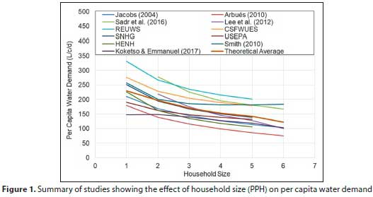
Per capita water use was found to decrease by ~22% (Schleich and Hillenbrand, 2009) and ~35% (Hõglund, 1999) with a 50% increase in household size. Numerous international empirical studies reported on measured water use for households of varying size, as graphically presented in Fig. 1 (Arbués et al., 2010; Lee et al., 2012; Sadr et al., 2016; Koketso and Emmanuel, 2017; Smith, 2010; Edwards and Martin, 1995; DeOreo and Mayer (2012); Mayer et al., 1999, USEPA Aquacraft, 2005; CSFWUES DeOreo et al., 2011).
Climatological influence
The regional climate affects water use (Van Zyl et al., 2008; Arbués, et al., 2010), with the key drivers being rainfall and temperature. The effect of climate on water use is most prominent in households with large gardens and swimming pools (Jorgensen et al., 2009). Regions with higher rainfall have lower water use than arid regions; also, the mere occurrence of rain and not necessarily the quantity of rain often reduces outdoor water use (Martinez-Espineira, 2002). Temperature also impacts use, with higher temperatures leading to increased use.
Water price, household income and property value
Household income has been correlated with water use (Ferrara, 2008; Van Zyl et al., 2008; Beal and Stewart, 2011). The law of demand states that price and demand are inversely related, with all other factors held constant. An increased price would decrease water demand and at the same time lead to an increased revenue. However, at a low price there is a limit on the amount of water anyone would use, even if it were free. On the other hand, there is a certain minimum quantity of water that anyone would require even if it were very expensive. Water price is an inconvenient parameter for inclusion in estimation models. In South Africa, the matter is complicated by free basic water allocations, non-payment, water account arrears, short-term price fluctuations brought about by seasonal water restrictions, and block tariff structures.
Household income has also been linked to water use, with higher-income families using more water in theory than similar homes with lower-income occupants (Van Zyl et al., 2008). However, reliable household income data were not readily available to use as a model input. Property value has been used as a proxy for household income before (e.g., Husselmann and Van Zyl 2006), since property value is relatively easy to obtain compared to household income.
Development of estimation tool
Various South African and international studies were reviewed in order to formulate a standardised approach that would satisfy local conditions. The tool developed as part of this project was described as the 'Litre per capita per day tool, or simply the LCD-tool. The development of the LCD-tool was purposefully aligned with other local publications, including DHS (2019). The development of the tool was also informed by expert input received during model development and at the three stakeholder workshops.
Minimum water use baseline
The departure point of model development was determination of a fundamental minimum baseline value. The minimum water requirement to meet basic health-related needs is widely accepted to be 20~25 L-c-1-d-1 (WHO 2003; Chenoweth, 2007; DHS, 2019). The minimum water use for the lowest service level in the LCD-model was set to 20 L-c-1-d-1. The value of 20 L-c-1-d-1 was considered appropriate based on input received at the project workshops, where it was pointed out that the typical container size used to carry water in many areas was reported to be ~20 L. The baseline value of 20 L-c-1-d-1 was such that the resultant water use for standpipes, with all other model inputs set to a maximum, would be 24.4 L-c-1-d-1, after application of the various multiplication factors in the model (discussed shortly). The latter aligns with 25 L-c-1-d-1 as suggested for standpipes in DWS (2019).
Level of service
The six levels of service presented by DHS (2019) were assumed to appropriately describe the South African context and were adopted in this study. Each level of service was given a sequential number by which it could be identified in the Visual Basic (VB) code:
• Standpipe (LOS1)
• Communal ablution blocks, CABs (LOS2)
• Yard connection (LOS3)
• Low-cost housing/subsidised housing (LOS4)
• Full house connection - indoor only (LOS5)
• Full house connection - including outdoor use (LOS6)
Household size
Typical household size for Western countries generally ranges between 2 and 3 PPH (House-Peters et al., 2010; Rathnayaka et al., 2017). Relatively low-income communities in developing countries, such as South Africa, have household sizes typically ranging between 5 and 10 PPH (Emenike et al., 2017; Jacobs and Haarhoff, 2004a; Mazvimavi and Mmopelwa, 2006). An upper limit of 10 PPH was considered reasonable to cover typical households in the local context. All water users on a particular property, who would be using water supplied via the consumer connection, were considered part of the 'household' for the purpose of this study - this would include backyard dwellers with access to the water supply of the main home.
Integration of household size and levels of service
A set of baseline per capita water consumption values were determined for the LCD-tool, for the range of household size and service levels. To determine the per capita consumption for each service level and each household size, all available measured South African data were compiled - focusing exclusively on measured water consumption for individual homes with known household size and level of service. Per capita consumption values based on generalised information (e.g. macro-level, census-data, or population estimates) were excluded. A summary of the measured data, showing individual plotting positions for each record, is given in Fig. 2.

The measured data were a compilation of five different datasets and classified based on the LOS. Three datasets were considered representative of LOS6, namely, a gated housing estate in Johannesburg (Ilemobade et al., 2018), 17 University of Stellenbosch student homes, and upmarket homes in Hermanus, Western Cape. Two more datasets from 20 low-cost houses in Kleinmond (Pretorius et al., 2019) and a few relatively low-income households in Eastwood, Pietermaritzburg (Smith, 2010) were considered representative of LOS4. All data that reported both the household size and water use per property, were incorporated in this study. The different datasets did not represent the same period, or geographical region, or service level. Details of each dataset can be found in the respective source document.
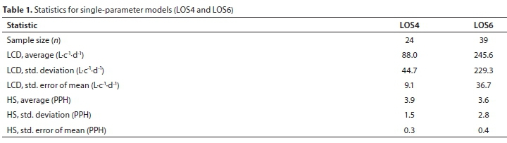
Once the data were collated, various single-parameter models were considered. Two independent models were fitted, described by Eqs 1 and 2 for LOS6 and LOS4, respectively. The relevant statistics are presented in Table 1.

where LCD = average daily per capita water consumption (L-c-1-d-1), HS = household size (PPH).
The baseline water consumption values for LOS5 were calculated as the average of LOS4 and LOS6, because no data were available for LOS5 specifically. The per capita consumption for standpipes (LOS1) was assumed to be constant over the range of household sizes - this was considered appropriate due to the fact that water is carried from the standpipe, and each additional person would typically carry another container (of fixed size) from the standpipe. No measured data were available for standpipes (linked to known per capita values) at the time of this study. Following the same reasoning as before, the values for LOS3 (yard tap) were calculated as the average of LOS1 and LOS4; LOS2 was calculated as the average of values for LOS1 and LOS3. The ultimate result, for all six service levels, is presented in Fig. 3.

Climate region
Climate has a more notable effect on households with gardens and pools (i.e., LOS6). It was considered appropriate to use a map-based input for climate, instead of adding model parameters for each relevant weather-related variable (e.g., rainfall, number of rainy days, temperature and evapotranspiration). For this purpose, maps of South African climate regions were reviewed and evaluated. The Koppen-Geiger climate classification (CSIR, 2015), based on temperature and precipitation, was selected as the most appropriate classification for the purpose of the LCD-model.
The Koppen-Geiger climate classification can be simplified as regions based on aridity. CSIR (2015) presented a map of South Africa with five aridity regions, namely: humid, moist sub-humid, dry sub-humid, semi-arid and arid. These aridity regions were used as input to the LCD-tool. The user first selects an appropriate climate region by inspecting the aridity region map (CSIR, 2015) in order to identify the region number. The relevant region number is subsequently entered as input to the LCD-model.
A factor had to be derived for the extent to which the climate region would affect water use, relative to water use in other aridity categories. Factors for high water use (arid regions) and low water use (humid regions) were first determined in relation to the average water-use values for LOS6. Jacobs et al. (2004) determined average annual water use values for increasing plot size, for four different regions of the country with varying climates, namely: Cape Town, Ekurhuleni, Windhoek and George. Even though Windhoek is not located in South Africa, the climatic factors are representative of some South African water management areas and this location was therefore considered relevant to the Koppen-Geiger classification used in this study for South Africa. Water use in Cape Town was considered to be representative of an arid region - with dry and hot summers. Windhoek and Ekurhuleni were representative of dry sub-humid regions and George was representative of relatively wet/humid regions. Subsequently, a multiplication factor of 1 was set for dry sub-humid climates, for all levels of service, with an increasing multiplication factor for increasing aridity and a decreasing multiplication factor for decreasing aridity.
In an attempt to determine the LOS6 multiplication factor for arid regions, the ratio between the water use for Windhoek and Ekurhuleni was compared to similar values for Cape Town, as presented by Jacobs et al. (2004). For a plot size of 2 000 m2, the resulting average annual water use for Windhoek and Ekurhuleni was ~1 400 L/d, while the value for Cape Town was ~1 800 L/d. The ratio of (1 800)/(1 400) suggested a multiplication factor of 1.3 for arid regions and LOS6. The multiplication factor for humid regions was based on the ratio between the water use for Windhoek and Ekurhuleni versus similar values for George. For a plot size of 2 000 m2, the average annual water use for George was ~1 000 L/d. The ratio (1 000)/(1 400) led to selection of a conservative multiplication factor of 0.75 for humid regions and LOS6. The multiplication factor for the moist sub-humid region was calculated by averaging the multiplication factors for the humid and dry sub-humid regions. The multiplication factor for the semi-arid region was calculated by averaging the multiplication factors for the arid and dry sub-humid climate regions. Climate was considered to have a minimal effect on water use for LOS1. A 10% increase and decrease in water use was assumed for LOS1 for arid and humid climates, respectively. Therefore, multiplication factors for arid and humid climates were 1.1 and 0.9. The multiplication factors for the other regions were calculated in the same manner as those for LOS6.
Water use is not linearly correlated to service level. First, the relationships between water use for each service level were determined for LOS1 and LOS6, for the humid and arid climate regions. The expected water use values, as set out by the DHS (2019), were used to determine the proportional increase in water use per service level tier. In order to interpolate the climate multiplication factors from LOS1 to LOS6, the factors were scaled in the same proportions as water use increased, per tier, from LOS1 to LOS6. The interpolation was only performed for humid and arid regions (other values were subsequently derived from these). The multiplication factors for moist sub-humid and semiarid were calculated in the same manner as that for LOS1 and LOS6, by averaging the humid and dry sub-humid and the arid and dry sub-humid conditions. A summary of all interpolated multiplication factors can be found in Table 2. For example, the unit value of 1 (for LOS1 and dry-sub humid region) would result in a water use of 20 L-c-1-d-1.
Usage level
Usage level was incorporated to compensate for relatively lower or higher water use, relative to that which was considered normal. The ratios for low and high use were adopted from other studies; for example, water use may be higher than normal due to increased outdoor use (Rathnayaka et al., 2014), low tariffs and/or non-payment, and presence of a pool (Fisher-Jeffes et al., 2015). It was considered appropriate to assume constant water use for standpipes - the volume of water serves to meet basic needs and cannot be reduced. Furthermore, since water has to be carried from the standpipe, often over long distances, excessive water use was not considered appropriate.
The usage level multiplication factor was only applied to service level tiers LOS2 to LOS6. High and low usage levels were considered to impact most notably on households with larger plot sizes. The water use for a single-person household size was used to determine the proportion between high, average and low water use. The factor derived in this manner is not independent of other inputs.
The usage level multiplication factors for LOS6 were determined first, using the theoretical household size graphs shown in Fig. 1. The average value of 240 L-c-1-d-1 was used as the departure point. The lowest and highest derived values were 179 L-c-1-d-1 and 331 L-c-1-d-1, respectively. The low water use ratio (compared to the average) for LOS6 was calculated by dividing the low water use by the average, resulting in a multiplication factor of 0.75; the resulting high water use multiplication factor was found as 1.40. All other multiplication factors were interpolated between LOS1 and LOS6 in the same manner as the multiplication factors for the humid and arid climate regions, discussed earlier. The resultant usage level multiplication factors are summarised in Table 3.
Property value
Property value was incorporated into the LCD model. Property value has been found to be positively correlated with water use (Van Zyl et al., 2008; Husselmann and Van Zyl, 2006). Specific value categories were defined so that the LCD model would find practical application in South Africa. Three property value categories were chosen, namely: (i) low-income, (ii) middle-income and (iii) high-income houses. Specific property value ranges were linked to each category and were based on available information in terms of house prices at the time of the study. Lemanski (2010) suggested a maximum value of 300 000 ZAR for a government-subsidised house in 2008. Government-subsidised housing was considered to represent the low-income portion of the population in formal housing. Considering inflation, a maximum property value of 500 000 ZAR was determined as an upper limit for low-income properties. Middle-class houses were classified with a value ranging from R 500 000 to 1 500 000 ZAR, while high-income households were classified as having a property value of greater than 1 500 000 ZAR (property values are indicative only and apply to the year 2019).
The effect of property value on water use was incorporated into the LCD-tool by adding an elasticity value, informed by earlier work (Husselmann and Van Zyl, 2006). The elasticity of water demand with respect to property value ranged between 0 and 0.5, with no clear trends reported by Husselmann and Van Zyl (2006). Considering the most basic types of service, no impact of property value on demand was assumed for standpipes, CABs and yard taps. The model was constructed with a property value elasticity that increases for the top three LOS tiers, as described below:
• Standpipes, CABs and yard connections = 0
• Low cost housing - limited in-house connections = 0.1
• Full house connection - indoor only (e.g. flats) = 0.2
• Full house connection - including outdoor = 0.3
LCD tool output
Considering the selected parameters, the tool produces a set of 270 different values (6 LOS x 3 usage scenarios x 5 regions x 3 property value categories) for each household size option.
Considering (say) 10 options of household size, for 1 to 10 PPH, the tool would produce 2 700 different results for per capita water use, depending on the selected inputs. The LCD-tool is available in MS Excel format as Supplementary Material II.
RESULTS
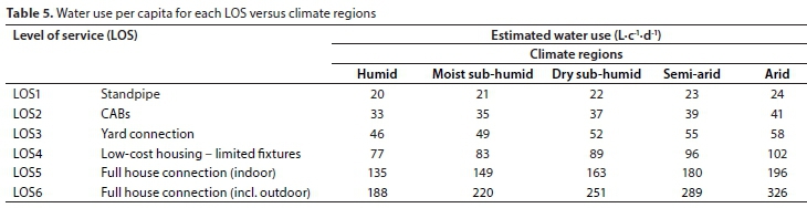
The tool was used to produce a few result sets for illustration. Two tables were created to portray the effect of changing specific parameter values. Table 4 relates to a dry sub-humid region with average water use and an average property value, with varying LOS over all tiers. The household size was varied to portray the water use for all service levels. Table 5 shows results for a 3-person household with average water use and an average property value, for each LOS. The climate region was varied in this case.
DISCUSSION
In this paper, the developed per capita water use estimation tool incorporated five parameters, namely: (i) level of water service provided, (ii) usage scenario, (iii) household size (people per household), (iv) geographic region, and (v) regional property value. Results (Tables 4 and 5) obtained from employing the estimation tool show the following:
Standpipes (LOS1), which are shared by many households and are the lowest level of service, are implemented to provide basic water supply for health and hygiene. Using the estimation tool, water use for 1 to 4 PPH was constant at 22 L-c-1-d-1 (Table 4) and varied from 20 to 24 L-c-1-d-1 (Table 5) for the different climate regions (humid to arid). In South Africa, the supply of 'Free Basic Water' (FBW), initiated by the South African Government in 2001, involves an indigent allocation, normally set at 6 kL per month per household of 8 people. The FBW quantity is therefore 25 L-c-1-d-1 and aligns with the values obtained by the estimation tool and the WHO (2003) value of ~20 L-c-1-d-1 for water collected from communal facilities.
For CABS (LOS2), estimated water use for 1 to 4 PPH varied from 54 to 34 L-c-1-d-1 (Table 4) and from 33 to 41 L-c-1-d-1 (Table 5) for the different climate regions (humid to arid). In recent years, CABs have been introduced in areas where service providers improved services to communities that were previously unserved or were dependent on yard taps. Although the arrangement of CABs varies between different suppliers and projects, they often consist of containerised showers, washbasins, laundry facilities, urinals and toilets. The Roma et al. (2010) study in Durban, South Africa, reported that CABs have a water use of between 35 and 40 L-c-1-d-1. This range aligns with the ranges obtained for CABs using the estimation tool (Tables 4 and 5).
For yard connection (LOS3), estimated water use for 1 to 4 PPH varied from 85 to 46 L-c-1-d-1 (Table 4) and from 46 to 58 L-c-1-d-1 (Table 5) for the different climate regions (humid to arid). These ranges are closely aligned to the 40 to 70 L-c-1-d-1 range suggested by Willis et al. (2011) as a set requirement for basic human needs, the DHS (2019) range of 40~80 L-c-1-d-1 for yard taps and the WHO (2003) value of ~50 L-c-1-d-1 for water collection from a single tap at each dwelling.
For LOS4, the DHS (2019) estimates water use of between 0.6 and 0.3 kL-household-1-d-1 for low-density, extra-large-sized dwellings to high-density, small-sized dwellings. These values are similar to the estimates obtained from the tool for 4 PPH (i.e., 163 L-c-1-d-1 and 76 L-c-1-d-1) from Table 4.
In this study, LOS5 (full house connection, excluding outdoor) was linked to estimates varying from 275 L-c-1-d-1 for a single-person household to 143 L-c-1-d-1 for 4 people per household. The LOS5 value could be compared to the 'realistic everyday allowable consumption level' (REAL), as described by Crouch et al. (2021). The stochastic results by Crouch et al. (2021) yielded an expected value for REAL consumption of 175 L-c-1-d-1, with a normal range of 100 L-c-1-d-1 to 251 L-c-1-d-1 for a single-person household.
For LOS6 (full house connection, including outdoor), the estimation tool estimated water use for 1 to 4 PPH ranging from 407 to 221 L-c-1-d-1 (Table 4) and from 188 to 326 L-c-1-d-1 (Table 5) for the different climate regions (humid to arid). The ratio of per capita use for LOS5:LOS6 is 275:407 (refer to Table 4) for a single-person household, or ~68%, which suggests that ~68% of the LOS6 water use could be ascribed to indoor uses. A similar ratio of 70:30 for indoor:outdoor use was reported by Meyer et al. (2021), who found that ~30% of the total annual water use in a case study of 63 residential properties in Johannesburg, South Africa, was classified as being outdoor use.
Water use of >100 L-c-1-d-1 was determined for multiple taps in a household (WHO 2003). Chenoweth (2007) noted that even though it may be theoretically feasible to meet domestic and commercial development needs with a water use of 135 L-c-1-d-1 (of which 10 - 15 L-c-1-d-1 was attributed to water loss in the system), of all currently developed countries reported on, only the United Arab Emirates and Kuwait have water use less than 135 L-c-1-d-1. Most countries reported consumption values of between 270 and 430 L-c-1-d-1, which is in line with the results from this study.
Overall, the estimation tool produces results that compare quite well with reliable water use estimates obtained for South Africa (especially the DHS, 2019) and internationally.
CONCLUSION
An extensive literature review was completed, including ~105 references to grey literature that were not specifically cited in this document. The project team obtained 63 individual data points of specific homes' per capita water use from 4 regions in the country - the most data of this nature recorded in South Africa to date. The actual data were combined with previously published literature and used as input to the model. The LCD-tool was developed in an iterative manner, amended with inputs from three workshops, held in Gauteng, Cape Town and KZN. The tool was verified by relating results to current DHS (2019) guidelines for per capita use and to international studies. The LCD-tool provides a convenient method to derive reproducible values of per capita water use, based on five different model inputs that were considered to be relatively robust and readily available.
As part of the study, a few selected key factors, namely, (i) level of service, (ii) usage scenario, (iii) the number of people per household, (iv) geographic region, (v) and property value, were incorporated in the per capita use tool. The tool was designed to be practically applicable and with a user-friendly interface in MS Excel, allowing for relatively low-cost distribution and easy access by practitioners. The tool does not account for water network losses, although on-plot losses (also called plumbing leaks) were included, because on-plot losses could not be differentiated from metered household water use.
The model outputs compared well with other studies, such as DHS (2019), although the range provided for with the LCD-tool is larger, as parameters such as climate region and number of persons per household were incorporated in this study.
ACKNOWLEDGEMENTS
This research was partly funded by the South African Water Research Commission as part of Project No. K5/2980/3.
REFERENCES
AQUACRAFT (2005) USEPA Combined retrofit report. Water and energy savings. Aquacraft Inc. and US Environmental Protection Agency, Boulder, Colorado and Washington, DC. [ Links ]
ARBUeS F, VILLANUA I and BARBERAN R (2010) Household size and residential water demand: an empirical approach. Aust. J. Agric. Resour. Econ. 54 61-80. https://doi.org/10.1111/j.1467-8489.2009.00479.x [ Links ]
ASEFA T, ADAMS A and WANAKULE N (2015) A level-of-service concept for planning future water supply projects under probabilistic demand and supply framework. J. Am. Water Resour. Assoc. 51 (5) 1272-1285. https://doi.org/10.1111/1752-1688.12309 [ Links ]
ATHURALIYA A, ROBERTS P and BROWN A (2012) Residential water use study. Yarra Valley Water, Mitcham, Australia. [ Links ]
BEAL C and STEWART A (2011) South East Queensland residential end use study: Final Report. Urban Water Security Research Alliance, Queensland. [ Links ]
BLAINE TW, CLAYTON S, ROBBINS P and GREWAL PS (2012) Homeowner attitudes and practices towards residential landscape management in Ohio, USA. Environ. Manage. 50 257-271. https://doi.org/10.1007/s00267-012-9874-x [ Links ]
BROWNE AL, PULLINGER M, MEDD W and ANDERSON B (2014) Patterns of practice: a reflection on the development of quantitative/ mixed methodologies capturing everyday life related to water consumption in the UK. Int. J. Soc. Res. Method. 17 (1) 27-43. https://doi.org/10.1080/13645579.2014.854012 [ Links ]
CHENOWETH J (2007) Minimum water requirement for social and economic development. Desalination. 229 (1-3) 245-256. [ Links ]
CROUCH ML, JACOBS HE and SPEIGHT VL (2021) Defining domestic water consumption based on personal water use activities. J. Water Suppl. Res. Technol. 70 (7) 1002-1011. https://doi.org/10.2166/aqua.2021.056 [ Links ]
CSIR (2015) Climate indicators - aridity. Regional map published by the South African Council for Scientific and Industrial Research. URL: http://stepsa.org/climate_aridity.html (Accessed 5 August 2019). [ Links ]
DEOREO WB (2011) Analysis of water use in new single family homes. Aquacraft Inc., Boulder. [ Links ]
DEOREO WB and MAYER PW (2012) Insights into declining single-family residential water demands. J. Am. Water Works Assoc. 104 (6) E383-E394. https://doi.org/10.5942/jawwa.2012.104.0080 [ Links ]
DEOREO WB, MAYER PW, MARTIEN L, HAYDEN M, FUNK A, KRAMER-DUFFIELD M and DAVIS R (2011) California single family water use efficiency study. California Department of Water Resources, Sacramento. [ Links ]
DHS (Department of Human Settlements, South Africa) (2019) The neighbourhood planning and design guide. Creating sustainable human settlements. DHS, Pretoria. [ Links ]
DIAS TF, KALBUSCH A and HENNING E (2018) Factors influencing water consumption in buildings in southern Brazil. J. Clean. Prod. 184 (20) 160-167. https://doi.org/10.1016/j.jclepro.2018.02.093 [ Links ]
DU PLESSIS JA (2007) Benchmarking water use and infrastructure based on water services development plans for nine municipalities in the Western Cape. J. S. Afr. Inst. Civ. Eng. 49 (4) 18-27. [ Links ]
DU PLESSIS JL and JACOBS HE (2018) Analysis of water use by gated communities in South Africa. Water SA. 44 (1) 130-135. http://dx.doi.org/10.4314/wsa.v44i1.15 [ Links ]
EDWARDS K and MARTIN L (1995) A methodology for surveying domestic water consumption. Water Environ. Manage. 9 (1) 447488. https://doi.org/10.1111/j.1747-6593.1995.tb01486.x [ Links ]
EMENIKE CP, TENEBE IT, OMOLE DO, NGENE BU, ONIEMAYIN BI, MAXWELL O and ONOKA BI (2017) Accessing safe drinking water in sub-Saharan Africa: Issues and challenges in South-West Nigeria. Sustainable Cities Soc. 30 263-272. https://doi.org/10.1016/j.scs.2017.01.005 [ Links ]
ESREY SA, FEACHEM RF and HUGHES JM (1985) Interventions for the control of diarrhoeal diseases among young children: improving water supplies and excreta disposal facilities. Bull. World Health Org. 63 (4) 757-772. [ Links ]
FERRARA I (2008) Residential Water Use. OECD J. General Papers. 2008 (2) 153-180. https://doi.org/10.1787/gen_papers-v2008-art14-en [ Links ]
FISHER-JEFFES L, GERTSE G and ARMITAGE NP (2015) Mitigating the impact of swimming pools on domestic water demand. Water SA. 41 (2) 238-246. https://doi.org/10.4314/wsa.v41i2.9 [ Links ]
GURAGAI B, HASHIMOTO T, OGUMA K and TAKIZAMA S (2018) Data logger-based measurement of household water consumption and micro-component analysis of an intermittent water supply system. J. Clean. Prod. 197 (1) 1159-1168. https://doi.org/10.1016/j.jclepro.2018.06.198 [ Links ]
HAY ER, RIEMANN K, VAN ZYL G and THOMPSON I (2012) Ensuring water supply for all towns and villages in the Eastern Cape and Western Cape Provinces of South Africa. Water SA. 38 (3) 437444. https://doi.org/10.4314/wsa.v38i3.9 [ Links ]
H6GLUND L (1999) Household demand for water in Sweden with implications of a potential tax on water use. Water Resour. Res. 35 3853-3863. https://doi.org/10.1029/1999WR900219 [ Links ]
HUSSELMANN ML and VAN ZYL JE (2006) Effect of stand size and income on residential water demand. J. S. Afr. Inst. Civ. Eng. 48 (3) 12-16. [ Links ]
ILEMOBADE AA, BOTHA BE and JACOBS HE (2018) Sorting high temporal resolution end-use data - a pleasurable headache. In: 1st International WDSA/CCWI 2018 Joint Conference, Kingston, Ontario, 23-25 July 2018. Paper 128, Vol. 1. [ Links ]
JACOBS HE (2007) The first reported correlation between end-use estimates of residential water demand and measured use in South Africa. Water SA. 33 (4) 549-558. [ Links ]
JACOBS HE and HAARHOFF J (2004) Application of a residential end-use model for estimating cold water and hot water demand, waste water flow and salinity. Water SA. 30 (3) 305-316. https://doi.org/10.4314/wsa.v30i3.5078 [ Links ]
JACOBS HE, GEUSTYN LC, LOUBSER BF and VAN DER MERWE B (2004) Estimating residential water demand in Southern Africa. J. S. Afr. Inst. Civ. Eng. 46 (4) 2-13. [ Links ]
JORDAN-CUEBAS F, KROGMANN U, ANDREWS CJ, SENICK JA, HEWITT EL, WENER RE, SORENSEN ALLACCI M and PLOTNIK D (2018) Understanding apartment end-use water consumption in two green residential multistory buildings. J. Water Resour. Plann. Manage. 14 (4) 1-20. https://doi.org/10.1061/(ASCE)WR.1943-5452.0000911 [ Links ]
JORGENSEN B, GRAYMORE M and O'TOOLE K (2009) Household water use behaviour: An integrated model. J. Environ. Manage. 91 227-236. https://doi.org/10.1016/j.jenvman.2009.08.009 [ Links ]
KOKETSO KN and EMMANUEL MN (2017) Water demand modelling and end-use study on households within Johannesburg, South Africa. University of the Witwatersrand, Johannesburg. [ Links ]
LEE D, PARK N and JEONG W (2012) End-use analysis of household water by metering: The case study in Korea. Water Environ. J. 26 (1) 455-464. https://doi.org/10.1111/j.1747-6593.2011.00304.x [ Links ]
LI D, ENGEL RA, MA X, PORSE E, KAPLAN JD, MARGULIS SA and LETTENMAIER DP (2021) Stay-at-home orders during the COVID-19 pandemic reduced urban water use. Environ. Sci. Technol. Lett. 2021. https://doi.org/10.1021/acs.estlett.0c00979 [ Links ]
LOH M and COGHLAN P (2003) Domestic water use study. Water Corporation, Perth. [ Links ]
LUGOMA MFT, VAN ZYL JE and ILEMOBADE AA (2012) The extent of on-site leakage in selected suburbs of Johannesburg. Water SA. 38 (1) 127-132. https://doi.org/10.4314/wsa.v38i1.15 [ Links ]
KALBUSCH A, HENNING E, BRIKALSKI MP, DE LUCA FV and KONRATH AC (2020). Impact of coronavirus (COVID-19) spread-prevention actions on urban water consumption. Resour. Conserv. Recy. 163 105098. https://doi.org/10.1016/j.resconrec.2020.105098 [ Links ]
LEMANSKI C and SAFF G (2010) The value(s) of space: The discourses and strategies of residential exclusion in Cape Town and Long Island. Urb. Affairs Rev. 45 (4) 507-543. https://doi.org/10.1177/1078087409349026 [ Links ]
MANZUNGU E and MACHIRIDZA R (2005) An analysis of water consumption and prospects for implementing water demand management at household level in the City of Harare, Zimbabwe. Phys. Chem. Earth. 30 925-934. https://doi.org/10.1016Zj.pce.2005.08.039 [ Links ]
MARTINEZ-ESPIÑEIRA R (2002) Residential water demand in the northwest of Spain. Environ. Resour. Econ. 21 (2) 161-187. https://doi.org/10.1023/A:1014547616408 [ Links ]
MAYER PW, DEOREO WB, OPITZ EM, KIEFER JC, DAVIS WY, DZIEGIELIEWSKI B and NELSON JO (1999) Residential end uses of water. AWWA Research Foundation and American Water Works Association, Denver, CO. URL: http://www.waterrf.org/PublicReportLibrary/RFR90781_1999_241A.pdf [ Links ]
MEAD N (2008) Investigation of domestic water end use. University of Southern Queensland, USQ Project. URL: https://eprints.usq.edu.au/5783/ (Deposited 1 Oct 2009). [ Links ]
MEYER BE, JACOBS HE and ILEMOBADE AI (2021) Classifying household water use into indoor and outdoor use from a rudimentary data set - A case study in Johannesburg, South Africa. J. Water Sanit. Hyg. Dev. 11 (3) 234-431. https://doi.org/10.2166/washdev.2021.229 [ Links ]
MEYER BE, JACOBS HE AND ILEMOBADE A (2020) Extracting household water use event characteristics from rudimentary data. J. Water Suppl. Res. Technol. 69 (4) 387-397. [ Links ]
MEYER N, JACOBS HE, WESTMAN T and MCKENZIE R (2018) The effect of controlled pressure adjustment in an urban water distribution system on household demand. J. Water Suppl. Res. Technol. 67 (3) 218-226. https://doi.org/10.2166/aqua.2018.139 [ Links ]
PRETORIUS D, CROUCH ML and JACOBS HE (2019) Diurnal water use patterns for low-cost houses with indigent water allocation: a South African case study. J. Water Sanit. Hyg. Dev. 9 (3) 513-521. https://doi.org/10.2166/washdev.2019.165 [ Links ]
RATHNAYAKA K, MAHEEPALA S, NAWARATHNA B, GEORGE B, MALANO H and ARORA M (2014) Factors affecting the variability of household water use in Melbourne, Australia. Resour. Conserv. Recy. 92 85-94. https://doi.org/10.1016/j.resconrec.2014.08.012 [ Links ]
RATHNAYAKA H, MALANO K, ARORA M, GEORGE B, MAHEEPALA S and NAWARATHNA B (2017) Prediction of urban residential end-use water demands by integrating known and unknown water demand drivers at multiple scales II: Model application and validation. Resour. Conserv. Recy. 118 1-12. [ Links ]
ROBERTS P (2005) Yarra Valley Water 2004 Residential End Use Measurement Study. Demand Forecasting Manager, Yarra Valley Water, Mitcham, Australia. [ Links ]
ROMA E, BUCKLEY C, JEFFERSON B and JEFFREY P (2010) Assessing users' experience of shared sanitation facilities: A case study of community ablution blocks in Durban, South Africa. Water SA. 36 (5) 589-594. https://doi.org/10.4314/wsa.v36i5.61992 [ Links ]
SADR SMK, MEMON FA, JAIN A, GULATI S, DUNCAN AP, HUSSEIN Q, SAVIC DA. and BUTLER D (2016) An analysis of domestic water consumption in Jaipur, India. Brit. J. Environ. Clim. Change. 6 (2) 97-115. https://doi.org/10.9734/BJECC/2016/23727 [ Links ]
SCHLEICH J and HILLENBRAND T (2009) Determinants of residential water demand in Germany. Ecol. Econ. 68 1756-1769. https://doi.org/10.1016/j.ecolecon.2008.11.012 [ Links ]
SHABAN A and SHARMA RN (2007) Water consumption patterns in domestic households in major cities. Econ. Polit. Weekly. 42 (23) 2190-2197. [ Links ]
SMITH JA (2010) How much water is enough? Domestic metered water consumption and free basic water volumes: The case of Eastwood, Pietermaritzburg. Water SA. 36 (5) 595-606. https://doi.org/10.4314/wsa.v36i5.61993 [ Links ]
THIEL LV (2014) Watergebruik thuis 2013. TNS Nipo, Amsterdam. [ Links ]
VAN ZYL HJ, ILEMOBADE AA and VAN ZYL JE (2008) An improved area-based guideline for domestic water demand estimation in South Africa. Water SA. 34 (3) 381-391. https://doi.org/10.4314/wsa.v34i3.180633 [ Links ]
WILLIS RM, STEWART RA, GIURCO PD, TALEBPOUR MR and MOUSAVINEJAD A (2013) End use water consumption in households: impact of socio-demographic factors and efficient devices. J. Clean. Prod. 60 107-115. https://doi.org/10.1016Zj.jclepro.2011.08.006 [ Links ]
WILLIS RM, STEWART RA, PANUWATWANICH K, WILLIAMS PR and HOLLINGSWORTH AL (2011) Quantifying the influence of environmental and water conservation attitudes on household end use water consumption. J. Environ. Manage. 92 (8) 1996-2009. https://doi.org/10.1016/j.jenvman.2011.03.023https://doi.org/10.1016/j.jenvman.2011.03.023 [ Links ]
WHO (2003) Domestic Water Quantity, Service Level and Health. World Health Organisation, Geneva. [ Links ]
 Correspondence:
HE Jacobs
Email: hejacobs@sun.ac.za
Received: 14 July 2021
Accepted: 19 April 2022

