RESEARCH PAPER

 

Utility of geospatial techniques in estimating dam water levels: insights from the Katrivier Dam

 

 

Sisipho Ngebe^I; Kasongo Benjamin Malunda^I; Anja du Plessis^II

^IDepartment of GIS and Remote Sensing, University of Fort Hare, Alice Campus, South Africa
^IIDepartment of Geography, School of Ecological and Human Sustainability, University of South Africa, Johannesburg, South Africa

Correspondence

 

 

---

ABSTRACT

To achieve informed integrated water resource management and sustainability, an understanding of the quantity of water available for use within a spatial and temporal context is needed. This study was consequently focused on the estimation of water levels with the use of geospatial techniques. The availability of water data is a significant challenge, especially for smaller dams used by farmers. The lack of consistent water data in turn poses a problem by limiting the estimation of the overall water availability in water strategy models. This challenge is attributed to the cost of modeling all available water resources and the lack of complete records of all available water resources, as some small dams are not officially registered. This paper provides a simple protocol that can be implemented to reliably derive water levels for dams that are yet to be registered or accounted for, using the Katrivier Dam as a case study. Three main datasets were used which enabled the calculation of water levels - a 12.5 m digital elevation model, Sentinel-2 optical images, and water data from the Department of Water and Sanitation (DWS), as in-situ data. The resulting water level values were derived using a proposed model that includes two correction factors, k and s. The results obtained showed that the estimated water levels from the model proposed in this paper are analogous with those observed by the DWS. Therefore, the proposed method can serve as an additional cost-effective method in water accounting procedures as it requires less expensive equipment than alternatives such as bathymetric methods.

Keywords: water level, Katrivier Dam, modified normalized difference, water index

---

 

 

INTRODUCTION

The continued increase in the world's population, as well as increasing temperatures, have placed the world's, as well as South Africa's, available freshwater resources under severe pressure through rising water demand. All relevant population dynamics and their respective water needs are placing all water resources under stress and in some cases lead to water supply problems due to low water reservoir levels. The availability of freshwater resources is changing rapidly, and in some instances has already created a fragile future, requiring major attention from scientists, policymakers and the public, especially in terms of the monitoring of water reservoirs, as these are important for managing and developing water resources for river basins regardless of their size (Liebe et al., 2005; Leemhuis et al., 2009).

Reservoir volumes are important contributors to the physical, chemical, and biological processes of water ecosystems (Lu et al., 2013). Reservoirs such as dams are the main source of water supply in many economic sectors, which primarily include, but are not limited to, agriculture, industries and municipal water use (Mustafa and Noorie, 2013). The balance between climate variables and their interactions with ecosystems, particularly between surface and groundwater, affects the state of dams and creates variability, especially in terms of its volume and total surface area (Medina et al., 2010; Lu et al., 2013).

A dam's volume and surface area are usually established through mathematical equations by relating them to depth using morphometric data (Brooks and Hayashi, 2002; Liebe et al., 2005; Gleason et al., 2007; Rodrigues et al., 2012). Water level or depth data are used as preliminary information in storage capacity models and for shallow water restoration programmes (Coops and Hosper, 2002). The variability of depth can be used as an indication of possible water quality issues as these could result in shoreline erosion during rising periods and amplify sediment depositions within a dam during receding periods, leading to imbalances in the biology of water resources due to high eutrophication and making it difficult for water managers to design appropriate countermeasures (Pasquini et al., 2008; Wildman et al., 2011). Depth is also useful in determining inter-annual and seasonal transient activities within dams (Crase and Gillespie, 2008; Garcia Molinos et al., 2015). Understanding the characteristics of a dam ensures that informed water resource management decisions are made to try to guarantee continued water security under increased anthropogenic and environmental pressures (Gamble et al., 2007; Gleason et al., 2007; Medina et al., 2010).

The most frequently used methods to calculate the physical characteristics of a dam include radar altimetry, bathymetry, echo-sounders, and global positioning systems (GPS). Bathymetry is used to measure the depth of a water body at different points, to map its surface area and underwater topography (Peng et al., 2006; Lu et al., 2013; Arsen et al., 2014). Echo-sounders estimate the depth of water bodies by sending waves through water, which is not always reliable as the velocity of the wave is greatly influenced by the chemical and physical composition of the dam under study (Annor et al., 2009). A GPS is used to collect field survey data on elevation around a water basin, together with a telescopic stadium and a rope to determine the depth of the specific water body. These methods can be used to develop surface area-volume predictive models to gain further insight into a specific water body (Liebe et al., 2005; Gleason et al., 2007; Rodrigues et al., 2012). In other cases, the depth of dams is measured utilizing in-situ gauging stations installed near river mouths, bridges, weirs, and sluices, where records of water level are obtained by systematic observations on manual recording gauges (Close et al., 2000; Sauer and Turnipseed, 2010). These gauges are limited in terms of spatial coverage and are only suitable for stable as well as less turbid rivers, lakes, and dams (Close et al., 2000; Chawira et al., 2013; Dube et al., 2014; Shumba et al., 2018).

Although developed for continental water bodies and monitoring changes in sea level, the altimetry method has been used together with satellite images to determine variations in water volumes of large lakes/reservoirs (Cretaux and Birkett, 2006; Frappart et al., 2006; Calmant et al., 2008; Gao et al., 2012; Arsen et al., 2014), to determine the slope of a river (Seyler et al., 2009), and to calculate lake water volume using the five products of radar altimetry data, namely, T/P (Topex/Poseidon), Jason-1, Jason-2, GFO (Geosat Fellow-On), ICESat, and ENVISAT (Duan and Bastiaanssen, 2013). However, the accuracy of these methods relies on the altimeter and the size of the water body (Calmant et al., 2008; Zhang et al., 2014). Regardless of the effectiveness of these methods, they have a low temporal resolution, are unable to accurately monitor steep slopes, and are expensive (Peng et al., 2006; Seyler et al., 2008; Lu et al., 2013). The development of remote sensing (RS) and geographical information systems (GIS) has addressed the overall cost issue and made it easier to evaluate the physical characteristics of reservoirs by relating depth, volume, and surface using numerical modelling, free high-resolution RS data, and RS methods that require less field work (Lu et al., 2013; Mustafa and Noori, 2013).

The study reported on in this paper used GIS and RS to estimate water levels of the Katrivier Dam through spatial model;ing. It provides a simple yet efficient method that is adaptable and cost-effective. It can be used to evaluate fluctuations in the target dam, providing detailed information about physical changes in water levels.

Literature suggests that Sentinel-2 has better characteristics than multiple other commonly accessible images, such as SPOT, Landsat, SAR, RADARSAT, and ASTER, based on spatial, temporal and spectral resolution, as well as cost (Gao et al., 2012; Rodrigues et al., 2012; Duan and Bastiaanssen, 2013; Eilander et al., 2014; Solander et al., 2016). Water index-based techniques are the most convenient methods to extract water features. These techniques are intuitive, effective and take less processing time (Ryu et al., 2002). Therefore, the modified normalized difference water index (MNDWI) has been recommended to be the best method for extracting water features (Xu, 2006; Singh et al., 2014; Dornhofer et al., 2016; Du et al., 2016; Muller et al., 2016; Kaplan and Avdan, 2017).

The Katrivier Dam was selected for this research due to it being the primary bulk water infrastructure for the whole Kat River valley. The dam supplies water to the numerous villages in the valley that lack access to potable water, and caters for an intense irrigation of commercial citrus farms, small-scale subsistence farms and livestock, as well as domestic activities. The increase in citrus farming by emerging farmers has caused an increase in water demand and has worsened the water-stressed status of the valley due to the high amount of water required for the orchards (Farolfi and Abrams, 2005; Holtzhausen, 2006). The provision of basic services will in turn increase the water requirements for domestic purposes dramatically and have a significant negative effect on the Katrivier Dam, the rural communities and small-scale farmers which depend on it for domestic purposes as well as their livelihoods, if current water use trends continue. Therefore, the valley often faces unequal access to water that weighs heavily on most farmers as well as rural communities (Mniki, 2009; Kaphayi and Celliers, 2016), insufficient supply of water leading to land degradation due to land use and land cover changes (LULC), as well as unstable climate conditions (Manyevere et al., 2014; Dube et al., 2016), and the loss of most of the distributed water due to poor local water management systems (Hay et al., 2012). A model such as the one proposed in this paper constitutes a significant contribution in the formulation of adaptable methods that can be applied locally for improved water management (Hay et al., 2012; Turpie and Visser, 2012; Donnenfield et al., 2018). This is important for farmers, especially as better accounting for water can improve water distribution mechanisms and reduce the constant conflict over water access due to water injustice that usually favors large-scale commercial famers while neglecting small-scale farmers (Kaphayi and Celliers, 2016).

Therefore, the primary aim of this paper was to develop a reliable method capable of estimating water levels and their temporal variations within the Katrivier Dam using GIS and RS, consequently obtaining and updating information regarding the characteristics of the Katrivier Dam in a more affordable manner, and ultimately expanding the water management toolbox which will be needed in the near future due to continued escalating water demands, particularly from the agricultural and domestic water use sectors.

Study area

The Katrivier Dam is located in the Kat River valley, in the Raymond Mhlaba Local Municipality (RMLM), Eastern Cape Province, South Africa (Fig. 1). The valley consists of various settlements including villages and larger urban areas. The total capacity of the dam is approximately 24.9 million m³ with a surface area of 2.129 km², and the dam's maximum water level is estimated to be 52 m. The dam is primarily used for irrigation and domestic needs (Farolfi and Abrams, 2005). Although some of the water from the dam can be accounted for through billing systems by water managers, a large part of the valley consists of rural areas accessing water for domestic use using buckets and cannot be accounted for (Turpie and Visser, 2012; Manyevere et al., 2014). Therefore, there is a need to understand the dynamics in water availability and its use. Thus, it is necessary to build a local water monitoring system that will help in understanding water variability (Turpie and Visser, 2012). This includes developing cost-effective models to monitor water availability and water usage using physical properties of the dam and its associated water dynamics.

 

METHODOLOGY

Optical satellite imagery was used to map the Katrivier Dam surface area, a digital elevation model (DEM) was used to model underwater terrain, and in-situ data was used for validation purposes.

The optical satellite Sentinel-2 is a multispectral instrument (MSI) that provides images with fine spatial resolutions of 10-, 20- and 60 m (Du et al., 2016). The satellite has a total of 13 spectral bands, with 4 (green, blue, red, and Near-infrared (NIR)) having 10 m spatial resolution, 6 (3 red-edge bands, narrow NIR, including two SWIR bands) having 20 m spatial resolution, and 3 with 60 m resolution (Drusch et al., 2012). The Sentinel-2 mission has two satellites orbiting the earth (Sentinel-2A and Sentinel-2B) and is designed to provide large coverage of land surface features and major islands around the world after each 5 days (Drusch et al., 2012).

The images downloaded were carefully selected based on the available water data provided by the DWS, to ensure that the values obtained from the proposed model were comparable to the in-situ data (Fig. 2). Thirty-two images were downloaded for dates varying from January 2019 to January 2020. It should be noted that, since the data provided by the DWS was weekly, some dates did not coincide for the satellite images and measured data. To reduce errors and bias, dates were selected to allow at most a 3-day difference between in-situ and Sentinel-2 images. Waterlevel data obtained from DWS were expressed in metres.

 

 

Therefore, a refined high-resolution Advanced Land Observing Satellite-1 (ALOS) phased array type L-band synthetic aperture radar (PALSAR) DEM, with terrain- and hydrologically corrected imagery obtained from the Alaska Satellite Facility (ASF), was used. The DEM has a spatial resolution of 12.5 x 12.5 m, and was created on 28 January 2008 on Path 599 (https://earthdata.nasa.gov/eosdis/daacs/asf).

The primary methodology followed 4 main steps: surface water mapping (SWM), underwater terrain construction (UTC), computing false water volume (CFWV), and the derivation of water levels (DWL). Thereafter, model correction coefficients (MCC) were used to adjust the derived water levels to obtain the true depth (Fig. 3).

To evaluate the accuracy of the model estimates, the root mean squared error (RMSE), the Nash-Sutcliffe efficiency (NSE), and simple linear regression (SLR) were used as validation tools, as has been applied in other studies (Lu et al., 2013; Gumindoga et al., 2018). The model was said to show a good fit if the RMSE was close to zero and the NSE close to 1. In addition, if the regression line was determined to fit the relationship y = x, then it was concluded that the data obtained from the proposed model are similar to the in-situ data, assuming x is the model and y is the in-situ data. Each method is discussed in detail in subsequent sections.

Surface water mapping

The MNDWI was used to map changes in the surface area of the Katrivier Dam. Its formula for Sentinel-2 is given as:

The MNDWI values were computed on the SNAP software using Band 3 and Band 11, setting water features to positive values while other features had negative values as soil reflects more in SWIR than in NIR light (Xu, 2006). To reduce processing time, all images were sub-set to extract only the dam extent. The resulting MNDWI were then converted into binary images separating the water body from other features. The binary images were later vectorized, to extract the water body as a surface feature.

Underwater terrain construction

To model the underwater terrain, this research used a GPS to collect elevation data. Multiple points were collected around the dam and the mean level obtained was arbitrarily selected as the overall height above sea level of the dam and estimated to be 752 m. The maximum depth (52 m) of the dam was obtained from the published data of the DWS. To reconstruct the underwater terrain, all pixels around the dam were edited by reducing the captured height by 52 m. The resulting DEM was used to build contour lines with an interval of 10 m, which were later used to create the triangulated irregular network (TIN) surface as a required standard procedure in ArcGIS under the spatial analysist extension for computing water volumes (Hollister and Milstead, 2010; Lu et al., 2013).

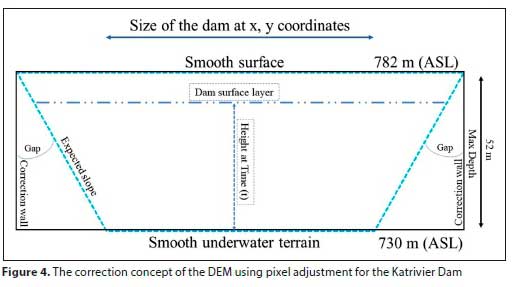
The DEM was corrected using a pixel-level adjustment; hence, three main assumptions were made in the process. The first assumption was that the dam reflecting on the DEM is the total surface area of the dam. Therefore, the adjustment was done only within those pixels outlining the dam. This resulted in the correction walls indicated in Fig. 4, instead of the expected slope. Consequently, instead of a trapezoid shape outlined by the dashed line in Fig. 4, the DEM is left with a square-like shape formed by the correction walls. This becomes a problem, given that the dam surface layer extracted from Sentinel-2 might not necessarily match the size of the dam at every x and y point on the DEM. Secondly, it was assumed that the dam was full (100%) at the time of development of the DEM. Considering that the height captured in the DEM was 782 m amsl consistently around the dam, the pixel correction process reduced the pixels around the dam to 730 m amsl. In this manner, it was then possible to set the dam surface layer obtained from Sentinel-2 at 752 m to be able to compute the false water volume in ArcGIS. Thirdly, both the surface and underwater terrain were treated as smooth topographical features. Hence, it was necessary to use correction coefficients to account for the gaps between the correction wall and the expected slope (Fig. 4).

 

 

Estimating the water level

The false water volume of the dam was calculated with the polygon volume tool in ArcMap 10.4 using the 3D Analyst toolbox (Ahmed et al., 2021). The TIN layer was used as the input surface layer, and the dam surface layers as input features set consistently at a height of 752 m, as recorded during the field survey. The obtained water volumes were then converted to metres using the proposed basin correction coefficient k = 0.1326 and a constant s = 4.5 to correct for resolution differences between input layers and account for possible gaps. Therefore, the resulting model to compute water levels became Eq. 2:

where l is the corrected water level and v the false water volume obtained from ArcGIS.

Statistical validation

Three model performance indicators were used, namely, the RMSE, the NSE, and the linear regression analysis. These indicators constitute a recommended combination for validating hydrological models (Krause et al., 2005; Hwang et al., 2012; Baloch et al., 2015; Xiaohui and Utpal, 2015).

The RMSE was computed by taking the square root of the squared sum of the residuals between the measured levels (m) and the estimated levels (e) divided by the sample size (n) (Eq. 3). The measured levels were obtained from the DWS, while the estimated levels were obtained from the proposed model.

However, the RMSE is limited in that it is highly influenced by the unit size of the datasets being compared and the lack of an agreed upon accuracy threshold, leaving the decision as to whether the errors are acceptable to the subjective assessment of the researcher. Therefore, the NSE method was used in association with the RMSE, in order to offset the limitations of the RMSE and improve on model evaluation (Xiaohui and Utpal, 2015). Based on its original design, when NSE = 1 the model matches the observed data. When NSE = 0, the model predictions are not better than the observed mean, although acceptable. However, if the NSE < 0, the model is said to be inadequate (Gumindoga et al., 2018).

The Pearson's correlation coefficient (r) and the regression parameters were used to describe the linear relationship between two variables. The two datasets were considered to be identical (follow the relationship y = x) if the intercept (β₀) is equal to zero, the slope (β₁) equal to 1, and r equal to 1 (Lu et al., 2013; Ahmed et al., 2021).

 

RESULTS AND DISCUSSION

The descriptive statistics for the datasets under investigation showed strong similarities (Table 1). The differences between the minimum, maximum, mean, and standard deviation, were below 0.7 m, whereas the median the difference was 0.8 m. The sample variances of the two datasets under analysis were closely similar, with nearly equal standard deviations, which suggests that the two samples vary similarly around the mean.

 

 

The two samples are also negatively skewed with identical range and standard error. Although the values of the in-situ data are somewhat higher than those estimated by the mo del, the expected difference between the two datasets should not be greater than a maximum of a metre in length.

While plotting the values obtained from the model compared to the ones obtained in-situ, it was determined that the largest difference in the trend was measured on 2019/10/29 at 1.31 m (red dot in Fig. 5). While most of the estimated errors were below 1 m, but within the range of 0.1-0.86 m, the minimum error was estimated at 0.03 m on 2019/01/27 and 2019/06/11 (green dots in Fig. 5).

Further analysis showed that the RMSE was 0.69 m. This suggests that, overall, there is a <1 m length difference between the two datasets. The NSE was 0.92 ~ 1, which proves that the proposed model is efficient and performs better than the observed mean as an estimator. Further evaluation, using regression analysis based on the RMSE and NSE of the predicted values, was done to determine how the proposed model performs as an estimator of storage volume. The relationship established between depth and volume from the in-situ data suggests that the two variables fit an exponential relationship better than a linear one:

If the depth obtained from the proposed model is fitted to the regression model, the RMSE of the estimated volume is 0.9 x 10⁵ m³ which, if balanced with the expected volume when depth is 0, becomes 0.3264 x 10⁵ m³ and the NSE = 0.92. These results suggest that the proposed model estimates depth within an acceptable range. Therefore, the model in its current form could also be a good predictor of water volume for the Katrivier Dam and can consequently be used as a water management tool by providing insight to enable informed decision-making.

To assess the linearity of the proposed model, the regression line was computed with β₀ initialized to zero, while observing the resulting β₁ and r. The results showed that if β₀ = 0, then β₁ = 1.018 - 1 (significant, a = 0.05), and r = 0.9969 - 1. This indicates a strong positive linear relationship between the proposed model and the in-situ data. Even though this is not a causal relationship, it does suggest that the expected variations of the two datasets are similar in at least one dimension in addition to their strong linear relationship. Therefore, both datasets could be explained in that dimension by the same variables (Fig. 6).

Therefore, it follows that the two datasets follow a relationship that can be closely expressed as y = x. This expression implies that y (the in-situ data) is not different from x (the proposed model), or at the very least, the proposed model produces accurate (similar) information about the Katrivier Dam's water level. The fact that the slope is not exactly equal to 1, implies that the proposed model will differ slightly from the in-situ data in the manner in which it estimates depth (Fig. 5). This does not however imply that the proposed model is invalid. Differences are to be expected between the estimates and the in-situ data, however minimal. Applying the regression estimates to the model showed that it is possible to reduce the differences between the proposed model and the in-situ data and improve the estimation of water levels. Therefore, Eq. 2 can be rewritten as Eq. 6:

Instead of 0.1326, k becomes 0.135, and s is adjusted to 4.581 with cL the calibrated depth. The RMSE of the embedded formula reduces to 0.23 m from the previous 0.69 m estimated using Eq. 2. The largest error was reduced to 0.30 m (red dot in Fig. 7) and the minimum error to 0 m. This shows that Eq. 6 is an improvement of Eq. 2 and displays better similarities to the DWS dataset.

Using the regression coefficient to optimize the model did however create some disadvantages. The proposed model will only be valid for the current dam and cannot be universalised, i.e., the model is context-specific. Although applying the regression coefficient improves the estimations, it is only helpful when one has in-situ data to regress the model. A better model is one that independently and reliably provides accurate data. Nevertheless, the results presented in this paper are satisfactory both before and after model calibration. Therefore, the choice of which estimate of k and s to use is left to the user if, and only if, the model is applied within the context of the Katrivier Dam. This paper focused on establishing a model specifically for this dam due to its importance, and did not engage with transferability issues of the model. The model can thus not be advocated for other dams. Furthermore, the calibrated coefficients were derived using the in-situ data, and thus may not be useful when applied to other dams.

Several issues could cause concern regarding this model and should be noted. These issues include the strength of the index used to map water features, as well as the spectral and spatial limitations of the satellite images used. Although studies have identified the MNDWI to be a better method than the NDWI or the NDVI, there is still a limit to the method's ability to differentiate certain spectral clusters such as shallow water and wet soils sharing a common boundary (Xu, 2006; Cretaux et al., 2015; Gao et al., 2012; Muller et al., 2016; Kwang et al., 2018). Therefore, one should evaluate which index better extracts water features within the context of one's research. Spatial resolution should also be considered as it can affect the accuracy when mapping spatial features in terms of their physical properties. The appropriate spatial resolution for the specific research study should also be considered when mapping specific spatial features.

Zhang et al. (2006) indicate that spatial resolution constitutes a significant influence in outlining hydrological variables presented in a DEM. This is also true for water data, especially shallow water resources (Erena et al., 2020). Thus, depending on the spatial resolution, the precision of results will vary as well. Ideally, combined images should be of the same spatial extent and spatial resolution before they can be used. Although in practice raster images will not process when combined with different extent and spatial resolution, their products can still, carefully, be used together when either one is vectorized. However, errors can still be expected when products derived from raster layers of different spatial resolutions are overlayed. Hence, within this research, correction factors were applied in an attempt to resolve these possible limitations with differences in the spatial resolutions of the input layers, which was successful based on the results obtained. Furthermore, the practice of combining images of various spatial resolutions is not new. In the majority of cases, this process is employed when the main objective is to enhance the spatial resolution of one image to match another (Wald et al., 1997; Chen et al., 2019). Therefore, to address the issue of spatial differences, images are usually fused to produce a better spatial model (Kim et al., 2020).

It is often emphasised when performing data comparisons between derivatives and measured data that all variables must be standardized in a comparable format. This also includes the temporal aspect. The information being monitored can only be validated if both the in-situ and model data are temporally in agreement (Loew et al., 2017). In the case of this paper, the data derived from the model was acquired through the use of satellite images that were captured on days that in some cases did not coincide with the dates of measurements provided by the DWS. Therefore, it is logical to assume that these temporal differences could have contributed to the differences in the estimated values. To resolve this issue, one should rely strongly on minimizing the temporal differences between the compared datasets, considering the potential of the variable under study to change over time (Loew et al., 2017). In the case of this study, changes in water levels were assumed to be minimal within the first 3 to 4 days; beyond that, and especially during dry periods, the changes become considerable and therefore may not be comparable. Hence, a limit of a 3-day difference between the date of the relevant satellite image and in-situ data was imposed in this research.

Despite the identified challenges and limitations highlighted above, there are strong merits to the proposed methods that should be emphasized and promoted. The procedure proposed in this paper ensures that the spatial and temporal resolution ofthe input variables is not significantly different to completely compromise the results. The proposed procedure further accounts for the challenges of spatial resolution differences by introducing correction coefficients that resolve this unique issue, making it possible to combine the input layers without risk of information loss. The issue of spatial differences can also be avoided if one uses input data of similar resolution, either through the acquisition of such data or through resampling. In addition, both the in-situ and Sentinel-2 images were carefully selected to minimize temporal differences. It should also be noted that the proposed model can reliably reduce estimation errors, producing data that competes with well-established entities that use sophisticated methods, without compromising on timespan or quality. The correction coefficients proposed in this paper can amend the limitations discussed earlier, consistently accounting accurately for water levels. This consequently makes the proposed model highly valuable as it is capable of providing reliable information about the depth aspect of the physical properties of a dam while smoothly resolving limitations. Hence, this method is recommended as an additional tool to frequently monitor the Katrivier Dam, due to its cost-effective implementation.

 

CONCLUSION

The research was conducted to develop a model that would be able to estimate water levels for the Katrivier Dam, through the use of no-cost protocols. Sentinel-2 data was used to map surface area variability of the dam and ALOS PALSAR's 12.5-m DEM was used to manipulate the underwater terrain of the dam. The research showed good agreement between the proposed model and in-situ data provided by the DWS. Therefore, the proposed model proved to be a possible tool to be included in the water management toolbox when attempting to calculate water levels of water bodies in a timely and cost-effective manner, which in turn can be used by water resource managers to provide guidance on water usage to domestic users and farmers, especially during periods of extended droughts. This proposed model can benefit overall water resource management within the region through the provision of accurate real-time information, enabling the equitable supply of water to all stakeholders.

The main limitations identified throughout the process of developing this proposed model included spatial resolution and atmospheric interference. However, these limitations can be minimised with appropriate correction factors. Spatial resolution limitations can be resolved; atmospheric interference then remains the only limitation which can be expected. Nevertheless, depending on the interference coverage on the obtained satellite image, this can be atmospherically corrected. Alternatively, in cases where atmospheric interferences could not be corrected, this can create missing values within the dataset, creating possible errors. In such cases, appropriate interpolation or forecasting techniques can be used to estimate the missing values. Issues of transferability of the model to other dams can be raised; cross-validation of the model is needed to ensure its fitness is not a product of pure chance. The study presented in this paper focused on the formulation of a model and did not seek to establish whether it could be standardized for all dams. This is however recommended as future research which should be undertaken to determine the cross-validity of the data. A larger dataset will however be needed to perform this cross-validation.

Save the issue of transferability, other issues such as the application of the model in terms of what it represents with respect to water usage, water safety programmes, and its implementation within existing water monitoring systems are yet to be explored. Future studies will also include the development of methods to evaluate all physical characteristics of a water body, expanding from depth to additionally estimate water volume.

Therefore, this research developed a possible model which can be adapted, with future research, to be used as a cost-effective method to monitor the variability of water resources.

 

ACKNOWLEDGMENTS

The authors acknowledge the South African National Space Agency for funding this research. In addition, acknowledgments are extended to the Department of Water and Sanitation for providing us with water level data of the Katrivier Dam, and the Copernicus data centre for the Sentinel-2 data used in this research.

 

AUTHOR CONTRIBUTIONS

Sisipho Ngebe: Responsible for writing, conception, data collection, and data analysis.

Kasongo Benjamin Malunda: Responsible for writing, conception and methodological design, data collection, data analysis, interpretation of the data and discussion of results.

Anja du Plessis: Responsible for writing, discussion of results, development of conclusions and critical revision of the paper.

 

REFERENCES

AHMED IA, SHAHFAHAD S, BAIG MRI, TALUKDAR S, ASGHER MS, USMANI TM, AHMED S and RAHMAN A (2021) Lake water volume calculation using time series LANDSAT satellite data: a geospatial analysis of Deepor Beel Lake, Guwahati. Front. Eng. Built Environ. 1 (1) 107-130 https://doi.org/10.1108/febe-02-2021-0009        [ Links ]

ANNOR FO, VAN DE GIESEN N, LIEBE J, VAN DE ZAAG P, TILMANT A and ODAI SN (2009) Delineation of small reservoirs using radar imagery in a semi-arid environment: A case paper in the upper east region of Ghana. Phys. Chem. Earth. 34 (4-5) 309-315. https://doi.org/10.1016/j.pce.2008.08.005        [ Links ]

ARSEN A, CRETAUX JF, BERGE-NGUYEN M and DEL RIO R (2014) Remote sensing-derived bathymetry of lake Poopo. Remote Sens. 6 (1) 407-420. https://doi.org/10.3390/rs6010407        [ Links ]

BALOCH MA, AMES DP and TANIK A (2015) Hydrologic impacts of climate and land-use change on Namnam Stream in Koycegiz Watershed, Turkey. Int. J. Environ. Sci. Technol. 12 (5) 1481-1494. https://doi.org/10.1007/s13762-014-0527-x        [ Links ]

BROOKS RT and HAYASHI M (2002) Depth-area-volume and hydroperiod relationships of ephemeral (vernal) forest pools in southern New England. Wetlands. 22 (2) 247-255.         [ Links ]

CALMANT S, SEYLER F and CRETAUX JF (2008) Monitoring continental surface waters by satellite altimetry. Surv. Geophys. 29 (4-5) 247-269. https://doi.org/10.1007/s10712-008-9051-1        [ Links ]

CHAWIRA M, DUBE T and GUMINDOGA W (2013) Remote sensing based water quality monitoring in Chivero and Manyame lakes of Zimbabwe. Phys. Chem. Earth. 66 38-44. http://dx.doi.org/10.1016/j.pce.2013.09.003        [ Links ]

CHEN S, WANG W and LIANG H (2019) Evaluating the effectiveness of fusing remote sensing images with significantly different spatial resolutions for thematic map production. Phys. Chem. Earth. 110 (1) 71-80. https://doi.org/10.1016Zj.pce.2018.09.002        [ Links ]

CLOSE G, LEE C, MOORE R and MOORE T (2000) Water level monitoring from space. In. Proc. International Symposium GEOMARK 2000, 10-12 April 2000, Paris, France.         [ Links ]

COOPS H and HOSPER SH (2002) Water-level management as a tool for the restoration of shallow lakes in the Netherlands. Lake Reservoir Manage. 18 (4) 293-298. https://doi.org/10.1080/07438140209353935        [ Links ]

CRASE L and GILLESPIE R (2008) The impact of water quality and water level on the recreation values of Lake Hume. Australas. J. Environ. Manage. 15 (1) 21-29. https://doi.org/10.1080/14486563.2008.9725179        [ Links ]

CRÉTAUX JF and BIRKETT C (2006) Lake studies from satellite radar altimetry. Comptes Rendus Geosci. 338 (14-15) 1098-1112. https://doi.org/10.1016/j.crte.2006.08.002        [ Links ]

CRÉTAUX JF, BIANCAMARIA S, ARSEN A, BERGÉ-NGUYEN M and BECKER M (2015) Global surveys of reservoirs and lakes from satellites and regional application to the Syrdarya river basin. Environ. Res. Lett. 10 (1). https://doi.org/10.1088/1748-9326/10/1/015002        [ Links ]

DONNENFIELD Z, CROOKES C and HEDDEN S (2018) A delicate balance: Water scarcity in South Africa. South. Afr. Rep. 13 (March) 1-24. URL: https://issafrica.org/research/southern-africa-report/a-delicate-balance-water-scarcity-in-south-africa        [ Links ]

DORNHOFER K, GORITZ A, GEGE P, PFLUG B and OPPELT N (2016) Water constituents and water depth retrieval from Sentinel-2A: A first evaluation in an oligotrophic lake. Remote Sens. 8 (11) 941. https://doi.org/10.3390/rs8110941        [ Links ]

DRUSCH M, DEL BELLO U, CARLIER S, COLIN O, FERNANDEZ V, GASCON F, HOERSCH B, ISOLA C, LABERINTI P, MARTIMORT P and MEYGRET A (2012) Sentinel-2: ESA's optical high-resolution mission for GMES operational services. Remote Sens. Environ. 120 25-36. https://doi.org/10.1016/j.rse.2011.11.026        [ Links ]

DU Y, ZHANG Y, LING F, WANG Q, LI W and LI X (2016) Water bodies' mapping from Sentinel-2 imagery with modified normalized difference water index at 10-m spatial resolution produced by sharpening the SWIR band. Remote Sens. 8 (4) 354. https://doi.org/10.3390/rs8040354        [ Links ]

DUAN Z and BASTIAANSSEN WGM (2013) Estimating water volume variations in lakes and reservoirs from four operational satellite altimetry databases and satellite imagery data. Remote Sens. Environ. 134 403-416. https://doi.org/10.1016/j.rse.2013.03.010        [ Links ]

DUBE T, GUMINDOGA W and CHAWIRA M (2014) Detection of land cover changes around Lake Mutirikwi, Zimbabwe, based on traditional remote sensing image classification techniques. Afr. J. Aquat. Sci. 39 89-95. https://doi.org/10.2989/16085914.2013.870068        [ Links ]

DUBE T, SIBANDA M and SHOKO C (2016). Examining the variability of small-reservoir water levels in semi-arid environments for integrated water management purposes, using remote sensing. Trans. R. Soc. S. Afr. 71 (1) 115-119. https://doi.org/10.1080/0035919X.2015.1102175        [ Links ]

EILANDER D, ANNOR FO, IANNINI L and VAN DE GIESEN N (2014) Remotely sensed monitoring of small reservoir dynamics: A Bayesian approach. Remote Sens. 6 (2) 1191-1210. https://doi.org/10.3390/rs6021191        [ Links ]

ERENA M, DOMÍNGUEZ JA, ATENZA JF, GARCÍA-GALIANO S, SORIA J and PÉREZ-RUZAFA A (2020) Bathymetry time series using high spatial resolution satellite images. Water. 12 (2) 1-28. https://doi.org/10.3390/w12020531        [ Links ]

FAROLFI S and ABRAMS M (2005) Water uses and their socioeconomic impact in the Kat River catchment: A report based on primary data. Report for WRC Project No. K5/1496. Water Research Commission, Pretoria.         [ Links ]

FRAPPART F, MINH KD, L'HERMITTE J, CAZENAVE A, RAMILLIEN G, LE TOAN T and MOGNARD CAMPBELL N (2006) Water volume change in the lower Mekong from satellite altimetry and imagery data. Geophys. J. Int. 167 (2) 570-584. https://doi.org/10.1111/j.1365-246x.2006.03184.x        [ Links ]

GAMBLE D, GRODY E, UNDERCOFFER J, MACK JJ and MICACCHION M (2007) An ecological and functional assessment of urban wetlands in central Ohio. Volume 2: morphometric surveys, depth-area-volume relationships, and flood storage function.         [ Links ]

Ohio EPA Technical Report WET/2007-3B. Ohio Environmental Protection Agency, Wetland Ecology Group, Division of Surface Water, Columbus.         [ Links ]

GAO H, BIRKETT C and LETTENMAIER DP (2012) Global monitoring of large reservoir storage from satellite remote sensing. Water Resour. Res. 48 (9) https://doi.org/10.1029/2012wr012063        [ Links ]

GARCIA MOLINOS J, VIANA M, BRENNAN M and DONOHUE I (2015) Importance of long-term cycles for predicting water level dynamics in natural lakes. PLoS ONE. 10 (3) e0119253. https://doi.org/10.1371/journal.pone.0119253        [ Links ]

GLEASON RA, TANGEN BA, LAUBHAN MK, KERMES KE and EULISS JR NH (2007) Estimating water storage capacity of existing and potentially restorable wetland depressions in a subbasin of the Red River of the North. Open-File Report 2007-1159. US Geological Survey, Reston, Virginia. https://doi.org/10.3133/ofr20071159        [ Links ]

GUMINDOGA W, RWASOKA DT, NCUBE N, KASEKE E and DUBE T (2018) Effect of land-cover/land-use changes on water availability in and around Ruti Dam in Nyazvidzi catchment, Zimbabwe. Water SA. 44 (1) 136-145. https://doi.org/10.4314/wsa.v44i1.16        [ Links ]

HAY ER, RIEMANN K, VAN ZYL G and THOMPSON I (2012) Ensuring water supply for all towns and villages in the Eastern Cape and Western Cape Provinces of South Africa. Water SA. 38 (3) 437-444. https://doi.org/10.4314/wsa.v38i3.9        [ Links ]

HAYASHI M and VAN DER KAMP G (2000) Simple equations to represent the volume-area-depth relations of shallow wetlands in small topographic depressions. J. Hydrol. 237 (1-2) 74-85. https://doi.org/10.1016/s0022-1694(00)00300-0        [ Links ]

HOLLISTER J and MILSTEAD WB (2010) Using GIS to estimate lake volume from limited data. Lake Reservoir Manage. 26 (3) 194-199. https://doi.org/10.1080/07438141.2010.504321        [ Links ]

HOLTZHAUSEN L (2006) Water: The tie that binds Eastern Cape community. The Water Wheel. 5 (1) 22-25.         [ Links ]

HWANG SH, HAM DH and KIM JH (2012) Une nouvelle mesure de l'efficacité des modèles hydrologiques de prévision pilotés par les données. Hydrol. Sci. J. 57 (7) 1257-1274. https://doi.org/10.1080/02626667.2012.710335        [ Links ]

KAPLAN G and AVDAN U (2017) Mapping and monitoring wetlands using sentinel-2 satellite imagery. ISPRS Annals of the Photogrammetry, Remote Sensing and Spatial Information Sciences, Volume IV-4/W4. 4^th International GeoAdvances Workshop, 14-15 October 2017, Safranbolu, Karabuk, Turkey. https://doi.org/10.5194/isprs-annals-iv-4-w4-271-2017        [ Links ]

KAPHAYI M and CELLIERS PR (2016) Factors limiting and preventing emerging farmers to progress to commercial agricultural farming in the King William's town area of the Eastern Cape province, South Africa. S. Afr. J. Agric. Ext. 44 (1) 25-41. https://doi.org/10.17159/2413-3221/2016/v44n1a374        [ Links ]

KIM Y, KYRIAKIDIS PC and PARK NW (2020) A cross-resolution, spatiotemporal geostatistical fusion model for combining satellite image time-series of different spatial and temporal resolutions. Remote Sens. 12 (10) 1553. https://doi.org/10.3390/rs12101553        [ Links ]

KRAUSE P, BOYLE DP and BASE F (2005) Comparison of different efficiency criteria for hydrological model assessment. Adv. Geosci. 5 89-97. https://doi.org/10.5194/adgeo-5-89-2005        [ Links ]

KWANG C, OSEI EM Jnr and AMOAH AS (2018) Comparing of Landsat 8 and Sentinel 2A using water extraction indexes over Volta River. J. Geogr. Geol. 10 (1) 1-7. https://doi.org/10.5539/jgg.v10n1p1        [ Links ]

LEEMHUIS C, JUNG G, KASEI R and LIEBE J (2009) The Volta Basin Water Allocation System: assessing the impact of small-scale reservoir development on the water resources of the Volta basin, West Africa. Adv. Geosci. 21. https://doi.org/10.5194/adgeo-21-57-2009        [ Links ]

LIEBE J, VAN DE GIESEN N and ANDREINI M (2005) Estimation of small reservoir storage capacities in a semi-arid environment. A case paper in the Upper East Region of Ghana. Phys. Chem. Earth. 30 448-454. https://doi.org/10.1016/j.pce.2005.06.011        [ Links ]

LOEW A, BELL W, BROCCA L, BULGIN CE, BURDANOWITZ J, CALBET X, DONNER RV, GHENT D, GRUBER A, KAMINSKI T, KINZEL J, KLEPP C, LAMBERT JC, SCHAEPMAN-STRUB G, SCHRODER M and VERHOELST T (2017) Validation practices for satellite-based Earth observation data across communities. Rev. Geophys. 55 (3) 779-817. https://doi.org/10.1002/2017RG000562        [ Links ]

LU S, OUYANG N, WU B, WEI Y and TESEMMA Z (2013) Lake water volume calculation with time series remote-sensing images. Int. J. Remote Sens. 34 (22) 7962-7973. https://doi.org/10.1080/0143116L2013.827814        [ Links ]

MANYEVERE A, MUCHAONYERWA P, LAKER M and MNKENI PNS (2014) Farmers' perspectives with regard to arable crop production and deagrarianisation: an analysis of Nkonkobe Municipality, South Africa. J. Agric. Rural Dev. Trop. Subtrop. 115 (1) 41-53.         [ Links ]

MEDINA C, GOMEZ-ENRI J, ALONSO JJ and VILLARES P (2010) Water volume variations in Lake Izabal (Guatemala) from in situ measurements and ENVISAT Radar Altimeter (RA-2) and Advanced Synthetic Aperture Radar (ASAR) data products. J. Hydrol. 382 (1-4) 34-48. https://doi.org/10.1016/j.jhydrol.2009.12.016        [ Links ]

MNIKI S (2009) Socio-economic impact of drought induced disasters on farm owners of Nkonkobe Local Municipality. Doctoral dissertation, University of the Free State.         [ Links ]

MULLER MF, YOON J, GORELICK SM, AVISSE N and TILMANT A (2016) Impact of the Syrian refugee crisis on land use and transboundary freshwater resources. In: Proc. Natl Acad. Sci. 113 (52) 14932-14937. https://doi.org/10.1073/pnas.1614342113        [ Links ]

MUSTAFA YT and NOORI MJ (2013) Satellite remote sensing and geographic information systems (GIS) to assess changes in the water level in the Duhok Dam. Int. J. Water Resour. Environ. Eng. 5 (6) 351-359.         [ Links ]

NASH JE and SUTCLIFFE JV (1970) River Flow Forecasting through Conceptual Models: Part I. A Discussion of Principles. J. Hydrol. 10 (3) 282-290.         [ Links ]

PASQUINI AI, LECOMTE KL and DEPETRIS PJ (2008) Climate change and recent water level variability in Patagonian proglacial lakes, Argentina. Glob. Planet. Change. 63 (4) 290-298. https://doi.org/10.1016/j.gloplacha.2008.07.001        [ Links ]

PENG D, GUO S, LIU P and LIU T (2006) Reservoir storage curve estimation based on remote sensing data. J. Hydrol. Eng. 11 (2) 165-172. https://doi.org/10.1061/(asce)1084-0699(2006)11:2(165)        [ Links ]

RODRIGUES LN, SANO EE, STEENHUIS TS and PASSO DP (2012) Estimation of small reservoir storage capacities with remote sensing in the Brazilian Savannah Region. Water Resour. Manage. 26 (4) 873-882. https://doi.org/10.1007/s11269-011-9941-8        [ Links ]

RYU J, WON J and MIN K (2002) Waterline extraction from Landsat TM data in a tidal flat: A case study in Gomso Bay, Korea. Remote Sens. Environ. 83 (3) 442-456. https://doi.org/10.1016/s0034-4257(02)00059-7        [ Links ]

SAUER VB and TURNIPSEED DP (2010) Stage measurement at gaging stations (p. 45). US Department of the Interior, US Geological Survey, Reston, VA.         [ Links ]

SEYLER F, CALMANT S, DA SILVA J, FILIZOLA N, COCHONNEAU G, BONNET MP and COSTI ACZ (2009) Inundation risk in large tropical basins and potential survey from radar altimetry: example in the Amazon Basin. Mar. Geodesy. 32 (3) 303-319. https://doi.org/10.1080/01490410903094809        [ Links ]

SEYLER F, CALMANT S, DA SILVA J, FILIZOLA N, ROUX E, COCHONNEAU G, VAUCHEL P and BONNET MP (2008) Monitoring water level in large trans-boundary ungauged basins with altimetry: the example of ENVISAT over the Amazon basin. Remote Sens. Inland Coast. Ocean. Waters. 7150 1-17. https://doi.org/10.1117/12.813258        [ Links ]

SHUMBA A, TOGAREPI S, GUMINDOGA W, MASARIRA T and CHIKUNI E (2018) A remote sensing and GIS based application for monitoring water levels at Kariba dam. In: EAI International Conference for Research, Innovation and Development for Africa, Kariba Gorge. p. 159. European Alliance for Innovation (EAI),. https://doi.org/10.4108/eai.20-6-2017.2270774        [ Links ]

SINGH KV, SETIA R, SAHOO S, PRASAD A and PATERIYA B (2014) Evaluation ofNDWI and MNDWI for assessment ofwaterlogging by integrating digital elevation model and groundwater level. Geocarto Int. 30 (6) 650-661. https://doi.org/10.1080/10106049.2014.965757        [ Links ]

SOLANDER KC, REAGER JT and FAMIGLIETTI JS (2016) How well will the Surface Water and Ocean Topography (SWOT) mission observe global reservoirs? Water Resour. Res. 52 (3) 2123-2140. https://doi.org/10.1002/2015wr017952        [ Links ]

TURPIE J and VISSER M (2012) The impact of climate change on South Africa's rural areas. Financial and Fiscal Commission, Midrand.         [ Links ]

WALD L, RANCHIN T and MANGOLINI M (1997) Fusion of satellite images of different spatial resolutions: Assessing the quality of resulting images. Photogramm. Eng. Remote Sens. 63 (6) 691-699.         [ Links ]

WILDMAN RA, PRATSON LF, DELEON M and HERING JG (2011) Physical, chemical, and mineralogical characteristics of a reservoir sediment delta (Lake Powell, USA) and implications for water quality during low water level. J. Environ. Qual. 40 (2) 575-586. https://doi.org/10.2134/jeq2010.0323        [ Links ]

XIAOHUI Z and UTPAL D (2015) Engaging Nash-Sutcliffe efficiency and model efficiency factor indicators in selecting and validating effective light rail system operation and maintenance cost models. J. Traffic Transport. Eng. 3 (5) 255-265. https://doi.org/10.17265/2328-2142/2015.05.001        [ Links ]

XU H (2006) Modification of normalised difference water index (NDWI) to enhance open water features in remotely sensed imagery. Int. J. Remote Sens. 27 (14) 3025-3033. https://doi.org/10.1080/01431160600589179        [ Links ]

ZHANG J, XU K, YANG Y, QI L, HAYASHI S and WATANABE M (2006) Measuring water storage fluctuations in Lake Dongting, China, by Topex/Poseidon satellite altimetry. Environ. Monit. Assess. 115 (1-3) 23-37. https://doi.org/10.1007/s10661-006-5233-9        [ Links ]

ZHANG S, GAO H and NAZ BS (2014) Monitoring reservoir storage in South Asia from multi-satellite remote sensing. Water Resour. Res. 50 (11) 8927-8943. https://doi.org/10.1002/2014wr015829        [ Links ]

 

 

Correspondence:
Kasongo Benjamin Malunda
Email: bkmalunda@gmail.com

Received: 15 March 2021
Accepted: 31 March 2022