RESEARCH PAPER

 

Flood frequency analysis - Part 1: Review of the statistical approach in South Africa

 

 

D van der Spuy; JA du Plessis

Department of Civil Engineering, Stellenbosch University, P/Bag X1, Matieland 7602, South Africa

Correspondence

 

 

---

ABSTRACT

Statistical flood frequency analyses of observed flow data are applied to develop regional empirical and deterministic design flood estimation methods, particularly for application in cases where no, or insufficient, streamflow data are available. The soundness of the statistical approach, in the estimation of flood peak frequencies, depends on the availability of long records with good-quality observed flow data. With flood frequency methods currently under review in South Africa, a sound statistical approach is considered essential. This paper reviews the statistical flood frequency approach in South Africa, which includes an appraisal of the capability of the most commonly used probability distributions in South Africa to properly cope with the challenges encountered in a flood frequency analysis, based on extended experience in flood hydrology. All the distributions tend to perform poorly when lower probability frequency events are estimated, especially where outliers are present in the dataset. Research needs are identified to improve flood peak frequency estimation techniques, and practical pointers are suggested for the interim, in anticipation of updated methods. The importance of a visual interpretation of the data is highlighted to minimise the risk of not selecting the most appropriate distribution.

Keywords: flood, frequency, exceedance, probability, distribution

---

 

 

INTRODUCTION

Different groupings of flood frequency analysis (FFA) methods, which associate a probability of exceedance, typically expressed as annual exceedance probability (AEP), with a flood peak, are reported in literature. AEP can also be expressed in terms of annual recurrence interval (ARI) or return period (T). In South Africa (SA) three classifications, commonly referred to as empirical, deterministic and statistical methods (Alexander, 1990; Pegram and Parak, 2004; Smithers, 2012; Van der Spuy and Rademeyer, 2018), are used to estimate the AEP of peak flows in an FFA.

Empirical FFA methods apply graphical or numerical relationships to translate catchment characteristics into flood peaks, deterministic methods translate catchment design rainfall into design flood peaks and hydrographs (if desired), while statistical methods are directly applied to observed flood peak data. Reference in this paper to 'statistical methods' is intended to indicate that part of statistics described as inferential statistics, in which probability theory is applied to draw conclusions from data.

The most comprehensive study on flood hydrology in SA to date was done by the Hydrological Research Unit (HRU) of the University of the Witwatersrand, at the request of the South African Institution of Civil Engineers, and their first report was published in 1969 (Midgley et al., 1969). Some of the methods proposed in this report, as well as in some of the follow-up reports (e.g. Midgley, 1972; Bauer and Midgley, 1974), were developed a few years before the first report was published, for example, an empirical method developed by Pitman and Midgley (1967). The methodologies that evolved from these studies belong to the deterministic as well as the empirical approaches and are still currently being used in SA. The deterministic and empirical methods proposed in SANRAL's Drainage Manual (SANRAL, 2013), as well as in Alexander's Flood Hydrology for Southern Africa (1990) handbook, are merely the methodologies developed by the HRU during the late 1960s.

In addition to the approaches presented in Flood Hydrology for Southern Africa (Alexander, 1990), Alexander (2002) introduced a new empirical method called the Standard Design Flood (SDF). The method generally overestimates flood magnitudes and, in several cases, even underestimates (Gericke and Du Plessis, 2012), causing some mistrust in the methodology. The latest edition of the Drainage Manual (SANRAL, 2013) also introduced the deterministic Soil Conservation Service (SCS) technique for small catchments, adapted for South African conditions (SCS-SA) by Schmidt and Schulze (1987).

Both Alexander (1990) and SANRAL (2013) include the statistical FFA for the most commonly used probability distributions in SA, namely the Log-Normal- (LN), Log-Pearson Type III- (LP3) and the General Extreme Value (GEV) distributions.

The need to develop regional methods for the estimation of design flood characteristics in ungauged basins was highlighted by Mimikou et al. (1993). Smithers (2012) also remarked that the HRU indicated that the most frequent need for design flood estimation occurs for small catchments (<15 km²). For practical and monetary reasons, most of these catchments are ungauged and observed flow and flood data do not exist. Based on various DWS FFAs (DWS,1993-2021), as also disclosed by Naidoo (2020), the deterministic and empirical approaches that were developed in SA, mainly in the 1960s, to be applied in ungauged catchments, produced results that are not consistent when compared to statistical analyses of Annual Maximum Series (AMS) flood peaks. The updating of most of these methods (Van der Spuy et al., 2004; Smithers et al., 2014) is long overdue and critical to enable an impartial assessment of the results obtained from applying the various FFA methods. More than 50 additional years of data are now available that can be utilised to improve these methods.

The South African hydrological sciences and engineering community, under the umbrella of the National Flood Studies Programme (NFSP), is currently engaged in updating or replacing deterministic and empirical design flood estimation methods in SA (Smithers et al., 2014). To realistically accomplish this, a sound statistical FFA approach will be essential.

This paper reviews the current practice relating to the statistical analysis approach in SA, based primarily on more than 27 years of practical experience gained in completing more than 850 flood frequency analyses (DWS, 1993-2021), of which just over 440 included statistical analyses. Relevant international findings are also included. Only the LN, LP3 and GEV probability distributions are considered, given their common application in SA. It is hypothesised that the issues highlighted in this paper will also be common to other approaches and probability distributions.

Hence, this paper aims to review the capability of the probability distributions most often used in SA, to properly cope with the challenges, as experienced in practice and reported in international literature, when undertaking a flood frequency analysis. Where applicable, examples are provided to highlight these challenges. The highlighted issues may inspire future research studies.

Statistical approach - the benchmark

Observed streamflow is the direct response of a catchment to a rainfall event. Consequently, a statistical analysis of streamflow data is still considered to be the most accurate 'modelling' of catchment response. Practitioners, however, still prefer to use only the deterministic and empirical methods, as opposed to a statistical analysis of flood peak data, to estimate flood frequencies. Van Vuuren et al. (2013) found that only 17% of all practitioners consider the use of statistical analyses and that only 23% of those will consider the GEV as one of the possible distributions. This was confirmed by Du Plessis (2014), with statistics of 13% and 22%, respectively.

The main reason for this seems to be the apparent lack of confidence in the statistical approaches in FFA, due to some uncertainties which mainly include, but are not limited to, the following:

• Adequate record length (Hattingh et al., 2010; Van der Spuy, 2018)

• Plotting positions with special emphasis on the plotting of 'outliers' (USACE, 1993; WMO, 2009)

• Applicability of current distributions and/or combinations thereof (NERC, 1975; Vogel et al., 1993)

• Single site vs regional analysis (Alexander, 1990; Haile, 2011; Smithers, 2012)

Practitioners also perceive that the deterministic and empirical approaches are 'easier' to apply - this perception mainly stems from the avoidance of the statistical approach.

Unfortunately, from experience gained in more than 27 years of performing numerous FFAs (DWS, 1993-2021), as well as from observations made by researchers around the world (Wallis and Wood, 1985; Gunasekara and Cunnane, 1992; Mutua, 1994; Galloway, 2010; Lettenmaier, 2010), it is evident that the current distributions do not perform very well in estimating flood peaks towards the lower AEP range, as detailed below. Low AEP flood peaks are generally overestimated, and many times grossly so, if the observed log-transformed data record yields a positive skewness coefficient.

The need for an improved, clear and reliable statistical approach is thus quite evident.

 

IMPACTS ON CHOICE OF DISTRIBUTION

Aspects that are reviewed briefly, since they can influence the choice of a distribution, include the following: (i) single site vs regional analysis approach, (ii) appropriate record length, (iii) transformation of data, (iv) the impact of outliers on the plotting position (PP), and (v) an upper bound to flood peak data.

Single site vs regional analysis

Support for the regional approach is expressed by Smithers (2012), who claims that the advantages of a regional approach for FFAs are evident from many studies (e.g. Potter, 1987; Stedinger et al., 1993; Hosking and Wallis, 1997; Cordery and Pilgrim, 2000).

Haile (2011) identified nine regions, of which five were in SA, for his study in Southern Africa. He intended to develop regional flood frequency curves, to be used in ungauged catchments, to improve the design and economic appraisal of civil engineering structures. Haile (2011) considered seven theoretical probability distributions to evaluate which will be suitable to represent the average frequency distribution of regional data. Applying probability weighted moments (PWM) and L-moments (LM) in evaluating the Generalised Pareto (GPA), GEV, Gumbel (EV1), Exponential (EXP), Three-Parameter Log-Normal (LN3), Pearson Type III (PE3) and Generalised Logistic (GLO), it was concluded that the GPA, GEV, LN3 and PE3 emerged as underlying regional distributions and that none of the three remaining distributions should be considered for regionalisation in Southern Africa.

Due to a lack of sufficient streamflow-gauging stations, regional curves could only be developed and verified for five homogeneous regions, as identified by Haile (2011), of which four are in SA. The regional curves for one of these regions are depicted in Fig. 1.

 

 

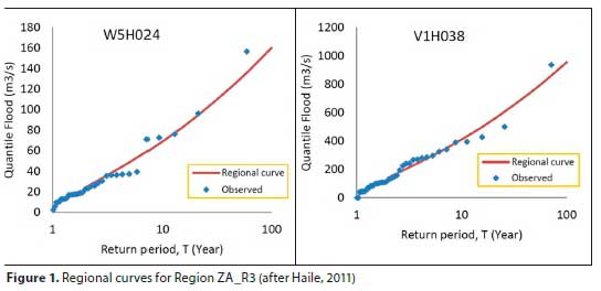
From Fig. 1 it can be concluded that outliers were clearly not adequately addressed, producing regional curves (LN3 chosen for ZA_R3) suggesting an evident absence of an upper bound for flood peaks (the outliers should not have been considered as representative of the samples, which would have changed the regional curves considerably).

Although Alexander (1990) does discuss and promote the concept of a regional analysis, the practitioner is cautioned in using it, by emphasising the need to consider the basic assumptions in this procedure, which are:

• The region within which the stations are located must be hydrologically homogeneous.

• There should be no spatial correlation between the stations used in an FFA, in a region.

Alexander (1990) also alerted the practitioner to the fact that most of the severe floods in Southern Africa are caused by widespread storms which are likely to cover most of the region. Consequently, there will nearly always be some degree of correlation between the records from the stations within the region. Alexander (2000 p. 93) reiterates his concern, stating that: "...in regional analyses the concern is the probability of floods occurring concurrently at two or more sites within a large region." Faber (2010) confirms this concern by observing that the difficulty in putting together a collection of gauged sites, independent of one another, is one of the major challenges of the regionalisation techniques. In addition, Faber (2010) commented that the large flood events tend to span multiple sites, or even an entire region, thereby causing cross-correlation between the records and consequently reducing the effective size of the dataset. This is the case in most extreme events that have occurred in SA, which raises some concerns regarding regional analyses, considering South African conditions.

Alexander (1990) also highlighted, regarding his second basic assumption above, that analytical methods for determining the grouping of stations within hydrologically homogeneous regions have indeed been developed overseas, but that these procedures required a denser network of stations than is available over most of SA, thereby indicating the need for the development of a unique approach for SA. Castellarin et al. (2012) suggested the use of the regional approach when available data record lengths are short, as compared to the AEP of interest, or for predicting the flooding potential at locations where no observed data are available.

Consequently, a regional FFA approach, for South African conditions, is deemed appropriate for the development of deterministic and empirical methods, but it is considered not to be realistic in a statistical FFA approach.

Record length

Hydrologists are repeatedly confronted with the question of when a record length is long enough to perform a sensible FFA. Hattingh et al. (2010) concluded from an investigation done in Namibia using the GEV distribution that more than 30 years of data are needed to produce consistent estimates of flood peaks in the lower AEP range.

Van der Spuy (2018) demonstrated the findings of numerous statistical analyses by presenting two typical examples with more than 100 years of streamflow data. The purpose was to highlight the minimum number of years of streamflow data needed for the distributions to produce consistent predictions in the lower AEP range. It was illustrated that the GEV distribution produced consistent results after 20 and 30 years, respectively.

In Fig. 2 the results at one of the stations are depicted. The GEV, LN and LP3 distributions, using method of moments (MM), as well as the GEV_pWM(the GEV using PWM), were fitted to the AMS. Four record lengths were considered: the observed record length of 105 years, as well as the first 20 years-, the first 40 years-and the first 70 years of the 105-year long record. The shaded areas indicate the range of results obtained for the different record lengths considered, for just the GEV and LP3, since they produced the best range of fits of the applied distributions. The Regional Maximum Flood (RMF), as an indication of the maximum expected flood for this site, is also shown (Kovacs, 1988).

 

 

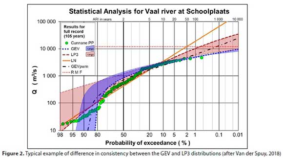
Regardless of whether 20 years, 40 years, 70 years or 105 years of annual peak flow data were used, the GEV produced results in the lower AEP range (AEP < 5% or ARI > 20 years) consistently in an exceptionally narrow band (Fig. 2).

At both representative sites presented by Van der Spuy (2018), the GEV demonstrated a higher consistency in predicting lower AEPs than the LP3, irrespective of record length, and both performed better than the LN and the GEV_PWM.

Hattingh et al. (2010) and Van der Spuy (2018) approached the problem independently and in different ways, but obtained very similar findings, admittedly using only a limited number of sites. These preliminary findings encourage further investigation into determining adequate record lengths for statistical FFA.

Transformation of data and moments

Transformation of data and/or moments primarily considers the use of log-transformed data and/or the use of different moments than MM, such as PWM or related LM. The rationale behind the transformation of data seems to be an attempt to make datasets appear more normally distributed. In doing so important statistical indicators like outliers are ignored and not properly addressed. Cunnane (1985 p. 30) confirms that proper consideration of possible outliers is avoided: "In fact low weight is given to the maximum sample value when ... parameters are estimated by maximum likelihood ... and also by probability weighted moments (PWM) ..."

Hosking et al. (1985) argued that the application of PWM outperforms the other applications in many cases and will usually be the preferred approach. Vogel et al. (1993 p. 422) used LM diagrams as a goodness-of-fit (GOF) evaluation and commented that "The GEV procedures seem to perform well for all regions considered, in spite of the fact that the L-moment diagrams do not always favour the GEV procedure." Gunasekara and Cunnane (1992), cited by Vogel et al. (1993), also confirmed the above findings. Van der Spuy (2018) reported that the GEV_PWM did not improve the results of the GEV_MM (the GEV, using MM), as is generally expected and assumed.

Wheeler (2011) advised that there is no need to transform the data to change the shape of the histogram when the data are not homogeneous, but that consideration should be given to the impact of a lack of homogeneity in the context of the original observations - for instance, in FFA, including a 1 000-year flood peak in a 50-year AMS record will indicate a lack of homogeneity, and within the context of the relative short record length will have an impact on the estimated lower AEP flood peaks.

The above sound practical advice, unfortunately, is not generally applied, which leads to the subconscious ignoring of the fact that lower AEP flood peaks may occur in a relatively short record. This results in practitioners still using various practices to transform observed data into 'more acceptable' datasets that will fit one of the current distributions (unbounded).

Plotting position and outliers

The PP are probably one of the most misunderstood and misused elements of a statistical analysis. The US Army Corps of Engineers (USACE, 1994 p. 12-5) claims that if log-transformed (flood peak) data are plotted on a log-probability grid and "if the data are truly drawn from the distribution of a log-normal parent population, the points will fall on a straight line". Hence, it might be misinterpreted by practitioners to suggest that if observed data do not fall on a straight line, the parent population cannot be a log-normal distribution, which is not necessarily correct. PPs are merely estimates of AEPs, based on ranking of observed annual maximum events. It will thus, most probably, not reflect the true AEP of observed events and it can be inferred that the PP approach will result in (i) different PPs for two or more events with the same magnitude, and (ii) a gross overestimation of the AEPs of high outliers.

The description by the WMO (2009) provides a fair explanation of the PP by identifying it as a means to provide a visual display of the data, that also serves to verify that the fitted probability distribution is consistent with the data. It is thus clearly meant as a visual check, and a quote by Watt (Posner, 2015) seems fitting here: "Do not put your faith in what statistics say, until you have carefully considered what they do not say!' All the PPs, according to the WMO (2009, citing Hirsch and Stedinger, 1987) can only provide ".crude estimates of the relative range of exceedance probabilities that could be associated with the largest events."

Although PPs are the only visual GOF check to judge the fitted probability distribution(s) against the AMS data, it is an important factor that can influence the analyst to make the wrong choice in selecting a 'best fit' distribution. For instance, Pegram and Parak (2004) suggested that the RMF had an ARI of approximately 200 years, based on the Weibull PP. Pegram and Parak (2004) then used AMS records from the three largest RMF-regions in SA at the time in their study to substantiate their claim. By their own admission they did not exclude excessively large flood peaks from the relatively short records. Thus, they did not consider that although observed outliers (as well as the RMF) will be part of the population they are not part of the relatively small AMS sample hydrologists must use to estimate what the underlying population should look like. By including these outliers in their FFAs and PPs, lower AEP flood peaks were grossly overestimated, leading to their conclusion that: ".the return period of the RMF is approximately 200 years." (p. 387). In contrast, Van der Spuy (2018) illustrated that the ARI of the RMF seems to vary between 10 000 years and 100 000 years.

This debatable conclusion comes from the misperceptions surrounding the PP, as touched on in the discussion above, especially where outliers are present in the dataset. This is evident in Fig. 3, where the different PPs are compared with each other.

 

 

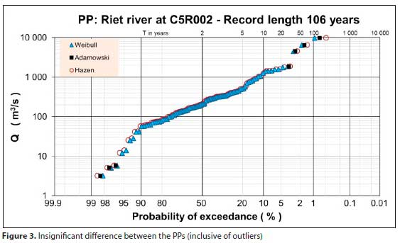
The Weibull and Hazen PPs are shown, being the two extremes, with the Adamowski PP in between. The rest of the commonly used PPs, like the Cunnane, Gringorten and Blom PPs, lie between the Adamowski and the Hazen plot (PPs from Adamowski, 1981).

It is evident from the case study presented in Fig. 3 that:

• The three highest flood peaks do not seem to be consistent with the perceptible distribution of the rest of the annual flood peak dataset.

• The claims by the developers of the PPs, namely that different PPs suit different distributions, are nonsensical. For all practical purposes they provide identical visual checks.

Recent international status of plotting positions

De Haan (2007) commented that much research has been conducted on statistical methods for extremes and that the PP is irrelevant to modern extreme value statistics. These statistical approaches include, but are not limited to, using PWM/ LM, measures of accuracy (AM) methods and GOF tests. These tests are used to test the degree of correlation between the observed data (the sample) and the distribution of expected values (the population).

Given the background of economics, the comments from De Haan (2007) might be reasonably valid, but the practice of ignoring the PP, regrettably, is also noted in some flood hydrology studies (e.g. Xiong et al., 2018; Langat et al., 2019; Ul Hassen et al., 2019; Zhang et al., 2019). 'Regrettably', because in FFA no population of AMS flood peaks exists against which the observed data records can be assessed, while the PP provides the only visual data display against which the fitted distribution can be checked.

The obvious question is: 'against what reference (population) are the AM- and GOF tests performed?' It can be argued that a 'population' of flood peaks can be stochastically generated from the observed record. However, if a 10 000-year flood occurs in a 50-year AMS record it must be considered as an outlier, in relation to the sample, not the population. Therefore, if the outlier is not excluded from the record in determining the moments to stochastically generate a population, the outlier will inherently remain at an AEP of around 2% within the population - in effect, just replicating the assigned PP probabilities.

Many freely available software packages perform GOF tests for a range of distributions. The risk of reducing an FFA to a 'black-box' exercise is real, which is a serious concern, since it takes the scientific/engineering inference and sound judgement away from the analyst. The authors therefore accept the valuable contribution of PP in the process of selecting an appropriate distribution in FFA, as still being applied in SA, and propose the continued use of it in practice.

PPs in their existing format, as an approach to check the selection of appropriate and most applicable distributions, seemingly provide a realistic trend of the middle quantiles of the underlying distribution. Although it provides a visual indication of probable outliers, it still fails to provide a more realistic PP for it (as evident in Fig. 3 and also Fig. 4). Thus, a review of the estimation of PPs, with specific attention to outliers, is required, to provide an improved informative visual tool for FFAs.

 

 

An upper bound to flood peak data

The most popular distribution functions used in FFA typically have two to four parameters with the common feature of having no upper bound. This is particularly true of log-transformed flood peak data portraying a positive skewness coefficient. Information about upper bounded (and/or lower bounded) distributions applicable to FFA are not commonly available.

Botero and Francés (2010) interrogate the practice of accepting unbounded distributions, by stating that the estimated annual maximum flood peaks in the lower AEP range increase without any limit as the AEPs decrease, in the case of unbounded probability distributions. They argue that, considering the specific characteristics of a catchment of interest, like catchment area and geomorphologic characteristics, the obvious question to ask is whether it is possible that a flood peak, with no restriction on its magnitude, can occur. Their own unequivocal response to this question was: "The straight answer is no, this is not possible" (p. 2 618).

In their study, Botero and Francés (2010) defined relative short series, recorded systematically at a flow-gauging station, as 'systematic' information, with historical and palaeoflood information as 'non-systematic' information. A site on the Jucar River in Spain with a 'systematic' AMS of 56 years and 4 'non-systematic' observed floods, dating back to 1778-1864, were used as a case study. Botero and Francés (2010) chose the Four-Parameter Extreme Value (EV4) distribution and included an estimated Probable Maximum Flood (PMF) value, to generate a flood peak record of 450 years using Monte Carlo simulations.

The EV4, the Four-Parameter Log-Normal (LN4) and the Transformed Extreme Value (TEV) distribution were applied to the data as 'upper-bounded' distributions. They used the EV4-, GEV- and the Two-Component Extreme Value (TCEV) distributions, in their robustness analyses.

Botero and Francés (2010) cited the GPA and GEV as commonly used distribution functions in hydrology which have an upper bound. The GPA is not generally used in SA in FFA and the validity of it being an upper-bound distribution is thus unknown. The GEV indeed imitates an upper-bound distribution, if plotted on a log-probability scale - when plotted on a normal-probability scale, it is obvious that the GEV is not a true upper-bound distribution.

The statement by Botero and Francés (2010), that extreme FFA should have an upper-bound, presents the potential for research into a proper upper-bound distribution. Their inference that the TCEV should not be used for estimating very low AEP flood peaks and that the GEV should only be used for high AEPs, in an upper bounded population, should be noted in future studies. Bardsley (2016) recognised that an upper bound should exist and suggested the introduction of a sufficiently high upper truncation point to the flood distribution, with a subsequent modified ARI-scale. For example, he suggested that if a 10 000-year ARI is considered as a truncation point, the ARI-scale must be adjusted to instead indicate the 10 000-year ARI as infinity (°°).

Once the concept of an upper-bound to a distribution is accepted, the impact on the associated aspects, discussed above under 'General aspects impacting on the choice of distribution' (record length, transformation of data, PPs, etc.), will have to be reconsidered.

 

APPRAISAL OF COMMONLY USED DISTRIBUTIONS

International preferences

It is important to acknowledge that there is still, in flood hydrology, disagreement on which distribution provides the 'best' fit to observed flood peak data. Despite numerous studies, three distributions seem to have withstood the test of time, namely the Log-Normal (LN), the Log-Pearson Type III (LP3) and the General Extreme Value (GEV), which consists of a family of three extreme value continuous probability distributions, with some variations in application (for example, applying different moments, using two or three parameters, etc.).

In general, the LP3 is the preferred distribution in the USA (Faber, 2010; England et al., 2018), although the use of more distributions is encouraged if the distribution of choice "... does not provide a reasonable fit to the data" (USACE, 1993 p. 3-1). In research, to identify the preferred statistical distribution for at-site FFA in Canada, Zhang et al. (2019) concluded that the GEV performs better than the other considered distributions.

In the UK the GEV distribution was preferred according to NERC (1975), which was replaced by new national guidelines in the Flood Estimation Handbook (FEH). Robson and Reed (1999) as well as Asikoglu (2018), citing Salinas et al. (2014), indicated that the GLO replaced the GEV as the preferred distribution in the UK. Castellarin et al. (2012) confirmed that several countries in Europe recommend the GEV as one of their choices, with a variety of other distributions, such as the GPA, LN, LN3, which are also used. In Australia the GPA, GEV, LN3, LP3 and the Two-Parameter Log-Normal (LN2), are considered as acceptable alternative distributions (Vogel et al., 1993). Rahman et al. (2013) confirmed that the LP3, GEV and GPA distributions have been identified as the top three best-fit flood distributions in Australia.

However, in SA the LN, LP3 and GEV, either with MM or PWM, are proposed (Alexander, 1990). Both LP3 and GEV distributions provided good results (DWS, 1993-2021) and the practice is to apply both and use the one that seems to fit the data best.

Considering the LN distribution

The normal distribution was first developed by De Moivre in 1753 (Van der Spuy and Rademeyer, 2018). The distribution is widely used in meteorology and hydrology, as well as in other civil engineering applications, such as measurement errors (survey).

Hazen (1913) is credited with having observed that while hydrological data are usually strongly skewed, the logarithms of the data have a near symmetrical distribution (Van der Spuy and Rademeyer, 2018). The LN distribution, which is a normal distribution fitted to the logarithms of the observed values, is thus also used in analysing flood peak data.

This distribution is symmetrical about the mean and is therefore only suitable for data where the skewness coefficient (g) of the log-transformed data is equal to or close to zero. If g = 0, the LP3 distribution represents the LN distribution.

Considering the LP3 distribution

In Pakistan the results of an FFA on the river Swat indicated that the LP3 and GEV ranked as the top two distributions at all four sites along the river, with LP3 the top distribution at two of the four sites (Farooq et al., 2018). In Kenya it was observed that the Wakeby and LN3 distributions outperformed all the other methods (Mutua, 1994). However, due to the complexity of the Wakeby distribution, it was suggested that the LN3 be considered as the best model for FFA in Kenya. Mutua (1994 p. 243) stated that: "One of the worst fitting distributions is found to be the three-parameter log Pearson distribution, despite its popularity within the country."

Wallis and Wood (1985 p. 1 049), also cited in Alexander (1990), indicated that the flood quantile estimates obtained from the LP3 distribution are "significantly worse" than those obtained from the GEV and Wakeby. They further commented that the US Water Resources Council (USWRC) Bulletin 17B guideline needs re-evaluation. Twenty-five years later Lettenmaier (2010 p. 269) remarked that it is time to "give Bulletin 17B a decent burial" and to move on. Galloway (2010 p. 274) simultaneously stressed that there is no time to waste and voiced the need for scientists to proceed forward with good science and to look differently at solutions, and added: "Don't help people do wrong things more precisely."

Experience has (DWS, 1993-2021) also revealed that the LP3 distribution is not only sensitive to high outliers, but can be seriously affected by low outliers, as will be discussed in the section titled 'Sensitivity of distributions to outliers'.

Considering the GEV distribution

The GEV is an extreme value distribution, seemingly less affected by lower outliers than the LP3 distribution. It will produce (generally) more reliable estimates at the lower AEPs; i.e. AEPs < 20% (ARI > 5 years). The downside, however, is that the GEV does not necessarily produce reliable estimates for AEPs > 50% (ARI < 1 in 2 years) as illustrated in Fig. 2.

Vogel et al. (1993) found that the GPA and GEV approaches are preferred in Australia outside the winter-dominated rainfall regimes and that both are also considered to probably provide the best description of flood flows across the entire Australia.

As shown in Fig. 2 and the accompanying discussion, the GEV outperforms, in general, the other distributions in SA.

Sensitivity of distributions to outliers

FFAs performed at various sites (DWS, 1993-2021) have shown that outliers will affect how probability distributions fit the observed data. MM was used, since PWM and LM tend to assign equal weight to all data points, thereby considering an outlier as part of the sample. Two of these analyses were chosen to illustrate the impact of outliers on various distributions (see Figs 4 and 5).

 

 

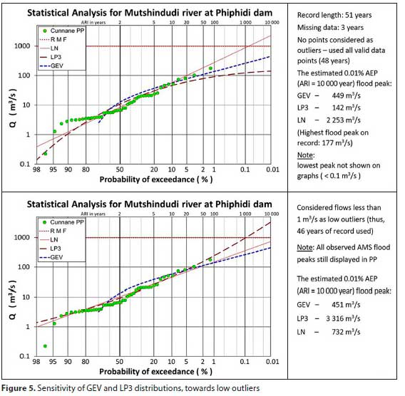
Note: In the events where the outliers are excluded, the datapoints are still displayed in the PP-plots since these remain proper observations. Hence, where it is stated that the outliers are excluded, they are only omitted in estimating the moments for the FFA.

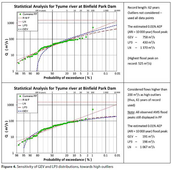
In Fig. 4, the sensitivity of the distributions to high outliers is illustrated.

The inclusion of the outlier, or not, clearly seems to have a slightly bigger effect on the GEV than on the LP3 distribution. The effect on the LN distribution was much less.

However, what is more interesting is that the exclusion of the outlier seems to have an adverse effect on both the GEV and the LP3 - to the extent that both distributions seem to deem this flood peak as not being part of the fitted distribution (no associated frequency).

In Fig. 5, the sensitivity of the distributions to lower outliers is illustrated.

In this case the inclusion of the low outlier, or not, seems to have virtually no effect on the GEV, but the LN and particularly the LP3 are adversely affected. It was observed in informal studies and numerous FFAs (DWS, 1993-2021) that the way in which the lower peaks are distributed can also affect the LP3 and LN, but the effect on the GEV is negligible.

It is thus concluded that the GEV appears to be markedly less impacted by low outliers in forecasting lower AEP flood peaks (higher ARI flood peaks) than the other two distributions, in 100% of observed cases. Conversely, all of the distributions are affected by high outliers. If high outliers are present, either the GEV or the LP3 might be impacted more than the other, but there is no clear indication of the impelling cause(s) - more research is needed.

Performance of distributions with long records

How the different distributions might perform with very long records will only be truthfully answered in the distant future, as truly long records become available.

However, to get some insight, a 100+ year observed record was used to stochastically generate a 10 000-year flow record (independently, using Monte Carlo simulation techniques) and the highest annual flood peaks were extracted from this generated record. The results, as an example, are presented in Fig. 6.

 

 

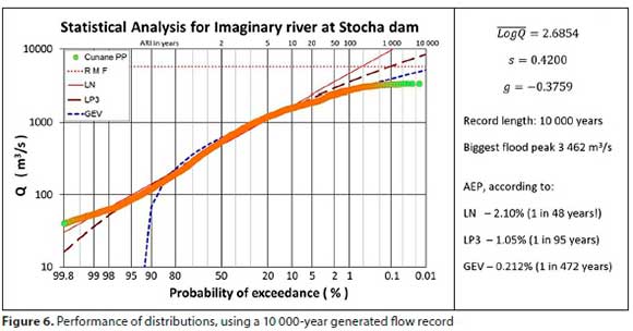
The GEV outperformed the other two distributions, in estimating lower AEP flood peaks, by a large margin (as expected), but it nonetheless 'only' assigned an AEP of 0.212%, to the highest flood peak in a 10 000-year record.

This case study supported the hypothesis that the distributions are more likely to overestimate estimated flood peaks at the lower AEPs, but the degree of overestimation with such a long record (albeit generated) was not expected.

Reflections on appraisal of distributions

Concerning current national and international practices, the above observations, used to illustrate observations from DWS (1993-2021), trigger the following questions/remarks:

• If the LN already mimics an exponential mathematical trend, should the LP3 (for example) even be considered if the log-transformed data indicate a positive skewness?

• It may, practically, be more sensible to use combinations of distributions; for example:

- Fitted distributions can be 'linked':

For example, in Fig. 5 with the outlier included, accept the LN distribution for AEPs higher than 14% and the GEV distribution for AEPs equal to or lower than 14%.

- Consequently, distributions can be 'combined' by means of weighted averages:

Both Van der Spuy (2018) and Gericke and Du Plessis (2012) concluded that an option to use combinations of multiple probability distributions can add value to finding a realistic flood peak, especially in the lower AEP domain. Gericke and Du Plessis (2012) used the Mean Logarithm Value Approach (MLVA) to illustrate the success thereof in overcoming limitations, like short record lengths, associated with the single-site approach.

For example, in Fig. 5 with the outlier excluded, accept the LN for AEPs higher than 60% and the MLVA of all three distributions for AEPs equal to or lower than 60%.

Although the above approaches will, visually, produce more pleasing fits to the plotted data, it is realised that this will probably receive criticism and serious opposition from statisticians, but who can justly claim that the best distribution for a particular dataset is not the average of two (or more) known distributions, if by omitting one or two outliers from a dataset the forecasted 10 000-year flood peak can change (using the same distribution) by more than 2 300% (LP3, Fig. 5)?

 

CONCLUSION

The purpose of this paper was to critically assess the performance of the theoretical probability distributions generally used for statistical FFA in SA.

The results indicate that none of the probability distributions seems to fit long records, especially ultra-long stochastically generated records, very well - most probably because none of the distributions has an upper bound. This paper, therefore, highlights the need to further investigate the use of a combination of probability distributions and/or a bounded probability distribution which will provide a more acceptable flood prediction estimator.

Proposed interim practical approach

There is currently no consensus amongst hydrologists, worldwide, about flood frequency methods and related issues. It seems fitting to repeat the remark made by Galloway (2010 p. 274) when he appealed to scientists to proceed forward with good science and to look differently at solutions and added: "Don't help people do wrong things more precisely."

Nonetheless, the GEV seems to be more stable than the LP3 or LN in predicting lower AEPs, irrespective of record length. The GEV also seems to be less sensitive to outliers than the LP3.

Therefore, until further research provides a more acceptable approach, from experience illustrated in this review, it is proposed that the following practical pointers be considered in SA, in an interim approach:

• Consider all three probability distributions, commonly in use in SA, namely the GEV, LP3 and LN.

• If the log-transformed data prove to have a positive skewness, the LP3 should not be considered in the lower AEP range.

• Visually compare the GOF between the various distributions and the observed annual flood peak data.

• Carefully consider all contributing factors before choosing a distribution, especially if a single distribution seems to fit all data points well, or if it is the preference of the analyst to use only a single distribution.

• It is clear from all the illustrative examples presented that, although the LP3 might be a consideration in some cases, the GEV is generally a preferred choice at the lower probabilities. However, it performs poorly above an AEP of 50%. It is thus proposed, for the interim, to consider combining it with the higher AEP results of one of the other distributions - ensuring that there is a smooth transition from the one to the other.

• A combination of distributions (e.g. the MLVA), as suggested by Van der Spuy (2018) and Gericke and Du Plessis (2012), may also be considered, to obtain more realistic flood peaks.

PPs were identified as the main challenge to deal with in an FFA, especially where outliers are present in the AMS. PPs should be re-investigated and improved to again be considered as an essential aid to the flood frequency analyst.

 

REFERENCES

ADAMOWSKI K (1981) Plotting formula for flood frequency. Water Resour. Assoc. 17 (2) 197-202. https://doi.org/10.1111/j.1752-1688.1981.tb03922.x        [ Links ]

ALEXANDER WJR (1990) Flood Hydrology for Southern Africa. South African National Committee on Large Dams, 1990.         [ Links ]

ALEXANDER WJR (2000) Flood risk reduction measures. Department of Civil Engineering, University of Pretoria, South Africa.         [ Links ]

ALEXANDER WJR (2002b) The Standard Design Flood: technical paper. J. S. Afr. Inst. Civ. Eng. 44 (1) 26-30.         [ Links ]

ASIKOGLU OL (2018) Parent flood frequency distribution of Turkish Rivers. Pol. J. Environ. Stud. 27 (2) 529-539. https://doi.org/10.15244/pjoes/75963        [ Links ]

BARDSLEY E (2016) Note on a modified return period scale for upper-truncated unbounded flood distributions. J. Hydrol. 544 452-455. https://doi.org/10.1016/j.jhydrol.2016.11.050        [ Links ]

BAUER SW and MIDGLEY DC (1974) A simple procedure for synthesising Direct Runoff Hydrograph. HRU Report 1/74. Department of Civil Engineering, University of the Witwatersrand, Johannesburg.         [ Links ]

BOTERO BA and FRANCÉS F (2010) Estimation of high return period flood quantiles using additional non-systematic information with upper bounded statistical models. Hydrol. Earth Syst. Sci. 14 26172628. https://doi.org/10.5194/hess-14-2617-2010        [ Links ]

CASTELLARIN A, KOHNOVA S, GAÁL L, FLEIG A, SALINAS JL, TOUMAZIS A, KJELDSEN TR and MACDONALD N (2012) Review of Applied-Statistical Methods for Flood-Frequency Analysis in Europe. NERC/Centre for Ecology & Hydrology. 122 pp. (ESSEM COST Action ES0901).         [ Links ]

CORDERY I and PILGRIM DH (2000) The state of the art of flood prediction. In: Parker DJ (ed.) Floods. Volume II. Routledge, London. 185 -197.         [ Links ]

CUNNANE C (1985) Factors affecting choice of distribution for flood series. Hydrol. Sci. J. 30 (1) 25-36. https://doi.org/10.1080/02626668509490969        [ Links ]

DE HAAN L (2007) Comments on "Plotting Positions in Extreme Value Analysis". J. Appl. Meteorol. Climatol. 46 (3) 396. https://doi.org/10.1175/JAM2471.1        [ Links ]

DU PLESSIS JA (2014) Unpublished results of a frequency analysis survey. Short Course on Flood Hydrology, August 2014, University of Stellenbosch.         [ Links ]

DWS (1993-2021) Flood frequency analyses intended for dam safety evaluation (numerous reports) Department of Water and Sanitation, Pretoria.         [ Links ]

ENGLAND JF (Jr), COHN TA, FABER BA, STEDINGER JR, THOMAS WO (Jr), VEILLEUX AG, KIANG JE and MASON RR (Jr) (2018) Guidelines for determining flood flow frequency. Bulletin 17C (ver. 1.1, May 2019). U.S. Geological Survey Techniques and Methods, book 4, chap. B5 148 pp. https://doi.org/10.3133/tm4B5        [ Links ]

FABER B (2010) Current methods for flood frequency analysis. In: Workshop on Non-Stationarity, Hydrologic Frequency Analysis and Water Management, 13-15 January 2010, Boulder, Colorado. 33-38. URL: https://mountainscholar.org/handle/10217/69250        [ Links ]

FAROOQ M, SHAFIQUE M and KHATTAK MS (2018) Flood frequency analysis of river Swat using Log Pearson type 3, Generalized Extreme Value, Normal, and Gumbel Max distribution methods. Arab. J. Geosci. 11 (9) 216. https://doi.org/10.1007/s12517-018-3553-z        [ Links ]

GALLOWAY GE (2010) If stationarity is dead, what do we do now? In: Workshop on Non-Stationarity, Hydrologic Frequency Analysis and Water Management, 13-15 January 2010, Boulder, Colorado. 274-280. URL: https://mountainscholar.org/handle/10217/69250        [ Links ]

GERICKE OJ and DU PLESSIS JA (2012) Evaluation of the standard design flood method in selected basins in South Africa. J. S. Afr. Inst. Civ. Eng. 54 (2) 2-14.         [ Links ]

GUNASEKARA TAG and CUNNANE C (1992) Split sampling technique for selecting a flood frequency analysis procedure. J. Hydrol. 130 (1) 189-200. https://doi.org/10.1016/0022-1694(92)90110-H        [ Links ]

HAILE AT (2011) Regional flood frequency analysis in Southern Africa. Unpublished Masters thesis, University of Oslo.         [ Links ]

HATTINGH L, CLOETE G, MOSTERT A and MUIR C (2010) The impact of hydrology on the adequacy of existing dams to safety standards - the Namibian experience. In: Proceedings of the 2^nd International Congress on Dam Maintenance and Rehabilitation, 23-25 November 2010, Zaragoza, Spain.         [ Links ]

HAZEN A (1913) Storage to be provided in impounding reservoirs for municipal water supply. Proc. Am. Soc. Civ. Eng. 39 (9) 1943-2044.         [ Links ]

HIRSCH RM and STEDINGER JR (1987) Plotting positions for historical floods and their precision. Water Resour. Res. 23 (4) 715727. https://doi.org/10.1029/WR023i004p00715        [ Links ]

HOSKING JRM and WALLIS JR (1997) Regional Frequency Analysis: An Approach Based on L-Moments. Cambridge University Press, Cambridge 224 pp.         [ Links ]

HOSKING JRM, WALLIS JR and WOOD EF (1985) Estimation of the generalized extreme-value distribution by the method of probability-weighted moments. Technometrics. 27 (3) 251-261. https://doi.org/10.2307/1269706        [ Links ]

KOVACS Z (1988) Regional maximum flood peaks in Southern Africa. Technical Report 137. Department of Water Affairs, South Africa.         [ Links ]

LANGAT PK, KUMAR L and KOECH R (2019) Identification of the most suitable probability distribution models for maximum, minimum, and mean streamflow. Water. 11 (4) 734. https://doi.org/10.3390/w11040734        [ Links ]

LETTENMAIER D (2010) Workshop Summary I. In: Workshop on Non-Stationarity, Hydrologic Frequency Analysis and Water Management, 13-15 January 2010, Boulder, Colorado. 268-273. https://mountainscholar.org/handle/10217/69250        [ Links ]

MIDGLEY DC (1972) Design flood determination in South Africa.         [ Links ]

HRU Report No. 1/72. Department of Civil Engineering, University of the Witwatersrand, Johannesburg.         [ Links ]

MIDGLEY DC, PULLEN RA and PITMAN WV (1969) Design flood determination in South Africa. HRU Report No. 4/69. Department of Civil Engineering, University of the Witwatersrand, Johannesburg.         [ Links ]

MIMIKOU M, NIADAS P, HADJISSAVA P and KOUVOPOULOS Y (1993) Regional prediction of extreme design storm and flood characteristics. Water Power & Dam Construction, December 1993.         [ Links ]

MUTUA FM (1994) The use of the Akaike Information Criterion in the identification of an optimum flood frequency model. Hydrol. Sci. J. 39 (3) 235-244. https://doi.org/10.1080/02626669409492740        [ Links ]

NAIDOO J (2020) An assessment of the performance of deterministic and empirical design flood estimation methods in South Africa. Unpublished Masters thesis. University of KwaZulu-Natal, South Africa.         [ Links ]

NERC (Natural Environment Research Council) (1975) Hydrological Studies, Vol. I, Flood Studies Report. Natural Environment Research Council, London, UK.         [ Links ]

PEGRAM G and PARAK M (2004) A review of the regional maximum flood and rational formula using geomorphological information and observed floods. Water SA. 30 (3) 377-392.         [ Links ]

PITMAN WV and MIDGLEY DC (1967) Flood studies in South Africa: frequency analysis of peak discharges. Die Siviele Ingenieur. 9 (8) 193-200.         [ Links ]

POSNER MA (2015) Michael A. Posner's page of statistics quotes. URL: http://www.posnersmith.net/quotes_s.html (Accessed 12 October 2015).         [ Links ]

POTTER KW (1987) Research on flood frequency analysis: 19831986. Rev. Geophys. 25 (2) 113-118. https://doi.org/10.1029/RG025i002p00113        [ Links ]

RAHMAN AS, RAHMAN A, ZAMAN MA, HADDAD K, AHSAN A and IMTEAZ M (2013) A study on selection of probability distributions for at-site flood frequency analysis in Australia. Nat. Hazards. 69 (3) 1803-1813. https://doi.org/10.1007/s11069-013-0775-y        [ Links ]

ROBSON AJ and REED DW (1999) Statistical Procedures for Flood Frequency Estimation. Volume 3 of the Flood Estimation Handbook. Centre for Ecology & Hydrology, Wallingford, Oxfordshire, UK.         [ Links ]

SALINAS JL, CASTELLARIN A, VIGLIONE A, KOHNOVA S and KJELDSEN TR (2014) Regional parent flood frequency distributions in Europe - Part 1: Is the GEV model suitable as a pan-European parent? Hydrology and Earth System Sciences. 18 (11) 4381-4389. https://doi.org/10.5194/hess-18-4381-2014        [ Links ]

SANRAL (South African National Roads Agency) (2013) Drainage Manual (6^th edn). South African National Roads Agency Ltd, Pretoria.         [ Links ]

SCHMIDT EJ and SCHULZE RE (1987) Flood volume and peak discharge from small catchments in Southern Africa based on the SCS technique. ACRU Report No. 24 (WRC Report No. TT 31/8). Department of Agricultural Engineering, University of Natal, Pietermaritzburg. 164 pp.         [ Links ]

SMITHERS JC (2012) Methods for design flood estimation in South Africa. Water SA. 38 (4) 633-646. https://doi.org/10.4314/wsa.v38i4.19        [ Links ]

SMITHERS JC, GORGENS A, GERICKE J, JONKER V and ROBERTS CPR (2014) The initiation of a national flood studies programme for South Africa. In: Proceedings of the SANCOLD National Conference, 5-7 November 2014, Johannesburg.         [ Links ]

STEDINGER JR, VOGEL RM and FOUFOULA-GEORGIOU E (1993) Frequency analysis of extreme events. In: Handbook of Hydrology. 18. McGraw-Hill, New York, USA.         [ Links ]

UL HASSEN M, HAYAT O and NOREEN Z (2019) Selecting the best probability distribution for atsite food frequency analysis; a study of Torne River. SN Appl. Sci. 1 1629. https://doi.org/10.1007/s42452-019-1584-z        [ Links ]

USACE (U.S. ARMY CORPS OF ENGINEERS) (1993) Engineering and Design: Hydrologic Frequency Analysis. Department of the Army, USACE EM1110-2-1415.         [ Links ]

USACE (U.S. ARMY CORPS OF ENGINEERS) (1994) Engineering and Design: Flood-Runoff Analysis. Department of the Army, USACE EM1110-2-1417.         [ Links ]

VAN DER SPUY D (2018) A practical approach to probability analyses [PowerPoint slides]. Flood Hydrology Course, August 2018, University of Stellenbosch, South Africa.         [ Links ]

VAN DER SPUY D and RADEMEYER PF (2018) Flood frequency estimation methods applied in the flood studies component, Department of Water and Sanitation. In: Proceedings of Flood Hydrology Course, August 2018, University of Stellenbosch, South Africa.         [ Links ]

VAN DER SPUY D, RADEMEYER PF and LINSTRÖM CR (2004) Flood frequency estimation methods as applied in the Department of Water Affairs and Forestry. In: Proceedings of Flood Hydrology Course, April 2004, University of Stellenbosch, South Africa.         [ Links ]

VAN VUUREN SJ, VAN DIJK M and COETZEE GL (2013) Status review and requirements of overhauling Flood Determination Methods in South Africa. WRC Report No. TT563/13. Water Research Commission, Pretoria. 91 pp.         [ Links ]

VOGEL RM, MCMAHON TA and CHIEW FHS (1993) Floodflow frequency model selection in Australia. J. Hydrol. 146 421-449. https://doi.org/10.1016/0022-1694(93)90288-K        [ Links ]

WALLIS JR and WOOD EF (1985) Relative Accuracy of Log Pearson III Procedures. J. Hydraul. Eng. 111 (7) 1043-1056. https://doi.org/10.1061/(ASCE)0733-9429(1985)111:7(1043)        [ Links ]

WHEELER DJ (2011) Problems with skewness and kurtosis, Part Two: What do the shape parameters do? Quality Digest. https://www.qualitydigest.com/inside/quality-insider-article/problems-skewness-and-kurtosis-part-two.html (Accessed 4 August 2018).         [ Links ]

WMO (World Meteorological Organization) (2009) Guide to Hydrological Practices, Volume II: Management of Water Resources and Applications of Hydrological Practices (6^th edn). WMO-No. 168, 2009.         [ Links ]

XIONG F, GUO S, CHEN L, YIN J and LIU P (2018) Flood frequency analysis using halphen distribution and maximum entropy. J. Hydrol. Eng. 23 (5) 04018012. https://doi.org/10.1061/(ASCE)HE.1943-5584.0001637        [ Links ]

ZHANG Z, STADNYK TA and BURN DH (2019) Identification of a preferred statistical distribution for at-site flood frequency analysis in Canada. Can. Water Resour. J. 45 (1) 43-58. https://doi.org/10.1080/07011784.2019.1691942        [ Links ]

 

 

Correspondence:
D van der Spuy
Email: vds.danie@gmail.com

Received: 31 August 2020
Accepted: 28 March 2022