RESEARCH PAPER

 

Integration of complete elemental mass-balanced stoichiometry and aqueous-phase chemistry for bioprocess modelling of liquid and solid waste treatment systems -Part 5: Ionic speciation

 

 

CJ Brouckaert^I; BM Brouckaert^I; GA Ekama^II

^IWASH R&D Centre, School of Engineering, University of KwaZulu-Natal, Durban 4041, South Africa
^IIWater Research Group, Department of Civil Engineering, University of Cape Town, Rondebosch 7700, South Africa

Correspondence

 

 

---

ABSTRACT

Where aqueous ionic chemistry is combined with biological chemistry in a bioprocess model, it is advantageous to deal with the very fast ionic reactions in an equilibrium sub-model, as was frequently mentioned in the preceding papers in this series. This last paper in the series presents details of how such an equilibrium speciation sub-model can be implemented, based on well-known open-source aqueous chemistry models. Specific characteristics of the speciation calculations which can be exploited to reduce the computational burden are highlighted. The approach is illustrated using the ionic equilibrium sub-model of a plant-wide wastewater treatment model as an example.

Keywords: equilibrium speciation, modelling, tableau representation, computational efficiency, primary search variables, pH, alkalinity

---

 

 

INTRODUCTION

In the previous papers of this series, numerous references have been made to speciation calculations for reactions which closely approach equilibrium, in particular those involving ionic species. As explained in Part 1 (Brouckaert et al., 2021a), the overall model is divided into a kinetically controlled part, and an equilibrium part. For the equilibrium sub-model, the distinction between components and species is particularly important, because its material balance can be formulated purely in terms of components, leading to a much more compact set of balance equations. Once these balances have determined the material content of the system, the equilibrium calculation determines how this material is distributed among the various species. This separation is particularly advantageous for a dynamic model, because while the balance equations are differential equations, the equilibrium calculation involves algebraic equations only.

Aqueous ionic speciation models such as MINTEQA2 (Allison et al., 2009) and PHREEQC (Parkhurst and Appelo, 2013) have been developed to a high degree of sophistication and reliability, to the extent that in many cases their uncertainties are practically negligible compared to those associated with the biological reactions. This means that the modeller can adopt a complex structure of equilibrium species to ensure accurate results, without the penalty of introducing a large number of adjustable parameters. The required parameter values are available in thermodynamic databases, and very seldom require adjustment. These considerations provide a strong motivation to align a biochemical model with one of the established aquatic speciation models, thus exploiting the accumulated knowledge and experience that they represent. This involves adopting their system of components and species, and their reaction equilibrium parameters.

 

SETTING UP A SPECIATION MODEL

It is possible to couple the PHREEQC computation engine itself to a biochemical model via its automatic programming interface (API); however, its very generality within the aquatic speciation domain is likely to make this inefficient - the biochemical model would use only a small fraction of its outputs. The approach we have taken is to set up customised speciation models which are limited to the scope of each biochemical model to reduce the computational burden. Lizzaralde et al. (2014) compared a model using a customised routine against one using the PHREEQC API, and found the former to be significantly faster.

The customised model approach will be illustrated using the example of the ionic equilibrium submodel used in the anaerobic digestion model of Brouckaert et al. (2010). Only acid/base and ion-paring reactions were included in the equilibrium speciation model, excluding redox reactions and phase-transfer reactions (gas evolution and precipitation), which are much slower, and often not close to equilibrium. These were represented in the anaerobic digestion model as rate-controlled processes, with the equilibrium speciation providing the degrees of over- or under-saturation that drive the phase transfer reactions (see Appendix A). The C++ code for the ionic speciation routine, together with an Excel spreadsheet implementation, can be downloaded from https://washcentre.ukzn.ac.za/bio-process-models/

Choosing components

The components were chosen according to the set of transformation processes represented in the anaerobic digestion model. An anaerobic digester typically includes the carbonate, phosphate, ammonia, acetate, propionate and water weak acid/base subsystems (Loewenthal et al., 1994). Additionally, sodium, potassium, magnesium, calcium, chloride and sulphate are ubiquitous in municipal wastewaters. The ionic model therefore has 12 ionic components for the mass balances: H+, Na+, K+, Ca²+, Mg²+, NH₄+, Cl^-, Ac^-, Pr^-, CO₃^2-, SO₄^2- and PO₄^3-. Sulphide, NO₂^-, NO₃^- and iron (Fe²⁺, Fe³⁺) were not included in this the model, as partial nitration, and reduction of sulphate to sulphide, was neglected as an approximation in the anaerobic digestion model, and dosing of metal salts for phosphorus removal was not represented. A later model that caters for these additional processes has six additional components (HS^-, NO₂^-, NO₃^-, Fe²⁺, Fe³⁺, Al³⁺), but more than twice the number of species, making the system of equations much larger. However, since no additional principles are involved, we have chosen to present the smaller system as our example.

Choosing species

The source of information was the minteq.v4.dat database distributed with PHREEQC. PHREEQC automatically includes all the species in the database that contain the components specified by the user. In most situations, several of these make negligible contributions. The complexity of the model can be reduced by eliminating species that will not contribute significantly anywhere within the range of conditions that will be of interest to the model.

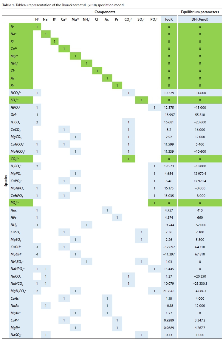
To discover which species could be omitted, a representative composition for an anaerobic digester liquor was set up in PHREEQC, and run for three pH values covering the range that the anaerobic digestion model might be expected to encounter (5, 7 and 9). Species were selected that contributed at least 2% to the inventory of any component in at least one of the model runs. So, for example, the species NaHCO₃had to amount to at least 2% of the total Na⁺, H⁺ or CO₃^2- in at least one of the simulated solutions. The 42 ionic species that were selected in this way were: H+, Na+, K+, Ca++, Mg++, NH₄+, Cl^-, Ac, Pr^-, HAc, HPr, NH₃, HCOf, SO₄²-, HPO₄²-, OH', H₂CO₃, CO₃²-, CaCO₃, MgCO₃, CaHCO₃+, MgHCO₃+, H₂PO₄-, MgPO₄, CaPO^--, MgHPO₄, CaHPO₄, CaSO₄, MgSO₄, CaOH+, MgOH+, NH₄SO₄^- NaHPO₄, NaCOf, NaHCO₃, MgH₂PO₄+, CaAc+, NaAc, MgAc+, CaPr+, MgPr+ and NaSO₄~, where the last 24 in the list are often referred to as ion pairs. Note that, as in the previous papers in this series, species are italicized to distinguish them from components.

Table 1 presents the reaction scheme in a form known as a tableau, which is similar to the Gujer matrix for biological reactions. The matrix contains the stoichiometric coefficients for the formation reaction of each species from its components, and the two rightmost columns hold the thermodynamic constants for each species at 25°C or 298.15°K (obtained from the minteq.v4.dat database).

This selection of components and species still leads to quite a complex model, requiring the simultaneous solution of 42 nonlinear equations. Whether this level of complexity is really required for the anaerobic digestion model is a question that would require a great deal of investigation to answer fully. If alkalinity and pH predictions were the only issues, one could dispense with most of the ion pair species without serious consequences. However, the prediction of whether a precipitate will form or not is quite sensitive to the ion pairs (Solon et al., 2015). As will be discussed in the next section, the extra computational burden of adding species is not great, so we have preferred to err on the side of greater complexity.

It should be mentioned that some authors (e.g. Flores-Alsina et al., 2015) prefer a different formulation of the set of speciation equations, in which H⁺ in the tableau is replaced by the charge balance over the remaining set of components. This is simply a linear transformation of the set of variables, and is entirely equivalent. The motivation for using it seems to be that [H+] is not measurable, whereas the charge balance is a linear combination of measurable quantities. However, this apparent advantage is only fully realised when dealing with synthetic solutions made up from pure chemicals. Measurements on wastewater samples very seldom cover all the ions present, and, even when they do, measurement errors upset the charge balance. The solution state is very sensitive to the H⁺ concentration, so the measured charge balance cannot be used to infer it reliably; consequently, further considerations have to be used to establish an appropriate charge balance, exactly parallel to those discussed in relation to [H⁺], in the later section of this paper, on using speciation with composition measurements.

The speciation algorithm

As mentioned previously, the principles of ionic speciation are well established: they are set out in Stumm and Morgan (1996). The concentrations of the 42 ionic species are related to the concentrations of the 12 components by a set of 12 stoichiometric balances, together with a set of 30 equilibrium relationships which form a set of simultaneous algebraic equations. The equilibrium relationships are formulated in terms of species activities, which are related to their concentrations by activity coefficients.

In the set of equations that constitute the model, the balance equations are linear, but the equilibrium relationships are nonlinear. For example, consider the equations for propionate Pr^-(a conveniently simple example, since the model has only four species containing Pr^-). The balance equation is:

In Eq. 1 the square brackets indicate molal concentrations, italics indicate species, and Roman typeface indicates a component. [Pr^-] is also referred to as a total concentration, as it is the sum of the concentrations of all species present that include Pr^-.

There is one equilibrium relationship for each of the species formed from more than one component (e.g. HPr, CaPr+). Take HPr, for example. Its entry in Table 1 corresponds to the formation reaction H+ + Pr^- HPr, with the corresponding equilibrium relationship:

In Eq. 2, {...} indicates the activity of the species, and K_HPr is an equilibrium constant, which is a function of temperature only, and can be calculated from the thermodynamic parameters in Table 1.

The activities are related to molal concentrations by activity coefficients, e.g.

Equation 4 can be dimensionally confusing, since {Pr^-} and y_Pr are dimensionless, whereas [Pr^-] has dimensions of mol/kg. This is because there is a hidden term - the complete form is:

where the subscript O indicates the species in a standard state which is defined so that [i_O] = 1 mol/kg for all species i. This definition effectively sets the value of the equilibrium constant (e.g. K_HPr in Eq. 2). By convention [i_O] = 1, whatever concentration units are used, so the form of Eq. 4 remains the same if the units are changed; however, the equilibrium constant value changes. So it is critical to use K values that correspond to the concentration units of the model.

Activity coefficients of each species were modelled using the Davies equation (Stumm and Morgan, 1996).

In Eq. 5, I is the ionic strength of the solution I = Σ,[i]z,_i² and z, is the ionic charge on species i. A is the Debye-Hückel constant, which is, in fact, not strictly constant, but a function of temperature.

e is the dielectric constant of water, 78.49 at 25°C, T is the absolute temperature.

The Davies equation is considered to be valid for I < 0.5 mol/kg (Solon et al., 2015)

The equations similar to Eqs 2 and 4 are substituted into Eq. 1 to eliminate all but one of the species containing Pr^-, for example:

The effect of applying this transformation to all the component balances is to reduce the number of simultaneous equations to be solved numerically from 42 to 12. The set of species concentrations remaining after the reduction ([Pr], [H+], [Ca²+], [Mg²+] etc.) is termed the primary search variables or master species for the numerical solution of the equations. Once these core equations have been solved for the master species concentrations, all the remaining species concentrations can be calculated explicitly from the equilibrium equations similar to Eq. 2. It is always possible to do this reduction of variables, so that the number of equations needing simultaneous solution is the number of components in the model. This means that the computational burden of extra species for a given set of components is relatively small.

Computational considerations

Minimising the computational burden is important, since the speciation calculation is performed at each integration step during the numerical solution of the model balance equations. In fact, when using an integration algorithm with variable time-step control, there are additional trial evaluations within an integration step. There are three particularities of the speciation calculation that can be exploited.

Firstly, because the solution composition evolves with time, the solution obtained at the previous time step provides an excellent initial guess for the following time step. When designing a numerical algorithm, there is generally a trade-off between the number of iterations required for convergence, and the complexity of the calculations within an iteration. So, we kept the solution variables in memory between integration steps as estimates for the next step, and used a relatively unsophisticated solution algorithm, i.e., a secant search for [H+], and successive substitution for the other 11 search variables. Flores-Alsina et al. (2015) used an alternative algorithm, which we have also implemented in a later version of our speciation routine: a classic multivariate Newton-Raphson (Press et al., 2007) with analytic evaluation of the Jacobian matrix (see Appendix B for details).

There is obviously a problem at the first integration step, since there is no previous solution to use as an initial estimate. The second useful characteristic is that the 12 primary search variables (master species concentrations) must have values between zero and the corresponding component concentration. This makes it relatively easy to generate an adequate starting guess for the variables. Since this happens only once at the beginning of a simulation, it does not matter much that a larger number of iterations is required for convergence during this initial step. Typically the solution converges in 10 to 30 iterations for the first step, but 3 to 5 iterations during subsequent steps of a simulation.

This leads to the last particularity, the choice of the species concentrations that constitute the primary search variables. The speciation works best, both in terms of the rate of convergence and the accuracy of the solution, if the master species concentrations that the algorithm solves for are the dominant ones for their components. For example, under most circumstances carbonate in an anaerobic digester liquor is predominantly in the HCO₃^-form. Similarly, HPO₄^2-is usually the dominant species for the phosphate system. Thus, we exploit the fact that the range of conditions under which an anaerobic digester operates is relatively limited, and choose search variables accordingly.

The one component that cannot be handled in this way is H+. Although most H+ is usually complexed with weak acid anions (in most wastewaters it is predominantly present as HCOf) an algorithm that chose HCO₃^-as a master species would be unable to deal with a solution that has no carbonate present. Since it comes from the solvent water, H+ is always present, although its concentration may be very low. The problem of very low concentrations can be circumvented by a logarithmic transformation; however there would be an undesirable computational penalty in evaluating logarithms and exponentials. Fortunately, the extra computation can be minimised. Evaluating a term in the transformed Jacobian = ^x^ adds only a single multiplication per term, and when one has to apply the exponential correction, one can use the first-order series approximation exp (Sx) ~ 1+ Sx, which becomes increasingly accurate as the solution converges, i.e. Sx - 0.

Thus, the set of master species adopted was H+, Na+, K+, Ca++, Mg++, NH+, CI^-, Ac^-, Pr^-, HCO₃, SO/- and HPO^2-.

Using speciation with composition measurements

Up to this point, the discussion has focused on speciation calculations during a simulation, where component concentrations are established by material-balance calculations. It is also necessary to use speciation calculations to transform measured compositional data into compositions in terms of model components, that can be used as input to the material balances, or to compare with model outputs. Measurement aspects are discussed in Part 4 (Ekama et al., 2022); here we briefly outline the use of the speciation routine to implement the calculations.

A typical set of measurements on a wastewater sample will not provide a complete description of its composition. Leaving aside the complex dissolved and particulate organic content, the inorganic ionic composition will be represented by some measured component concentrations (e.g. phosphate, sulphate, chloride, sodium, calcium), together with pH and alkalinity, which are summary indicators that reflect the presence of a complex of components. Of the components that strongly affect pH and alkalinity, H+ cannot be measured directly, and CO₃^2- is not commonly measured directly.

The problem that pH measurements pose for modellers is that pH is not a conserved quantity, and so cannot be used directly in material balance calculations. The component H+ is conserved, but cannot be measured directly. Thus it is necessary to use a speciation model to convert pH and alkalinity measurements to equivalent H+ and CO₃^2- concentrations, which can then be used in mass balance calculations. This essentially involves a trial-and-error search for the H+ and CO₃^2- component concentrations that match the measured pH and alkalinity. This approach is used by MINTEQA2 (Allison et al., 2009) and PHREEQC (Parkhurst and Appelo, 2013) and was adopted in the PWM_SA model by Ikumi et al. (2015), of which PWM_SA_AD is a sub-model and uses the same ionic speciation routine (Brouckaert et al., 2010).

However, pH and alkalinity are not functions of just [H+] and [CO₃^2-]. They depend on the whole composition of the solution, which theoretically requires the measurement of all solute concentrations. This is very seldom feasible. However, the effects of other dissolved ions on pH and alkalinity vary greatly, so some are more important to get right than others. The anions of weak acids such as phosphate, sulphide and acetate, and the cations of weak bases such as ammonia, are critical, because they associate with H⁺ and contribute to the measured alkalinity. Anions of strong acids (e.g. chloride and sulphate) and cations of strong bases (e.g. sodium, potassium, calcium and magnesium) have a minor influence on the H+ activity coefficient via their contributions to the ionic strength of the solution, and are much less critical. Thus, while it is important to have the correct concentrations for the weak acid and base components, it may be adequate for modelling purposes to use the ionic strength to summarise the effect of the rest of the inorganic ions. There are empirical correlations to estimate ionic strength from measured electrical conductivity (e.g. Bhuiyan et al., 2009). This kind of approximation is obviously not appropriate when modelling precipitation that involves one or more of the strong acid or base ions, for example Ca²⁺, in which case it is important to have the speciation of Ca²+ right, including ion pairs, such as CaSO₄and CaPO, that reduce the free calcium ion concentration [Ca²⁺].

Alkalinity

Alkalinity was introduced in Part 1 (Brouckaert et al., 2021a) and further discussed in Parts 2 (Brouckaert et al., 2021b) and 4 (Ekama et al., 2022); however, a definition of alkalinity for modelling purposes needs to be chosen. The options are:

(a) From a laboratory measurement point of view, alkalinity is the result of a titration with HCl to an endpoint somewhere between pH 3.5 and 4.5 (the operational definition, according to Snoeyink and Jenkins, 1980). For modelling purposes, to use this directly as the definition is very awkward, as it effectively involves simulating the titration, i.e., solving for the amount of H⁺ and Cl^- to be added to achieve the required pH.

(b) Alkalinity could be defined in terms of species present in the solution in question, by considering all the species that would be protonated at pH 3.5 and calculating the difference between their proton content in the solution and in their fully protonated form.

(c) It could also be calculated from the component concentrations, by subtracting the total H⁺ concentration from the weighted sum of total anion component concentrations which represents the H⁺ that they would contain when fully protonated.

Snoeyink and Jenkins (1980) call (b) and (c) analytical definitions of alkalinity. In the context of a mass-balance model, that works in terms of component concentrations, calculating the alkalinity from the operational definition given in (a) would require one to do speciation calculations for the solution at both its original composition and at the titration endpoint composition (and at a number of other compositions during the search for the endpoint); Definition (b) would require speciation of the original composition only; while Definition (c) requires no speciation calculation at all.

A simulation of the titration of a solution with composition as shown in Table 2 was used to compare the values of alkalinity calculated according to the three different definitions. Note that the composition is specified in terms of component concentrations, not species concentrations. The water content of the solution is implicit in the mol/kg units.

 

 

The resulting total alkalinity (Alk) values are:

Definition (a): 0.016853 M or 843 mg/L as CaCO₃

Definition (b): 0.016874 M or 844 mg/L

Definition (c): 0.016877 M or 844 mg/L

The differences between these values are negligible compared to uncertainties in experimental determinations. Thus Definition (c), based purely on component concentrations, is the obvious one to choose for a computational model.

For the solution of Table 2, the expression for the alkalinity according to Definition (c) in terms of component concentrations is:

where the Alk uses the alkalinity of the orthophosphate system expressed with respect to the HpO₄species. The total alkalinity, according to Definition (c), is simply a linear combination of component concentrations, which shows that it is a purely stoichiometric quantity expressed with respect to a selected set of reference species. Indeed, The IWA ASM series of models (Henze et al., 2000) considers total alkalinity as a component in itself.

The expression for alkalinity of the example solution according to Definition (b), in terms of species concentrations, is:

In Eq. 9 [H+], for instance, represents the concentration of free hydrogen ion (species concentration: 4.899 x 10^-8 M for this example, corresponding to pH 7.4) rather than [H+], the total hydrogen ion concentration (component concentration: 0.020578 M) as in Eq. 8.

Equation 9 can be simplified by including only the main contributing species, i.e., omitting the ion pairs,

Under the range of conditions encountered in anaerobic digesters, the difference between Eqs 9 and 10 will be less than 1%.

Note that terms involving [Pr^-] and [HS^-] have been included in Eqs 8 to 10 for completeness - they are all zero for the example solution of Table 2. [HS^-] is also always zero for the speciation model of Table 1, as it does not include HS^- as a component.

 

CONCLUSIONS

Models of biological processes often need to include interactions with inorganic ionic species, in order to represent phenomena such as acid/base reactions, gas transfer and precipitation. Particularly for the acid/base reactions, an equilibrium sub-model is appropriate, because they have time scales that are orders of magnitude shorter than the biological reactions. The situation is not as clear-cut for redox and phase-transfer reactions which may depart significantly from equilibrium, and so may be more appropriately included in the kinetically limited sub-model. In setting up an equilibrium speciation sub-model, modellers can take advantage of the knowledge and experience contained in freely available modelling software such as MINTEQA2 and PHREEQC. It is possible to couple such software directly to a model: for example, PHREEQC provides a programming interface to access its functions. However, there are computational advantages to customising the speciation algorithm for the range of conditions expected for a given biological system.

The aquatic species and components included in the model must be chosen carefully according to what phenomena the model is required to represent. The established aquatic chemistry models provide useful guides; however, because they are designed to be used in a very wide range of contexts, they tend to suggest model structures that are more complex than necessary for a given process model, but have the advantage of reliability. However, one can reduce the complexity of the model, while using PHREEQC or MINTEQA2 as a reference to check the accuracy of key outputs.

 

ABBREVIATIONS

ASM activated sludge models

IWA International Water Association

PWM_SA_AD University of Cape Town/University of KwaZulu-Natal Anaerobic Digestion Model which is a subset of the plant wide PWM_SA model

 

SYMBOLS

A Debye-Hückel constant

Alk_t total alkalinity in solution relative to H₂CO₃/H₂PO₄^-/ NH₄+/H₂S/HAc

K¡ equilibrium constant for the formation reaction for species i

I ionic strength, mol/kg

z_i ionic charge on species i

[i] molal concentration of component i, mol/kg

[i] molal concentration of species i, mol/kg

{i} activity of species i, dimensionless

AH enthalpy change of reaction, J/mol

y_i activity coefficient of species i

 

REFERENCES

ALLISON JD, BROWN DS and NOVO - GRADAC KJ (2009) MINTEQA2. https://www.epa.gov/eam/minteqa2-equilibrium-speciation-model (Accessed 5 June 2019).         [ Links ]

BHUIYAN IH, MAVINIC DS and BECKIE RD (2009) Determination of temperature dependence of electrical conductivity and its relationship with ionic strength of anaerobic digester supernatant, for struvite precipitation. J. Environ. Eng. 135 1221-1226. https://doi.org/10.1061/(ASCE)0733-9372(2009)135:11(1221)        [ Links ]

BROUCKAERT CJ, IKUMI DS and EKAMA GA (2010) A 3 phase anaerobic digestion model. Proceedings 12^th IWA Anaerobic Digestion Conference (AD12), Guadalajara, Mexico, 1-4 Nov 2010.         [ Links ]

BROUCKAERT CJ, BROUCKAERT BM and EKAMA GA (2021a) Integration of complete elemental mass-balanced stoichiometry and aqueous-phase chemistry for bioprocess modelling of liquid and solid waste treatment systems - Part 1: The physico-chemical framework. Water SA. 47 (3) 276-288. https://doi.org/10.17159/wsa/2021.v47.i3.11857        [ Links ]

BROUCKAERT CJ, EKAMA GA and BROUCKAERT BM (2021b) Integration of complete elemental mass-balanced stoichiometry and aqueous-phase chemistry for bioprocess modelling of liquid and solid waste treatment systems - Part 2: Bioprocess stoichiometry. Water SA. 47 (3) 289-308. https://doi.org/10.17159/wsa/2021.v47.i3.11858        [ Links ]

EKAMA GA, BROUCKAERT CJ and BROUCKAERT BM (2022) Integration of complete elemental mass-balanced stoichiometry and aqueous-phase chemistry for bioprocess modelling of liquid and solid waste treatment systems - Part 4: Aligning the modelled and measured aqueous phases. Water SA 48 (1) 21-31. https://doi.org/10.17159/wsa/2022.v48.i1.3322        [ Links ]

FLORES-ALSINA X, KAZADI MBAMBA C, SOLON K, VRECKO D, TAIT S, BATSTONE DJ, JEPPSSON U and GERNAEY KV (2015) A plant-wide aqueous phase chemistry module describing pH variations and ion speciation/pairing in wastewater treatment process models. Water Res. 85 255-265. https://doi.org/10.1016/j.watres.2015.07.014        [ Links ]

HENZE M, GUJER W, MINO T and VAN LOOSDRECHT M (2000) Activated sludge models ASM1, ASM2, ASM2d, and ASM3. IWA Scientific and Technical Report. IWA, London. https://doi.org/10.2166/wst.1999.0036        [ Links ]

LOEWENTHAL RE, KORNMULLER URC and VAN HEERDEN EP (1994) Modelling struvite precipitation in anaerobic treatment systems. Water Sci. Technol. 30 (12) 107-116. https://doi.org/10.2166/wst.1994.0592        [ Links ]

LIZZERALDE I, BROUCKAERT CJ, VANROLLEGHEM PA, IKUMI DS, EKAMA GA, AYESA E and GRAU P (2014) Incorporating aquatic chemistry into wastewater treatment process models: a critical review of different approaches. In: Proceedings 4th IWA/ WEF Wastewater Treatment Modelling Seminar. WWTmod2014, Spa, Belgium, 30 March - 2 April 2014. 227-232.         [ Links ]

PARKHURST DL and APPELO CAJ (2013) PHREEQC (Version 3)-- A computer program for speciation, batch-reaction, one-dimensional transport, and inverse geochemical calculations. URL: https://www.usgs.gov/software/phreeqc-version-3 (Accessed 5 June 2019).         [ Links ]

PRESS WH, TEUKOLSKY SA, VETTERLING WT and FLANNERY BP (2007) Numerical Recipes (3^rd edn). Cambridge University Press, Cambridge.         [ Links ]

SNOEYINK VL and JENKINS D (1980) Water Chemistry. John Wiley and Sons, New York.         [ Links ]

SOLON K, FLORES-ALSINA X, KAZADI MBAMBA C, VOLKE EIP, TAIT S, BATSTONE D, GERNAEY KV and JEPPESON U (2015) Effects of ionic strength and ion pairing on (plant wide) modelling of anaerobic digestion. Water Res. 70 235-245. https://doi.org/10.1016/j.watres.2014.11.035        [ Links ]

STUMM W and MORGAN JJ (1996) Aquatic Chemistry: Chemical Equilibria and Rates in Natural Waters. John Wiley and Sons, New York.         [ Links ]

 

 

Correspondence:
CJ Brouckaert
Email: brouckae@ukzn.ac.za

Received: 3 July 2019
Accepted: 29 December 2021

 

 

APPENDIX A

Phase transfer reactions

The anaerobic digestion model of Brouckaert et al. (2010) considered three phases, gas liquid and solid, with phase-transfer reactions distributing material between them. These phase-transfer reactions were represented as kinetically controlled, and so not handled by the equilibrium speciation sub-model, which dealt with the liquid phase only. However, the rate expressions for the phase-transfer reactions involved liquid species concentrations that required the equilibrium speciation sub-model for their evaluation.

Gas transfer

The evolution of CO₂ is used as the example. The transfer reaction is:

Dissolved carbonate exerts an equilibrium partial pressure P_CO2eq which can be represented as

K_H is the Henry's Law Constant, and can be calculated from thermodynamic data as a function of temperature. The rate of Reaction A1 is then modelled as:

P_CO2eqis calculated from the liquid equilibrium speciation, whereas P_CO2 is calculated from the gas phase mass balance. The rate constant k_CO2 is a model parameter.

Precipitation/dissolution

This follows a similar treatment. Consider the precipitation of CaCO₃ as the example.

The precipitation/dissolution reaction is:

The solution is saturated with respect to CaCO_3W when

K_{CaCO3_sat} is a saturation coefficient and can be calculated from thermodynamic data as a function oftemperature. {Ca²+} • {CO₃^2-} is termed an ion product IP_caco3, and is calculated from outputs of the equilibrium speciation sub-model.

When (IP_caco3> K_{caco3_sat}), CaCO_3(s) will precipitate, and when (IP_caco3< K_{caco3_sat}) any CaCO_3(s)that is present in the reactor will dissolve. So the rate of Reaction A4 is modelled as proportional to (IP_caco3^-K_{caco3_sat})^.

 

APPENDIX B

Implemention of the Newton-Raphson algorithm for ionic speciation

The Newton-Raphson algorithm solves a set of non-linear equations f(x) = 0 iteratively by linearising the equations at successive trial points. Here f, x, and 0 are vectors - i.e.

The superscript T indicates that the vectors are transposed - i.e. they are column vectors.

Linearisation at any trial point x is achieved by evaluating the Jacobian matrix

For the present problem, x is the vector of 12 master species concentrations, and f is the vector of errors in the 12 component balances. The vector of corrections to x is given by the solution to the set of linear equations (B3), which can be solved numerically using a standard algorithm.

The formulation of the Newton-Raphson scheme for the speciation problem can be illustrated with reference to Eq. 7, which is one of the 12 equations to be solved. We rearrange it as:

Here f_Pris the error in the propionate balance, which, together with the 11 other component balance errors, should be driven to zero by a proper choice of values of [Pr^-], [H+], [Ca²+] and [Mg²+] (and eight other concentrations which appear in the other balance equations). [Pr^-] is a constant, and the K values, although not strictly constant, can be considered approximately constant during a single iteration.

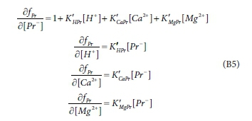
The terms in the Jacobian matrix are the derivatives of the error equations with respect to the variables. From Eq. B4:

If one chooses to use the logarithmic transformation, Eq. B3 becomes:

where Eq. B5 becomes

In this case, once the vector of values for 8 ln x has been obtained from the solution of B6, the correction to the i^thvariable during the j^th iteration is applied as:

which is equivalent to:

This completely avoids evaluation of the ln and exp functions.