RESEARCH PAPER

 

Integration of complete elemental mass-balanced stoichiometry and aqueous-phase chemistry for bioprocess modelling of liquid and solid waste treatment systems - Part 1: The physico-chemical framework

 

 

CJ Brouckaert^I; BM Brouckaert^I; GA Ekama^II

^IWater, Sanitation and Health Research and Development Centre, School of Engineering, University of KwaZulu-Natal, Durban, 4041, South Africa
^IIWater Research Group, Department of Civil Engineering, University of Cape Town, Rondebosch, 7700, South Africa

Correspondence

 

 

---

ABSTRACT

Bioprocesses interact with the aqueous environment in which they take place. Currently integrated bioprocess and three-phase (aqueous-gas-solid) multiple strong and weak acid/base system models are being developed for a range of wastewater treatment applications, including anaerobic digestion, biological sulphate reduction, autotrophic denitrification, biological desulphurization and plant-wide wastewater treatment systems. In order to model, measure and control such integrated systems, a thorough understanding of the interaction between the bioprocesses and aqueous-phase multiple strong and weak acid/bases is required. This first in a series of five papers sets out a conceptual framework and methodology for deriving bioprocess stoichiometric equations. It also introduces the relationship between alkalinity changes in bioprocesses and the underlying reaction stoichiometry, which is a key theme of the series. The second paper develops the stoichiometric equations for the main biological transformations that are important in wastewater treatment. The link between the modelling and measurement frameworks, which uses summary measures such as chemical oxygen demand (COD) and alkalinity, is described in the third and fourth papers. The fifth paper describes an equilibrium aquatic speciation algorithm which can be combined with bioprocess stoichiometry to provide integrated models of wastewater treatment processes.

Keywords: Modelling framework; stoichiometry; bioprocesses; aquatic chemistry; alkalinity

---

 

 

INTRODUCTION

This is the first in a series of five papers that aim to set out a consistent approach to modelling biological processes involved in wastewater treatment. Part 2 appears alongside Part 1 in this issue, and Parts 3, 4 and 5 will be published in later issues of Water SA.

The governing relationships of steady state and dynamic kinetic models of aerobic or anaerobic biological treatment systems fall into three major categories, viz.

• Continuity (mass, energy and momentum balances)

• Equilibria

• Kinetics

Although every reaction process is governed by all these relationships, models often do not explicitly take non-limiting factors into account. Thus, mass balances must always be included, but momentum and energy balances can often be left out (as in this series of papers). The situation with respect to kinetic and equilibrium relationships is more complex, because biochemical models usually represent a network of transformation processes, some of which may be kinetically limited, others equilibrium limited, and others mass-balance limited. Representing a biochemical reaction always involves a stoichiometric equation (mass balance) which may need to be coupled with a kinetic equation and/or equilibrium relationships. A number of models in the literature reflect a clear divide between kinetically controlled biological reactions (e.g. methanogenesis) that are far from equilibrium, and very fast acid/base reactions that are assumed to be at equilibrium (e.g. the dissociation of carbonic acid).

Early dynamic and steady-state models for the activated sludge (AS) system (Dold et al., 1980; WRC, 1984) considered only the bioprocesses and comprised only the COD mass-balanced kinetically controlled transformations, as well as N (and P) mass balances, but omitted the C, H and O mass balances. The C balance was not included because most of the CO₂ produced is stripped out by the aeration system and it is assumed that its effect on the reactor pH can be neglected. Consequently, this model did not include speciation or pH prediction. Instead, the variable Alk tracked changes in alkalinity due to the removal and production of strong acids by the bioprocesses, like nitrification and denitrification. A large decrease in Alk to below 50 mg/L as CaCO₃ was a flag that pH problems could arise in the reactor (WRC, 1984; Henze et al., 2008).

The importance of including weak acid/base chemistry in biological process models was discussed by Batstone et al. (2012). In anaerobic digestion (AD) models, the C-balanced stoichiometry and weak acid/base chemistry parts of models need to be included because the AD methanogens are very sensitive to pH, and the CO₂ and CH₄ gas produced establish a CO₂ partial pressure (p_CO2) in the AD head space that, together with the aqueous phase alkalinity, establishes the AD pH (McCarty, 1975; Andrews and Graef, 1971; Speece, 2008; Sötemann et al., 2005a, b, c). Recently these developments in AD modelling have also been applied to activated sludge system models to enable the creation of plant-wide wastewater treatment models with complete CHONPS, charge and COD mass-balanced stoichiometry and three-phase (aqueous-gas-solid) mixed weak (and strong) acid/base chemistry to predict reactor (AD and AS) pH and mineral precipitation (Sötemann et al., 2005c; Takacs and Vanrolleghem, 2006; Grau et al., 2007; Brouckaert et al., 2010; Ikumi et al., 2011, 2014, 2015). How this integration is achieved in different steady-state and dynamic bioprocess aqueous phase models is the subject of this series of papers.

Ekama and co-workers (e.g. Sötemann et al., 2005b; Ekama, 2009; Poinapen and Ekama, 2010a; Lu et al., 2012) have developed a set of steady-state anaerobic digestion models in which the aquatic chemistry aspects are integrated into the model by expressing the stoichiometric biological half-reactions in terms of the dominant weak acid and base species expected to be present under particular conditions. The formulation of these half-reactions is based on the approach of McCarty (1975), and uses prior knowledge of the weak acid/base chemistry of the various biological treatment processes under typical operating conditions to determine which species to include. This results in a much simpler model that can be solved explicitly. Part 2 of this 5-part series develops this approach in detail (Brouckaert et al., 2021).

The disadvantage of this approach to predicting speciation is that it makes assumptions about the distribution of weak acid/base species that are only valid for a fairly narrow range of conditions (e.g. near-neutral pH). It is therefore not appropriate for dynamic scenarios and deviations from normal operating conditions, e.g., anaerobic digester failure. This is particularly an issue for anaerobic digestion, the performance of which is sensitive to pH fluctuations. Nevertheless, the steady-state models developed using this approach have important practical applications in design and capacity estimation, and understanding the chemistry on which they are based is critical in understanding the role of alkalinity in the design and control of biological processes. Therefore, it is important to understand both how these models work and their limitations.

These limitations have been addressed by various researchers in two different ways:

1.Musvoto et al. (2000a,b; Sötemann et al., 2005a,c; Poinapen and Ekama, 2010b) included dynamic equilibrium speciation equations (very fast forward and reverse reactions) as part of the kinetic structure of their anaerobic digestion model.

2.More recent models have tended to use algebraic algorithms to solve the weak acid/base chemistry and calculate the pH external to the kinetic model (IWA ADM1, Batstone et al., 2002; Serralta et al., 2004; Barat et al., 2011; Lizzaralde et al., 2015; Solon et al., 2015).

 

DEVELOPING A GENERALIZED APPROACH TO MODEL INTEGRATION

Batstone et al. (2012) argued that an incremental approach to incorporating aquatic chemistry into biochemical process models is inefficient. Modelling the interactions of inorganic aqueous components is a well-established discipline, with a comprehensive conceptual framework. They concluded that a similar framework should be developed for bioprocess modelling that encompasses both the biochemical and inorganic aspects. However, the existing biological and inorganic modelling frameworks have different characters, which are shaped by their respective subject matter. An integrated framework obviously needs to reflect both.

Broadly speaking, inorganic aquatic chemistry models (e.g. MINTEQA2, PHREEQC, etc.) tend to be based on precise stoichiometry and thermodynamic data, whereas current biochemical models (e.g. ASM series models, Henze et al., 2000) tend to be based on summary chemical characteristics (such as chemical oxygen demand: COD), and kinetic formulations. This reflects the fact that biochemistry is concerned with enormously complex organic molecules, that are maintained in states very far from chemical equilibrium by kinetic factors. Conversely, most aquatic chemistry models provide comprehensive support for reaction equilibria, but no special support for kinetically limited processes. Thus, for example, redox reactions are frequently not at equilibrium in aquatic systems, and the kinetic factors governing them have to be established experimentally on a case-by-case basis, just as with biochemical processes. Indeed, some are even catalysed by biochemical processes, such as sulphate to sulphide reduction or ammonia to nitrate oxidation.

These considerations suggest that it would be impractical for an integrated modelling framework to have a uniform approach to all transformation processes and their components, at least for the foreseeable future. A hybrid approach is needed, for which the main new consideration is establishing the links between biological and inorganic processes. There are two major issues to be addressed:

• Precise stoichiometry for biological processes to match that for inorganic processes.

• The simultaneous representation of kinetically limited processes and equilibrium limited processes.

These papers are chiefly about the stoichiometry, which needs to take account of the requirements of equilibrium and kinetic formulations. Part 2 deals with the development of precise stoichiometry in detail (Brouckaert et al., 2021). Part 1 makes two further contributions:

• Expressing the stoichiometric balances in terms of components used by the equilibrium speciation model in order to facilitate the integration of the two models.

• Using a convenient matrix method to solve the stoichiometric balances.

The general methodology adopted here can be summarised as follows (section headings are shown in parentheses):

• Determine which processes will be represented by which type of model (Kinetic and equilibrium models).

• Select a set of model components which are used to describe the material content of the system which are the inputs to the speciation model (Components and species in aquatic process models).

• Express the biological reaction stoichiometry in terms of the speciation model components (Stoichiometry of biological components and reactions); this section also presents a compact matrix method for solving for the stoichiometric reaction coefficients.

The algorithm used to calculate the equilibrium speciation is presented in Part 5 of the series. A more detailed discussion and practical demonstration of the principles and tools presented in this paper can also be found in a set of open access course materials on the integration of aquatic chemistry with bioprocess models developed under South African Water Research Commission Project K5/2125. The entire course is available at https://washcentre.ukzn.ac.za/bio-process-models/. Practical implementations of models using these principles are presented by Ikumi et al. (2015).

A simulation model must capture detailed physical knowledge about a system. This paper, Part 1, presents a framework for organising such knowledge about a biochemical system rather than any specific model. The specific information required to build an integrated biochemical model includes which sub-processes are limiting, which transformations need to be explicitly represented in the model, and what reactants and products are involved. The tools presented in this section are applicable to any biochemical system. However, because of the importance of pH in maintaining stable digester operation, many of the examples presented relate to anaerobic digestion.

It is a characteristic of a conceptual framework that there are forward and backward linkages between its parts, and that it needs to be understood in its entirety to be fully useful. A written account is necessarily sequential, and cannot convey this integrated understanding directly - it has to be synthesized by the reader. This means that the relevance of some aspects may not immediately evident when they are first introduced, and earlier sections may need to be revisited to fully grasp their connections with later sections.

 

CLASSIFICATION OF MODELS

The simulation of chemical and biochemical processes involves two basic kinds of calculations: determining what material will be present at a particular location and time (mass balancing), and determining the physical state that it will take on at that point (speciation).

Stumm and Morgan (1996) classify aquatic models into two basic kinds:

•Continuous open systems, which exchange material with their surroundings, and consequently vary their composition through both flows and reactions.

• Closed systems, with fixed material content, so that composition can only vary with reactions and internal processes.

Chemical and biochemical process simulators almost always employ continuous open system models. A typical model configuration has a set of unit modules which represent control volumes linked by flows. A unit module balances inflows, outflows and internal reactions to determine the composition and characteristics of the material in its control volume, either as a function of time or at steady state.

 

KINETIC AND EQUILIBRIUM MODELS

Particularly for biochemical models, the internal processes are most often represented as rate-limited reactions, requiring kinetic information for their simulation. However, where process kinetics are not limiting, it is appropriate to use an equilibrium model. This occurs as an asymptotic approximation, when the time scale of the internal transformations becomes very short compared to the time scale of the external flow. In this asymptotic limit, the model becomes one of a closed system. When the rates of aquatic reactions making up the model vary enormously, it becomes appropriate to model some processes using a kinetic formulation, and others using an equilibrium formulation in the same unit module. This means that the same control volume will be treated simultaneously as an open system for some processes, and a closed system for others. For the equilibrium sub-system, the material content is 'frozen in time' in order to calculate its state. The practical consequence is that the equilibrium speciation only takes account of the instantaneous material content of the system, ignoring time derivatives and material flows across its boundaries.

To illustrate the concepts of kinetic and equilibrium limited processes, consider the hydrolysis of urea:

The overall reaction could be considered as kinetically limited or mass-balance limited, depending on the time scale of interest. Urea hydrolysis is typically kinetically limited by bio catalysis, but, given sufficient time, proceeds to completion. Therefore, depending on the time scale of the model, the concentrations of reactants/products over relatively short time scales may be described by reaction kinetics, and over relatively long time scales by mass balance.

However, the products of the hydrolysis reaction (NH₄⁺ and CO₃⁼) are also involved in a parallel set of aqueous phase ionic reactions, of which the following are a sample:

The ionic reactions in Reaction 2 are very rapid compared to urea hydrolysis, and reach equilibrium almost instantaneously. Furthermore, at equilibrium these reactions can have significant reagent concentrations remaining, which are determined by a set of equilibrium relationships. The equilibrium speciation represented by Reaction 2 establishes the pH which affects the kinetics of urea hydrolysis (Fidaleo and Lavecchia, 2003). Therefore, if the hydrolysis process is kinetically limited, an iterative procedure is required to establish both the solution pH and extent of the hydrolysis reaction. Finally, it is important to note that considering a reaction as either equilibrium limited or kinetically limited is a modelling approximation which depends on the model context.

 

COMPONENTS AND SPECIES IN AQUATIC PROCESS MODELS

A number of different conventions are used to represent aqueous composition in the various models that are currently in use. This section aims to provide a general perspective on the problem of choosing a set of compositional variables for a model.

The term components will be used to describe those model entities which collectively define the overall material content of a system. This is the same definition of model components which is used in the chemical equilibrium speciation package MINTEQA2 (Allison et al., 2009), and is also equivalent to the meaning of the term components used in biochemical models such as ASM1 (Henze at al., 1987). In the framework presented here, stoichiometric material balances for biochemical transformations are formulated in terms of components (for example, Reaction 1 in the urea hydrolysis example is the stoichiometric balance for the biological transformation part of the model and has been expressed in terms of the model components selected for this system). Species are those molecular entities which are required to describe the actual physical state of the material. The speciated composition of the aqueous phase is used to calculate characteristic solution properties, such as pH and reaction rates, since these generally depend on the actual species present. In the urea hydrolysis example, Eq. 2 describes the formation of the species actually present.

The distinction between components and species as defined here is key to the set-up and solution of the equilibrium speciation models. As discussed earlier, this paper presents a framework for organizing the information required to model a bio-chemical system. Perhaps the most critical part of this knowledge consists of understanding what species and components are relevant for a particular system. Since we focus on the tools for organising the knowledge, we work with an assumption that the biochemical knowledge is already in place. Our theme is that, once we understand the species and components of a system, the framework and its tools will take us a considerable way towards completing the system description.

General note on terminology and notation for components and species

The terms 'component' and 'species' are widely used in the chemistry and modelling literature with meanings that are closely related, but not necessarily identical to the ones used here. For our purposes, they are variables in a computational model, and their characteristics are purely related to the calculations that are performed on them.

Standard chemical notation does not distinguish between components and species; therefore, one has to infer what is meant from the context. For example, if the symbol NH₃ appears in a balanced stoichiometric reaction equation, it usually indicates a component, since the equation represents a mass balance, nothing more. A symbol such as NH_3(aq) or NH_3(g) usually (but not inevitably) refers to a molecular species. There is a move to adopt an unambiguous notation in the specialised modelling literature, but it has not been widely accepted yet. In this series of papers we have elected to follow standard chemical notation, which corresponds to the bulk of the literature. In this Part 1, a chemical formula refers to a component unless explicitly stated otherwise. For clarity, species are in italic font to distinguish them from components.

Components

Most equilibrium speciation algorithms are based on what is referred to as 'Duhem's Theorem' in thermodynamics. In fact, this is not strictly a theorem, as it cannot be proven - rather it is a very abstract and general observation about the behaviour of matter. Smith and Van Ness (2005) state it as follows: 'For any closed system formed initially from given masses of prescribed chemical species, the equilibrium state is completely determined when any two independent variables are fixed.' Note that their use of the word 'species' corresponds to the meaning that has been assigned to 'components' in this series of papers. The 'two independent variables' are commonly taken to refer to temperature and pressure, although any other two independent thermodynamic state variables can be substituted.

Hence, the first task of any equilibrium model is to specify the material content of the system being analysed. Components are the variables used in this specification. There is no necessity for model components to correspond to chemical constituents as they actually exist in the system; they only have to account correctly for the atoms present.

The use of ionic components requires special consideration. Since macroscopic charge imbalances are not possible, ions cannot be independent elements of the system composition. However, electrons within a system re-distribute themselves at the molecular level to form ions. Since ions are persistent features of aqueous solutions, it is convenient to treat them as components. Databases of ionic component properties are readily available which allow modular representations of aquatic systems in terms of these components.

However, because of the overall electro-neutrality requirement, they are not quite independent components. Where a composition is expressed in terms of ionic components, a charge balance has to be imposed as an additional constraint. Since there is only one overall charge balance, it tends to have less and less impact on the model formulation as the number of ionic components in the system increases.

An ionic component is formally a collection of elements with a net charge. Relative to their neutral reference state, each element may have either gained or lost electrons. An element which gains an electron is said to be reduced, and one that loses an electron to be oxidised. The net charge of the ion reflects the net gain or loss of electrons by its elements to other (oppositely charged) ions in the solution. So, the charge can be accounted for by considering electrons as part of the stoichiometric content of the ion. Because the electron content is expressed as relative to the neutral elemental state, it can be either a positive or negative quantity, leading to a negative or positive ionic charge, respectively.

To summarize: components are the variables used to specify the material content of a system. For this purpose they do not need to correspond to molecular species, and so their choice is not unique. Ionic components are constructed by specifying their content in terms of elements plus or minus electrons, with the understanding that a charge balance constraint will be added to complete the system description. The charge balance and the electron balance are identical, apart from reversal of signs, and once the elements and electrons are balanced, oxidation and reduction will also be balanced.

Species

To represent the physical state of the material in the system, it is important to consider the actual molecular configurations of these atoms. Hence model species should correspond to molecular reality as far as possible.

In the equilibrium sub-model, species are related to components by formation reactions as described in Part 5. In some cases, components can correspond to the dominant species present, and this can be used to simplify the model and/or equilibrium speciation calculations. However, in other cases, the component chosen will not correspond to the species expected to be present. For example, total sulphate SO₄^2- and phosphate PO₄^3- present in the system are typical choices for components because they correspond to the quantities measured in a water quality analysis. The sulphate ion SO₄^2- is also the dominant sulphate species present at neutral conditions. However, phosphate occurs predominantly as the species H₂PO₄^- and HPO₄^2- under the same conditions. In general, speciation is the calculation process by which the composition, ultimately reflecting the collection of atoms that make up the system, but usually expressed in terms of component masses, is transformed into one expressed in terms of species masses.

In general, speciation refers to all species, irrespective of whether they take part in equilibrium processes or kinetically limited processes. However, the term is often used as an abbreviation for equilibrium speciation, that is, the distribution of species produced by equilibrium processes.

It important to note that that the distinction between components and species (as defined in this paper) is only useful for equilibrium speciation, since the equilibrium state is determined by the material content of the system only. As discussed above, in an equilibrium system at a given temperature and pressure, Duhem's theorem implies that the state depends only on the material present, therefore the speciated composition at equilibrium does not depend on the choice of model components, provided that the mass of each element and associated electrons present is correctly accounted for. However, Duhem's theorem only applies to the equilibrium sub-system and not to the kinetically controlled part of the model. In the kinetic sub-model, the physical state of the system and how it evolves with time do depend on what molecular species are present. Consequently, the mass balance cannot be decoupled from the speciation for kinetically controlled species. The modelling framework must therefore distinguish between species which are formed by kinetically limited processes, and those that are approximated as formed by equilibrium processes. Examples of the former might be acetate or molecular hydrogen formed as intermediates in anaerobic digestion, while an example of the latter is free hydrogen ion concentration, or equivalently pH.

The presence of kinetically controlled species introduces additional degrees of freedom to the mass balance calculations, which require additional information to specify the composition of the system at any point in time. In the urea hydrolysis example (Eq. 1), the kinetically controlled species urea (CO(NH₂)₂) is treated as a component in mass balance calculations, and as a species in kinetic expressions, and the same model variable can be used to hold its concentration for both purposes. However, it is not directly involved in any equilibrium speciation reactions and therefore does not appear in the equilibrium sub-model at all.

However, some kinetically limited species, in particular organic acid and bases, can be simultaneously involved in both kinetically and equilibrium limited processes. For example, acetic acid is not an equilibrium species under the conditions normally encountered in wastewater treatment. Given sufficient time, it will break down to carbonate, methane and water, as indeed takes place through biological action. However, the dissociation of acetic acid into acetate and hydrogen ion is extremely rapid, and can be modelled as being at equilibrium. As in the urea example, acetate will be treated as a component in the bioprocess stoichiometric balance and as a species in the kinetic sub-model. However, unlike urea, acetate is also included in the equilibrium sub-model. The total acetate present in the system will be a component for input to the equilibrium speciation calculations.

This kind of component requires a modification to the application of Duhem's theorem, in which the kinetically maintained component (e.g. acetate) is treated as though it were a separate element for the purpose of specifying the material content of the equilibrium system. This is because, although acetate consists of C, H and O atoms, which are already present in other system components, we do not include conversion to these components in the equilibrium sub-model, because it does not take place instantaneously. Since most redox reactions are kinetically limited, different redox states of the same element, e.g., sulphate and sulphide, nitrate and nitrite, acetate, propionate, carbonate and methane, are typically represented by separate components.

On the other hand, species such as the free H⁺ ion cannot be independently added or removed from a physical system in practice, so should not be modelled as components, but rather be determined from the components present by a speciation calculation.

It is worth noting that such issues tend to be addressed automatically for aquatic systems by the choice of standard components included in the databases of aquatic chemistry modelling packages such as MINTEQA2 (Allison et al., 2009) and PHREEQC (Parkhurst and Appelo, 2013).

Formulating components for a model

Fundamental considerations place only a few restrictions on how the components should be chosen. Once one has decided what range of compositions should be represented in a model, what strategies could be used to select from the infinite range of possible formulations? The question of alternative choices of components arises primarily for those involved in equilibrium speciation, not for those components governed by kinetics, which have no reason to be different from the species, as in the urea hydrolysis example.

There are two main issues that will influence the choice, and there will usually be some compromise between them:

(a)To make the model as compact and efficient as possible, one would try to reuse as many as possible of the kinetically important species as components. The remaining components required to span the model's compositional space would be chosen purely for their linear independence. (In the H₂O/CO₂ illustrative example above, this corresponds to using CO₂ and H₂O as the components).

(b)The alternative strategy is to use, or select from, sets of components from established models (observing the require-ments for completeness and independence), thereby tapping into the accumulated experience that they represent. This has advantages when it comes to validating the model, in that comparison with previous models is made easier. (In the H₂O/CO₂ illustrative example, this corresponds to using CO₃²⁻, H⁺ and H₂O as the components).

Strategy (a) will tend to produce models that are compact and efficient, but will be more difficult to compare or integrate with each other.

Strategy (b) will tend to produce models that are more widely understood and compatible with each other, at the possible expense of some computational efficiency.

Aquatic chemistry models such as MINTEQA2 and PHREEQC make use of a highly developed system of components and species, supported by extensive thermodynamic databases. These are referred to here as the standard aquatic chemistry components (see Appendix). The component list is carefully designed so that all the components are stoichiometrically independent. This means that any desired system within their scope can be represented simply by including the appropriate set of components. A modeller following strategy (b) need only adopt their system for the inorganic part of the model. This is the approach that is followed in this series of 5 papers. However, examples of the alternative approach will be presented in Part 2 (Brouckaert et al., 2021).

 

STOICHIOMETRY OF BIOLOGICAL COMPONENTS AND REACTIONS

Note that, since stoichiometric biological reaction equations only express element and charge balances, all the chemical symbols in this section (such as CO₂ or CH₃COO^-) represent components, not species.

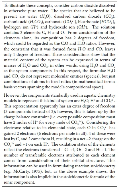
The approach that we propose for setting up the biological reaction stoichiometric balances is based on, and equivalent to, McCarty's (1975) general method for deriving the stoichiometry of biologically mediated reactions. McCarty's method involves setting up a catabolic (energy providing) reaction and an anabolic (biomass growth) reaction from electron-donating and electron-accepting half-reactions. For example, consider the anaerobic utilization of acetate using ammonium as the nitrogen source: Assuming the molecular formula for biomass, C₅H₇O₂N, the anabolic half-reactions are:

Electron donor:

Electron acceptor:

The overall stoichiometric reaction for cell synthesis with acetate as the carbon source is:

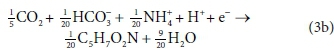
The catabolic half reactions are:

Electron donor:

Electron acceptor:

The overall stoichiometric reaction for catabolism with acetate as the energy source is:

 

Equations 3a, 3b, 4a and 4b are taken from tables of half-reactions for various biological transformations provided by McCarty (1975) and Henze et al. (2008). Each half-reaction is normalized to the 'exchangeable' redox electrons to facilitate the construction of the overall balances.

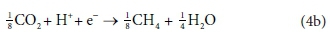
The anabolic and catabolic reactions are then combined as a linear combination into an overall reaction in proportions set by an empirical yield coefficient which expresses the fraction of substrate chemical oxygen demand (COD) that becomes biomass COD.

The result is a stoichiometric reaction equation which satisfies the complete set of elemental balances and the electron balance.

Assigning the empirical stoichiometric formula (C₅H₇O₂N) to represent the biomass is a key step in this development, as it provides the link to the precise stoichiometry of the inorganic components. Part 2 (Brouckaert et al., 2021) extends the concept to all organic wastewater components, and to additional elements using the empirical formulae C_xH_yO_zN_aP_bS_c^ch for the electron donor and C_kH_lO_mN_nP_pS_s for the biomass. It is also demonstrated how all the relevant summary characteristics like COD can be calculated from such a formula.

This general approach has been followed in many bioprocess models, notably those developed by Ekama and co-authors (e.g. Sötemann et al., 2005a, c; Poinapen and Ekama, 2010a, b; Lu et al., 2012; Brouckaert et al., 2010). For our present purpose we modify the approach in two respects:

• The stoichiometric balances are written in terms of the inorganic speciation model components in order to facilitate the integration of the biological and inorganic sub-models.

•I nstead of building the stoichiometric balances by hand from the relevant redox half-reactions, matrix methods are used to solve for the coefficients of the overall balances.

Reaction stoichiometry

A stoichiometric reaction equation represents a set of charge and element balances. In the integrated approach, the stoichiometric balances are expressed in terms of the pre-determined model components. Thus, with one qualification, the only information required to find the coefficients of a stoichiometric reaction equation are:

• The list of components involved in the reaction.

• The elemental content and the charge of each component.

The qualification concerns the degrees of freedom in the set of balances. The standard case is that if a system involves n balances (e.g. n - 1 elements plus charge), it will involve n + 1 components, and have 1 degree of freedom. The degree of freedom is conventionally taken up by arbitrarily setting the value of one of the stoichiometric coefficients.

For example, consider the degradation of acetic acid to carbon dioxide and methane:

In terms of standard aquatic chemistry components, this is equivalently expressed as:

This list of components has 5 entries: CH₃COO^-, H₂O, CO₃⁼, H⁺ and CH₄.

There are 3 element balances (C, H, and O) and a charge balance (or, equivalently an e⁻ balance).

So there is 1 degree of freedom, which is taken up by fixing the value of any one of the coefficients, e.g., pre-setting the coefficient of CH₄ in Eq. 6b to 1, after which all the remaining coefficients are found by solving the four balance equations.

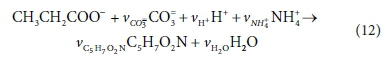
However, consider the reaction equation for acetogenesis (from Sötemann et al., 2005a):

In terms of standard aquatic chemistry components this is expressed as:

Equation 7b involves 6 components and only 4 balances, and therefore has an extra degree of freedom. For this to be a valid stoichiometric reaction (since stoichiometric equations simply represent degrees of freedom in the compositional space), there must be some prior knowledge of the system which takes up the extra degree of freedom. In this case, the ratio of H₂ to CH₃COO^- produced by the reaction was fixed at 3:1. This may have been based on experimental experience, or a characteristic of the biological pathway, or it may merely have been a simplifying assumption - combining two reactions into one. Whatever the reason, the balances cannot be solved without pre-setting an additional coefficient value. In Eq. 7a, the coefficient of CH₃COO^- was set to 1, and that of H₂ to 3, after which all the remaining coefficients were found by solving the balance equations.

Reaction 7 will be used to illustrate the general method of deriving reaction stoichiometry. The elemental content matrix E for the components involved is shown in Table 1.

 

 

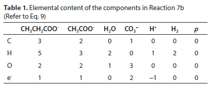
The last row of Table 1 contains the electron balance. This could have been equivalently expressed as a charge balance by simply changing the signs of the entries, e.g., the +2 under the CO₃⁼ means the presence of two e⁻ and the -1 below the H⁺ means the absence of an e⁻.

The coefficients of each component in the reaction that need to be found are placed in a stoichiometric coefficient vector v. Positive coefficient values indicate products (right-hand-side entries) of the reaction, and negative values indicate reactants (left-hand-side entries). Thus for Reaction 7b:

The superscript T in Eq. 6 indicates the transpose of the vector (i.e. v is a column vector)

Then, the stoichiometric balance equations are expressed as the matrix equation:

where ρ signifies the right-hand-side column vector of the equation (a zero vector at this point - the right-most column in Table 1).

Equation 9 has no solution because E is not square (its dimensions are 4 x 6). To obtain a unique solution for the vector v, it has to be augmented by adding 2 rows, corresponding to pre-setting two of the stoichiometric coefficients. For instance, if v_CH3COO^- is set to 1 and v_H2 is set to 3, the augmented matrix E_A is shown in Table 2, in which the last row is equivalent to v_H2 = 3.

 

 

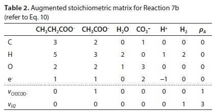
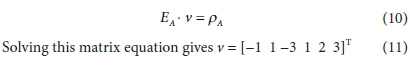
The equation to be solved is then:

Anabolic and catabolic reactions

The distinguishing characteristic of biological reactions is the coupling between anabolic and catabolic reactions. This is usually modelled by introducing a yield coefficient, which represents the fraction of substrate that is consumed by the anabolic reaction. Treating the yield coefficient as an empirical constant is a modelling simplification: in reality it depends on kinetic and equilibrium factors, but in many cases the dependence is not very strong. So, once again, prior knowledge of the system is used to reduce the model's dimensionality, and therefore its complexity.

Obtaining the overall biological reaction stoichiometry is thus simply a matter of obtaining the stoichiometry of the anabolic and catabolic reactions separately according to the method described above, and forming a linear combination in terms of the yield coefficient.

This methodology requires the elemental content of biomass and substrates (electron donors) to be known. It has been common for biochemical models to represent indeterminate organic substances in wastewater purely in terms of their COD, as in ASM1 (Henze et al., 1987). Such a representation is insufficient for modelling physico-chemical processes, and various methods have been used to supply the additional information, such as mass ratios for carbon content (f_C, gC/gCOD), and nitrogen content (f_N, gN/gCOD), which is considered in Part 3 of this series. In the present treatment, we have adopted the use of empirical molecular formulae such as C_xH_yO_zN_aP_bS_c^ch to represent complex organics of unknown structure, and C_kH_lO_mN_nP_pS_s for biomass to distinguish it from the electron donor. With this representation, the method outlined in the previous section can be used without modification to determine the stoichiometric coefficients of the separate anabolic and catabolic reactions. The only stipulation is that the substrate coefficient is always pre-set to -1 in both reactions in order to make the application of the yield coefficient straightforward.

The anabolic reaction for biomass growth on propionate is:

Reworking the derivation according to the matrix method, the augmented stoichiometric matrix is shown in Table 3:

 

 

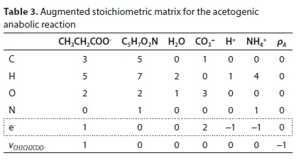
After solving separately for the anabolic and catabolic stoichiometric coefficient vectors (see Table 4), the overall reaction coefficient vector is simply:

 

 

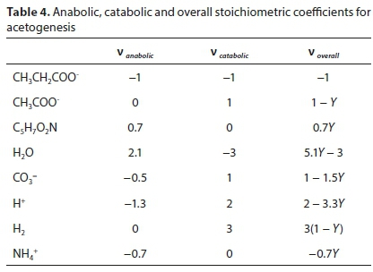
where Y is the yield coefficient.

The set of coefficients obtained according to Eq. 13 are formulated on the basis of 1 mole of substrate consumed. It may be convenient to re-scale it to a different basis to suit the form of its rate expression. A commonly used basis is 1 g of biomass COD produced, as in the ASMs (Henze et al., 2000).

For the acetogenesis example, the catabolic reaction is Reaction 7b. The vector of stoichiometric coefficients needs to be expanded to accommodate both the catabolic and anabolic reactions:

The results are shown in Table 4 using molal units, which depend on the molecular formula used to represent the biomass (C₅H₇O₂N). The COD per mol of the biomass formula is 223.986 g O₂/mol, so converting to a basis of 1g COD of biomass produced involves dividing all the terms of v_overall by 223.986 × 0.7Y.

Note that the yield coefficient Y in this case has the same numerical value irrespective of the units used, since it is defined as the fraction of substrate consumed which goes to the anabolic reaction. This is the same whether expressed in terms of moles, grams or COD of substrate. This does not apply to all biochemical processes, e.g., for autotrophic nitrification the conventional definition of the yield coefficient expresses biomass COD produced per N removed, and the numerical value does depend on the units used.

This methodology is fundamentally the same as set out by McCarty (1975). However, it does not employ two prominent devices that he presented: the concept of the exchangeable electrons of each component, and the division of each reaction into oxidation and reduction half-reactions. In fact, these are not essential features of his method; they are just aids for avoiding errors when determining the coefficients by hand. The use of symbolic algebraic software makes these aids dispensable. However, McCarty's exchangeable electron concept remains an important aid to an understanding of the reaction system.

Exchangeable electrons / electron donating capacity / COD

As pointed out by McCarty (1975), COD expresses the electron donating capacity of a substance as the mass of oxygen which could take up the electrons, i.e., 8g O /mol electrons in the COD test (discussed further in Part 2, Brouckaert et al., 2021). This information is actually inherent in the elemental content matrix. If we consider a generic reaction in which one organic component is transformed into another:

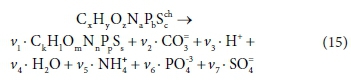
The elemental content matrix for this reaction is shown in Table 5:

This is a 7 x 8 matrix, and consequently has no determinant. If the column for the product biomass C_kH_lO_mN_nP_pS_s is deleted (i.e. only the catabolic reaction is considered), the remaining matrix is 7 x 7, and its determinant is:

Similarly, if the column for the substrate C_xH_yO_zN_aP_bS_c^ch is deleted, the determinant of the remaining matrix is:

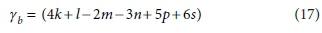
The composite stoichiometric factors γ_s and γ_b are identical to the exchangeable electrons of the organic components in the McCarty (1975) treatment. When one solves the matrix equation (Eq. 10) for the stoichiometric coefficients, γ_s and γ_b appear as factors in the solution. One can also derive the forms of γ_s and γ_b by considering the changes taking place in oxidation states of the elements in the organic component during the reaction, which is how McCarty arrived at them.

This demonstrates the equivalence of the elemental matrix and the electron balancing methods for deriving the stoichiometric coefficient values. However, keeping track of the electrons through a complex set of reactions often provides insight into the mechanisms involved, which is difficult to obtain just by inspecting the elemental matrix. Note that for reasons discussed in Part 2, the term 'exchanged electrons of reaction' is preferred to the term 'exchangeable electrons'. The electrons donated and accepted by the various organic and inorganic components in various biochemical processes are discussed in greater detail in Part 2 (Brouckaert et al., 2021).

Stoichiometric balances and speciation

As discussed in the previous sections, biological stoichiometric reactions are simply material balances which keep track of the elemental and electron content of the products and reactants in biological transformations. They generally do not predict changes in speciation resulting from biological transformations or the distribution of species between phases.

Comparing Eqs 6a with 6b and 4c, and 7a with 7b, it is clear that the same stoichiometric reaction can be written it terms of several different sets of components and still be balanced overall. Our recommendation is that the stoichiometric equations should always be set up in terms of the standard aquatic chemistry modelling components as discussed in the previous sections. However, in other modelling approaches, there is some freedom to choose which components to include in the biological stoichiometric balances.

For example, McCarty (1975) tended to set up his half-reactions in terms of the transfer of one mole of protons plus one mole of electrons (H⁺ + e⁻ in Eqs 3 and 4). In many cases, this leads to half-reactions expressed in terms of two different carbonate species, as, for example, in Eq. 4a:

This does not necessarily mean that one mole of acetate will produce one mole of CO₂ and one mole of HCO₃^-. The actual distribution of carbonate species will depend on the entire ionic composition, which also determines properties such as the pH.

In terms of standard aquatic chemistry components, this is equivalent to:

In Eq. 18, the component CO₃⁼ represents the sum of all the carbonate species produced (including any gaseous CO₂ evolved). Once the composition of the solution has been determined by flow and reaction balances in terms of concentrations of components, the speciation calculation can be employed to determine the concentrations of equilibrium species. So, for example, the total CO₃⁼ concentration (component concentration, as referred to in Eq. 18) would be calculated by material balance. The carbonate species concentrations, such as [H₂CO₃], [HCO₃⁻] and [CO₃²⁻], are then determined from the speciation calculation. Therefore, standard chemical notation can be confusing, since, apart from the typeface, the same symbol CO₃⁼ in this paragraph refers to both a component and a species, which are conceptually quite different. However, the context makes it clear whether a component or species is being referred to. In a dynamic model, with kinetic and equilibrium parts, both sets of calculations have to be carried out at each integration time step, because reaction rates and phase separations generally depend on species concentrations rather than component concentrations. So the stoichiometric mass-balanced time-dependent differential equations part is solved for the changes in component concentrations and the equilibrium speciation algebraic equations part of the model speciates the new component concentrations into species concentrations. These issues will be further discussed in Part 5 of this series.

 

ALKALINITY

It is usually impractical to define the complete ionic composition of a wastewater aqueous phase, because there are too many possible dissolved components that can be present. Alkalinity, or proton accepting capacity (PAC), is a summary property, easily measured by titration, which provides important information about how biological processes interact with the aqueous environment in which they take place. Part 4 of this series discusses alkalinity further from the measurement point of view, and Part 5 looks at the computational aspects; but for the present purpose, the alkalinity of the aqueous phase is the remaining capacity of the weak-acid anions (e.g. HCO₃^-) present in it to bind protons (e.g. HCO₃^- becoming H₂CO₃), thereby reducing the free proton (H⁺) concentration, and so acting against a decrease in pH when acid is added (imparting buffer capacity). At the titration end-point, which for the H₂CO₃ alkalinity is in the vicinity of pH 4.5 (see Part 4 or Loewenthal et al., 1989), the H₂CO₃ alkalinity is, by definition, zero relative to the selected reference species for the alkalinity, in this case H₂CO₃. In 'natural' waters, alkalinity principally is provided by the inorganic carbon (IC) anions. However, in wastewaters additional contributions are made by other weak-acid species such as acetate, ammonia (NH₃, propionate, ortho-phosphate (OP) and sulphide (FSS, HS⁻). Since biological redox reactions can either take up or produce these anions, as well as protons, they cause changes in the aqueous alkalinity and pH which are important to understand in systems where pH affects the bioprocess rates, such as those of acetoclastic methanogenesis or BSR in AD.

Alkalinity is usually expressed units of mg/L as CaCO₃ . For the present purpose it is more useful to use units of mol H⁺/L, where mol H⁺/L x 50 000 yields mg/L as CaCO₃ (Loewenthal and Marais, 1976). Alkalinity arises from the formation of protonated species in solution. However, it can also be expressed in terms of component concentrations (Snoeyink and Jenkins, 1980). It is this aspect which is relevant to Parts 1 and 2 of this series.

To illustrate how alkalinity is related to components, consider a solution that is made up of Na₂CO₃, Na₃PO₄, NaAc and NaHS in pure water. These are the sodium salts of the weak-acid anions that commonly contribute to alkalinity, which means that they tend to bind H⁺ in aqueous solution to form the protonated species HCO₃⁻, H₂CO₃, HPO₄²⁻, H₂PO₄⁻, H₃PO₄, HAc, H₂S and HS⁻. The salts that the solution of the example was made from contain no H⁺. (The H in NaHS is bound to S as HS^-). When protonated to the maximum extent possible, their weak-acid anions will be entirely converted to H₂CO₃, H₃PO₄, HAc, and H₂S, which are defined to be the alkalinity reference species.

So the capacity of the initial solution to bind H⁺ (its alkalinity) is given by:

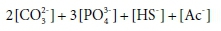
where […] indicates a component concentration in mol/kg.

As [H⁺] is added to the solution by titrating with a strong acid such as HCl, the added H⁺ progressively reduces the solution's capacity to bind further H⁺, that is, it reduces the alkalinity. Hence the alkalinity of the solution during the course of the titration is given by:

In the measurement context, the alkalinity is defined by the titration with strong acid, which will be affected in various ways by the presence of acid and base species in the original solution. The pH of the example solution is about 11, and if 0.001 M NH₄Cl is added to it, the NH₄⁺ will give up most of its H⁺ as it dissolves, to bind with the weak-acid anions in the solution, forming NH_3(aq). This exchange will have some effect on the speciation of the solution, and consequently the pH and the distribution of alkalinity among the components, but no effect on the total alkalinity. In terms of measurement, this is manifested as a change in the shape of the pH titration curve, but no change in the total acid required to reach the titration endpoint, where the NH_3(aq) will essentially have been all converted back to NH₄⁺. In terms of components, it is explained by saying that NH₄⁺ is the reference species for alkalinity, so adding NH₄⁺ does not affect Alk_T, so Eq. 19a is unchanged (Loewenthal et al., 1991).

Adding a strong base, such as NaOH (sodium hydroxide), will increase the total acid required to titrate to the endpoint, and therefore the alkalinity, whereas adding a strong acid such H₂SO₄ or HCl will decrease it. In the case of a strong acid, the effect on Eq. 19a can be made explicit by noting that in solution strong acids are present in their fully dissociated forms:

Expressing strong acids in their dissociated form is useful for avoiding confusion in the stoichiometric manipulations that are discussed in Part 2 (Brouckaert et al., 2021). The strong base case is less obvious, as OH⁻ is not one of the standard aquatic chemistry components: where required, it is represented as (H₂O - H⁺). However, H₂O is usually modelled as an invariant background component, and not represented explicitly. Thus OH⁻ is effectively (-H⁺), which means that is already accounted for in Eq. 19a.

Sulphide involves a similar issue. The standard component representing sulphides is HS⁻, not S²⁻, which is considered virtually non-existent as an aqueous solution species. So, if the NaHS in our solution example is replaced by Na₂S, the S²⁻ is represented as (HS⁻- H⁺). Once again, Eq. 19a is unchanged, but the [H⁺] term includes a negative contribution from the sulphide.

So far, the discussion has assumed that the total alkalinity becomes zero when all the relevant acid anions are fully protonated. The limiting species for achieving this condition is H₃PO₄, which is a strong acid, only approaching full protonation at very low pH < 1 (although H₂PO₄⁻ and HPO₄²⁻ are weak acids). All the other components are fully protonated around pH 4. By a fortunate coincidence, the titration endpoint for H₂PO₄⁻ is also around pH 4. So for measurement purposes it is convenient to take the reference species for phosphate as H₂PO₄⁻ rather than H₃PO₄ (Loewenthal et al., 1989). Thus there are two versions of total alkalinity in use, H₂CO₃ / H₃PO₄ / NH₄⁺ / H₂S / HAc alkalinity, which we indicate by Alk_T, and H₂CO₃ / H₂PO₄⁻ / NH₄⁺ / H₂S / HAc alkalinity, which we will indicate as Alk_t.

Comparing Eqs 19a and 19b, the difference between the two alkalinity versions is simply:

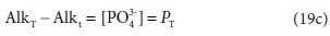
where P_T is the total ortho-phosphate concentration.

Equations 19a to 19c are written in terms of standard aquatic chemistry components, which is fundamentally an arbitrary choice. There are situations where it is convenient to represent systems in terms of different sets of components. For instance, the composition of our example solution could be expressed in terms of HCO₃^- and HPO₄²⁻, instead of CO₃²⁻ and PO₄³⁻ In this case, Eqs 19a and 19b are replaced by:

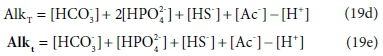
In Eqs 19d and 19e, [HCO₃^-] and [HPO₄²⁻] have the same values as [CO₃²⁻] and [PO₄³⁻] in Eq. 19a and 19b, but the value of [H⁺] is reduced to account for the H⁺ content of the substituted components.

Total alkalinity change of reaction

Since the total alkalinity of a solution can be expressed as a linear combination of component quantities, it is also a conserved stoichiometric property of the solution, and so can be used, for example, in mixing calculations (Loewenthal et al., 1989, 1991). Chemical reactions which produce or consume weak acids or bases and protons will change the alkalinity of the aqueous phase, and the change that occurs is a stoichiometric property of the reaction. In the same way that the enthalpy change or exchanged electrons of reaction (Part 2, Brouckaert et al., 2021) are used in energy and electron balances for reacting systems, the concept of total alkalinity change of reaction allows alkalinity balances for reacting systems.

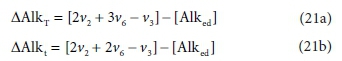
The total alkalinity change of reaction is calculated from the difference between the coefficients of the component products and those of the component reactants relevant to the alkalinity, with respect to the selected reference species, i.e.:

For Eq. 15 the product components contributing to the ∆Alk_T of the reaction are +v₂CO₃²⁻, +v₆PO₄³⁻ and -v₃ H⁺. If the generic reactant component C_xH_yO_zN_aP_bS_c^ch is a weak acid/base component itself that contributes to alkalinity, such as NH₃, HS^- or CH₃COO^-, then its consumption by the reaction contributes to the alkalinity change of the reaction. However, if the generic component is a strong acid/base anion or cation such as S₂O₃^2-, or an insoluble or an uncharged organic, such as particulate starch, urea or dissolved glucose, then it does not contribute. This means that the nature of the generic reactant component needs to be known and the reference species for the alkalinity defined to know whether or not it contributes to the ∆Alk_T of the reaction. Following Eqs 19a and 20 for the ∆Alk_T of Eq. 15 yields Eq. 21, where the alkalinity of the electron donor (Alk_ed) is 0 if the generic component does not contribute to the alkalinity of the reactants, or 1, 2 or 3 if it does and is 1, 2 or 3 dissociations away from the reference species.

These distinctions reduce the utility of the generalized Eq. 21, because one has to know what the generalized component is to select the correct value for Alk_ed. The issue is that, although alkalinity is a stoichiometric quantity, unlike all the other stoichiometric quantities considered in this series of papers, the alkalinity contribution of a component is not determined solely by its elemental make-up.

Direct, latent and persistent alkalinity

If sodium acetate (NaAc NaC₂H₃O₂ Na⁺ + C₂H₃O₂⁻) is added to a solution, the acetate adds 1 mol of alkalinity per mol acetate to the solution (Alk_T or Alk_t). If it is subsequently oxidised to carbonate (C₂H₂O₂⁻ + 2O₂ → 2CO₃²⁻ + 3H⁺) the acetate alkalinity is transformed to carbonate alkalinity, to the extent of (2 x 2 - 3 = 1) mol alkalinity per mol acetate that was added. This phenomenon can be described as the electron donor, acetate, having direct alkalinity (∆Alk_ed) and persistent alkalinity (Alk_p), which persists in the solution after the acetate is removed by the reaction. Although Alk_ed is a true property of the component, the persistent alkalinity depends on the products of the reaction and is therefore a property of the reaction. Nevertheless, in a given redox environment, it can be useful to think of it as a quasi-property of the component.

In the above example, the direct and persistent alkalinities of the acetate both have the same value, since ∆Alk_T for the reaction is zero; however, this is not always the case. Consider the oxidation of urea: (NH₂CONH₂ + 4O₂ → CO₃²⁻ + 4H⁺ + 2NO₃⁻). Urea is uncharged, so has no direct alkalinity (Alk_ed = 0). However, ∆Alk_T for the reaction is (2 - 4 - 0 - 4 x 0 = -2), so the persistent alkalinity of urea, when its elements are all completely oxidized, is -2 mol/mol; adding urea to the solution will initially have no effect on its alkalinity, but will reduce it as the oxidation reaction proceeds. In a different redox environment, such as an anaerobic reactor, the N reaction product could be NH₄⁺ rather than NO₃⁻, in which case the reaction is NH₂CONH₂ + H₂O → CO₃²⁻ + 2NH₄⁺. In this case ∆Alk_T = 2 + 2 x 0 - 0 - 0 = +2 mol/mol.

From the above, all the alkalinity in the aqueous phase produced by reaction Eq. 15 comes from the electron donor C_xH_yO_zN_aP_bS_c^ch relative to the reaction products. So the ∆Alk_T can be described as latent alkalinity stored in the electron donor, and released to the aqueous phase during the redox reaction. Thus the persistent alkalinity of the electron donor is given by:

The additional alkalinity is therefore not 'created' by the reaction - it is latent in the electron donor, and released to the aqueous phase by the reaction. If the e⁻ donor is dissolved, then the direct alkalinity of the e⁻ donor is also in the aqueous phase and the reaction adds the latent alkalinity from the reactant component. Furthermore, a reaction that produces biomass takes up alkalinity and stores it in a particulate form, external to the aqueous phase, although in contact with it. Via this mechanism, alkalinity is commonly transferred from the aqueous phase in an activated sludge reactor, where heterotrophic biomass is produced, to an anaerobic digester, where the alkalinity reappears in the aqueous phase at very high concentration after digestion, because the waste activated sludge (WAS) biomass is thickened before AD (Part 2, Brouckaert et al., 2021). However, since the redox environments are different, the alkalinity released anaerobically may differ from the alkalinity stored aerobically - it depends on the other components involved in the respective reactions.

 

CONCLUSIONS

The concepts and methods presented are part of a pragmatic framework for modelling wastewater treatment processes that reflects the current state of knowledge. The completely rigorous approach to chemical reactions involves conservation of matter (stoichiometry), conservation of energy, equilibria and kinetics. Every process is governed by all these factors. However, in many cases models can be simplified by neglecting aspects which are not limiting. Such a simplification applies, not only to the mathematical formulation of models, but also to the experimental methods for obtaining the data required to support the modelling. Thus, most models and measurement techniques associated with wastewater treatment reflect the fact that the biochemical reactions tend to be limited by stoichiometric and kinetic factors. On the other hand, inorganic aqueous models and measurements tend to reflect stoichiometric and equilibrium limitations. When a model needs to represent the interaction between the biochemical reactions and the inorganic reactions, the experimental effort to obtain complete thermodynamic and kinetic data for all the components involved would be enormous, particularly since the exact natures of most organic components are unknown. Retaining the main simplifications that have commonly been applied in both biochemical and inorganic chemistry models makes the task of integrating them manageable.

Nevertheless, it is important to be aware of the rigorous picture, so as to ensure that any simplifications made are appropriate, and to understand their limitations. So, for example, it was pointed out in the section on anabolic and catabolic reactions that a yield coefficient represents a stoichiometric approximation to a thermodynamic limitation. Experience has shown that the approximation is good in many practical circumstances, because yield coefficients do not vary excessively within the range of conditions commonly encountered in wastewater treatment. On the other hand, the speciation of weak acids and bases is much more variable, and for this a stoichiometric approximation will only be appropriate in a very narrow pH range. Fortunately, the modelling tools that we present allow us to construct models that do not resort to such speciation approximations.

 

ABBREVIATIONS

AD anaerobic digestion

ADM1 Anaerobic Digestion Model 1

AS activated sludge

ASM activated sludge models

COD chemical oxygen demand

OP ortho phosphate

 

SYMBOLS

Alk_ed direct alkalinity of the electron donor component

Alk_p persistent alkalinity of the electron donor component (Alk_ed + ∆Alk_T)

Alk_T total alkalinity in solution

∆Alk_T total alkalinity change of reaction

a molar content of nitrogen in C_xH_yO_zN_aP_bS_c^ch electron donor

b molar content of phosphorus in C_xH_yO_zN_aP_bS_c^ch electron donor

c molar content of sulphur in C_xH_yO_zN_aP_bS_c^ch electron donor

ch charge of C_xH_yO_zN_aP_bS_c^ch electron donor

C_xH_yO_zN_aP_bS_c^ch generalized electron donor formula

C_kH_lO_mN_nP_pS_s generalized biomass formula

E elemental content matrix

E_A augmented elemental content matrix

l molar content of hydrogen in C_kH_lO_mN_nP_pS_s biomass

m molar content of oxygen in C_kH_lO_mN_nP_pS_s biomass

n molar content of nitrogen in C_kH_lO_mN_nP_pS_s biomass

p molar content of phosphorus in C_kH_lO_mN_nP_pS_s biomass

s molar content of sulphur in C_kH_lO_mN_nP_pS_s biomass

x molar content of carbon in C_xH_yO_zN_aP_bS_c^ch electron donor

y molar content of hydrogen in C_xH_yO_zN_aP_bS_c^ch electron donor

Y biomass yield coefficient

z molar content of oxygen in C_xH_yO_zN_aP_bS_c^ch electron donor

γ_b exchangeable electrons of biomass

γ_s exchangeable electrons of the electron donor

v stoichiometric coefficient vector

ρ vector of right-hand-side terms of the element balance equations

 

REFERENCES

ALLISON JD, BROWN DS and NOVO-GRADAC KJ (2009) MINTEQA2. URL: http://www.epa.gov/ceampubl/mmedia/minteq/ (Accessed 8 Dec 2009).         [ Links ]

ANDREWS JF and GRAEF SP (1971) Dynamic modelling of the anaerobic digestion process. Anaerobic Biological Treatment Processes. Advances in Chemistry Series No. 105. American Chemical Society, Washington D.C. 126-162. https://doi.org/10.1021/ba-1971-0105.ch008        [ Links ]

BARAT R, MONTOYA T, SECO A and FERRER J (2011) Modelling biological and chemically induced precipitation of calcium phosphate in enhanced biological phosphorus removal systems. Water Res. 45 3744-3752. https://doi.org/10.1016/j.watres.2011.04.028        [ Links ]

BATSTONE DJ, KELLER J, ANGELIDAKI I, KALYUZHNYI SV, PAVLOSTATHIS SG, ROZZI A, SANDERS WTM, SIEGRIST H and VAVILIN VA (2002) Anaerobic digestion model No 1 (ADM1). Scientific and Technical Report No. 13. International Water Association (IWA), London. https://doi.org/10.2166/wst.2002.0292        [ Links ]

BATSTONE DJ, AMERLINCK Y, EKAMA G, GOEL R, GRAU P, JOHNSON B, KAYA I, STEYER J-P, TAIT S, TAKÁCS I, VANROLLEGHEM PA, BROUCKAERT CJ and VOLKE E (2012) Towards a generalized physicochemical framework. Water Sci. Technol. 66 (6) 1147-1161. https://doi.org/10.2166/wst.2012.300        [ Links ]

BROUCKAERT CJ, IKUMI DS and EKAMA GA (2010) A 3 phase anaerobic digestion model. In: Proceedings of the 12^th IWA Anaerobic Digestion Conference (AD12), 1-4 November 2010, Guadalajara, Mexico.         [ Links ]

BROUCKAERT CJ, EKAMA GA, BROUCKAERT BM and IKUMI DS (2021) Integration of complete elemental mass balanced stoichiometry and aqueous phase chemistry for bioprocess modelling of liquid and solid waste treatment systems - Part 2: Bioprocess stoichiometry. Water SA. 47 (3) 289-308.         [ Links ]

DOLD PL, EKAMA GA and MARAIS GvR (1980) A general model for the activated sludge process. Progr. Water Technol. 12 (6) 47-77. https://doi.org/10.1016/B978-1-4832-8438-5.50010-8        [ Links ]

EKAMA GA (2009) Using bio-process stoichiometry to build a plant-wide mass balance based steady-state WWTP model. Water Res. 43 (8) 2101-2120. https://doi.org/10.1016/j.watres.2009.01.036        [ Links ]

FIDALEO M and LAVECCHIA R (2003) Kinetic study of urea hydrolysis in the pH range 4-9. Chem. Biochem. Eng. Q. 17 (4) 311-318.         [ Links ]

GRAU P, DE GRACIA M, VANROLLEGHEM PA and AYESA E (2007) A new plant wide methodology for WWTPs. Water Res. 41 (19) 4357-4372. https://doi.org/10.1016/j.watres.2007.06.019        [ Links ]

HENZE M, GRADY CPL Jnr, GUJER W, MARAIS GVR and MATSUO T (1987) Activated Sludge Model No 1. IWA Scientific and Technical Report No 1. International Water Association (IWA), London. https://doi.org/10.2166/9781780401867        [ Links ]

HENZE M, GUJER W, MINO T and VAN LOOSDRECHT M (2000) Activated Sludge Models ASM1, ASM2, ASM2d, and ASM3. IWA Scientific and Technical Report No 9. International Water Association (IWA), London.         [ Links ]

HENZE M, VAN LOOSDRECHT MCM, EKAMA GA and BRDJANOVIC D (2008) Biological Wastewater Treatment: Principles, Modelling and Design. IWA Publishing, London. 528 pp.         [ Links ]

IKUMI DS, BROUCKAERT CJ and EKAMA GA (2011) A 3 phase anaerobic digestion model. 8^th IWA Watermatex conference, San Sebastian, Spain, 20-22 June 2011.         [ Links ]

IKUMI DS, HARDING TH, BROUCKAERT CJ and EKAMA GA (2014) Plant wide integrated biological, chemical and physical processes modelling of wastewater treatment plants in three phases (aqueous-gas-solid). PhD thesis, Research Report W138, Department of Civil Engineering, University of Cape Town, Rondebosch, 7700, South Africa.         [ Links ]

IKUMI DS, HARDING TH, VOGTS M, LAKAY MT, MAFUNGWA HZ, BROUCKAERT CJ and EKAMA GA (2015) Mass balances modelling over wastewater treatment plants III. WRC Report No. 1822/1/14. Water Research Commission, Pretoria. ISBN 978-1-4312-0614-8.         [ Links ]

LIZZARALDE I, FERNANDEZ-AREVALO T, BROUCKAERT CJ, VANROLLEGHEM P, IKUMI DS, EKAMA GA, AYESA E and GRAU P (2015) A new general methodology for incorporating physico-chemical transformations into multiphase wastewater treatment process models. Water Res. 74 239-256. https://doi.org/10.1016/j.watres.2015.01.031        [ Links ]

LOEWENTHAL RE and MARAIS GvR (1976) Carbonate chemistry of aquatic systems - theory and application. Ann Arbor Science Publishers, Ann Arbor, MI. Library of Congress 76-24963, ISBN 0-25040141-X.         [ Links ]

LOEWENTHAL RE, EKAMA GA and MARAIS GvR (1989) Mixed weak acid/base systems Part I - Mixture characterization. Water SA. 15 (1) 3-24.         [ Links ]

LOEWENTHAL RE, WENTZEL MC, EKAMA GA and MARAIS GvR (1991) Mixed weak acid/base systems Part II: Dosing estimation, aqueous phase. Water SA. 17 (2) 107-122.         [ Links ]

LU H, EKAMA GA, WU D, FENG J, VAN LOOSDRECHT MCM and CHEN GH (2012) SANI process realizes sustainable saline sewage treatment: Steady state model-based evaluation of the pilot-scale trial of the process. Water Res. 46 (2) 475-490. https://doi.org/10.1016/j.watres.2011.11.031        [ Links ]

MCCARTY PL (1975) Stoichiometry of biological reactions. Prog. Water Tech. 7 (1) 157-172.         [ Links ]

MUSVOTO EV, WENTZEL MC, LOEWENTHAL MC and EKAMA GA (2000a) Integrated chemical-physical processes modelling - I. Development of a kinetic-based model for mixed weak acid/base systems. Water Res. 34 (6) 1857-1867. https://doi.org/10.1016/S0043-1354(99)00334-6        [ Links ]

MUSVOTO EV, WENTZEL MC and EKAMA GA (2000b) Integrated chemical-physical processes modelling - II. Simulating aeration treatment of anaerobic digester supernatants. Water Res. 34 (6) 1868-1880. https://doi.org/10.1016/S0043-1354(99)00335-8        [ Links ]

PARKHURST DL and APPELO CAJ (2013) PHREEQC (Version 3). A computer program for speciation, batch-reaction, one-dimensional transport, and inverse geochemical calculations. URL: ftp://brrftp.cr.usgs.gov/pub/charlton/phreeqc/Phreeqc_3_2013_manual.pdf (Accessed 19 November 2013). https://doi.org/10.3133/tm6A43        [ Links ]

POINAPEN J and EKAMA GA (2010a) Biological sulphate reduction with primary sewage sludge in an up flow anaerobic sludge bed reactor - Part 5: Steady-state model. Water SA. 36 (3) 193-202.         [ Links ]

POINAPEN J and EKAMA GA (2010b) Biological sulphate reduction with primary sewage sludge in an up flow anaerobic sludge bed reactor - Part 6: Development of a kinetic model for BSR. Water SA. 36 (3) 203-214.         [ Links ]

SERRALTA J, FERRER J, BORRAS L and SECO A (2004) An extension of ASM2d including pH calculation. Water Res. 38 (19) 4029-4038. https://doi.org/10.1016/j.watres.2004.07.009        [ Links ]

SMITH JM and VAN NESS HC (2005) Introduction to Chemical Engineering Thermodynamics (7^th edn). McGraw Hill, New York.         [ Links ]

SNOEYINK VL and JENKINS D (1980) Water Chemistry. John Wiley and Sons, New York.         [ Links ]

SOLON K, FLORES-ALSINA X, KAZADI MBAMBA C, VOLKE EIP, TAIT S, BATSTONE D, GERNAEY KV and JEPPSON U (2015) Effects of ionic strength and ion pairing on (plant-wide) modelling of anaerobic digestion. Water Res. 70 235-245. https://doi.org/10.1016/j.watres.2014.11.035        [ Links ]

SÖTEMANN SWN, VAN RENSBURG P, RISTOW NE, WENTZEL MC, LOEWENTHAL RE and EKAMA GA (2005a) Integrated chemical/physical and biological processes modelling Part 2 - Anaerobic digestion of sewage sludges. Water SA. 31 (4) 545-568. https://doi.org/10.4314/wsa.v31i4.5145        [ Links ]

SÖTEMANN SW, RISTOW NE, WENTZEL MC and EKAMA GA (2005b) A steady-state model for anaerobic digestion of sewage sludges. Water SA. 31 (4) 511-527. https://doi.org/10.4314/wsa.v31i4.5143        [ Links ]

SÖTEMANN SW, MUSVOTO EV, WENTZEL MC and EKAMA GA (2005c) Integrated chemical, physical and biological processes kinetic modelling Part 1 - Anoxic and aerobic processes of carbon and nitrogen removal in the activated sludge system. Water SA. 31 (4) 529-544. https://doi.org/10.4314/wsa.v31i4.5144        [ Links ]

SPEECE RE (2008) Anaerobic biotechnology and odor/corrosion control for municipalities and industries. Archea Press, Nashville. TN. ISBN 1-57843-052-9. 586 pp.         [ Links ]

STUMM W and MORGAN JJ (1996) Aquatic Chemistry: Chemical Equilibria and Rates in Natural Waters. John Wiley and Sons, New York.         [ Links ]

TAKÁCS I and VANROLLEGHEM PA (2006) Elemental balances in activated sludge modelling. In: Proceedings of the IWA World Water Congress, 10-14 September 2006, Beijing, China.         [ Links ]

WRC (Water Research Commission) (1984) Theory, design and operation of nutrient removal activated sludge processes. Wiechers HNS (Ed.). WRC Report No. TT16/84. Water Research Commission, Pretoria. ISBN 0 908356 13 7.         [ Links ]

 

 

Correspondence:
CJ Brouckaert
Email brouckae@ukzn.ac.za

Received: 13 July 2015
Accepted: 7 July 2021

 

 

APPENDIX

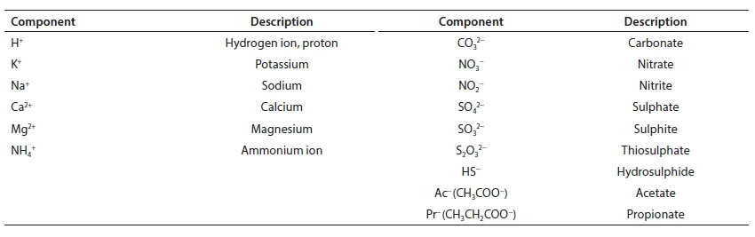
Standard aquatic chemistry components

Reference is made in several places to the set of standard aquatic chemistry components. These are those used by several freely available and widely used aquatic chemistry models, such as MINTEQA2, PHREEQC and Visual MINTEQ. The following table lists the subset of standard components that feature in the series of papers.

 

Click to enlarge