


Servicios Personalizados
Articulo
 Inglés (pdf)
 Articulo en XML
 Referencias del artículo
Indicadores

Links relacionados
-
 Citado por Google
 -
 Similares en Google
Compartir

 Permalink
Water SA
versión On-line ISSN 1816-7950
versión impresa ISSN 0378-4738
Water SA vol.47 no.1 Pretoria ene. 2021
http://dx.doi.org/10.17159/wsa/2021.v47.i1.9444
RESEARCH PAPER
River water quality management using a fuzzy optimization model and the NSFWQI Index
Mohammad Kazem GhorbaniI; Abbas AfsharI; Hossein HamidifarII
ISchool of Civil Engineering, Iran University of Science and Technology, Tehran, Iran
IIWaterEngineering Department, Shiraz University, Shiraz, Iran
ABSTRACT
In this study, a novel multiple-pollutant waste load allocation (WLA) model for a river system is presented based on the National Sanitation Foundation Water Quality Index (NSFWQI). This study aims to determine the value of the quality index as the objective function integrated into the fuzzy set theory so that it could decrease the uncertainties associated with water quality goals as well as specify the river's water quality status rapidly. The simulation-optimization (S-O) approach is used for solving the proposed model. The QUAL2K model is used for simulating water quality in different parts of the river system and ant colony optimization (ACO) algorithm is applied as an optimizer of the model. The model performance was examined on a hypothetical river system with a length of 30 km and 17 checkpoints. The results show that for a given number of both the simulator model runs and the artificial ants, the maximum objective function will be obtained when the regulatory parameter of the ACO algorithm (i.e., q0) is considered equal to 0.6 and 0.7 (instead of 0.8 and 0.9). Also, the results do not depend on the exponent of the membership function (i.e., y). Furthermore, the proposed methodology can find optimum solutions in a shorter time.
Keywords: ACO algorithm, fuzzy set theory, multiple pollutant, NSFWQI, QUAL2K model, waste load allocation model
INTRODUCTION
Many rivers around the world carry significant amounts of pollutants produced by domestic, agricultural, and industrial activities (Farzadkhoo et al. 2018, 2019; Hamidifar et al. 2015). To date, many waste load allocation (WLA) models have been proposed for water quality management in a river system. In general, the purpose of these models is to obtain technically and economically feasible solutions for the pollution control agency (PCA) and dischargers. Organizations set standards and regulations for water use, whereby dischargers are required to remove a percentage of various wastewater pollutants. On the other hand, increasing the fractional removal level of pollutants increases the cost of wastewater treatment. Therefore, trade-offs between conflicting goals between organizations and dischargers have always been a challenge. Many studies have been conducted in the field of water quality management in river systems, each of which has specific characteristics and goals. Mahjouri and Abbasi (2015) attempted to minimize the total cost of wastewater treatment by considering the optimal treatment alternatives and the objectives of the stakeholders. Nikoo et al. (2016) developed a WLA model for a river and applied the policy of allocating total profits from the permitted trade of wastewater discharge among dischargers. Tavakoli et al. (2015) studied the effects ofWLA and wastewater load on river water quality management concerning agricultural water return. Estalaki et al. (2015) proposed appropriate penalty functions to comply with the standards imposed by PCA's water quality standard to dischargers. Ashtiani et al. (2015) and Saberi and Niksokhan (2017) optimized the degree of deviation or deviation from water quality standards in different parts of the river, which is one of the water quality management policies in rivers.
Fuzzy rules and concepts are used to reduce uncertainty in WLA models in the river system. There are various techniques in the fuzzy environment for solving water quality problems. Sasikumar and Mujumdar (1998) mathematically quantified the uncertainties related to vagueness in describing the qualitative goals and reducing water pollution and expressed it in a fuzzy framework, and so used the concepts of fuzzy set theory and its relations to the real sets. Karmakar and Mujumdar (2006) used the concept of gray fuzzy to develop their proposed model for water quality management. Qin et al. (2009) proposed an interval-parameter WLA model for river water quality management under uncertainty. Nikoo et al. (2016) simulated a pollutant charge allocation model and used a fuzzy interval solution. Xu et al. (2017) applied the fuzzy random environment approach to assess river pollution under uncertainty conditions. In some studies, the determination of the concentration of water quality parameters (WQPs) (e.g., either BOD or DO concentration or both) has been considered as an indicator of water quality assessment in the river (Takyi and Lence, 1996; Saadatpour and Afshar, 2007; Lei et al., 2015). However, in others, more than two quality parameters have been investigated (Mahjouri and Abbasi, 2015). Furthermore, in some models, some effective quality parameters are expressed as a separate and standard quality index and are considered as a criterion for water quality assessment (Kannel et al., 2007).
In this study, the National Sanitation Foundation Water Quality Index (NSFWQI) is used to determine the water quality in a river system. This popular index determines water quality using 9 effective quality parameters of environmental water. To reduce some uncertainties in the proposed model, the fuzzy set theory has been applied expansively. The objectives of this model are to consider the optimal water quality in the river for the stakeholders so that the costs of the wastewater treatment plants remain acceptable. Another new approach applied here is to optimize the fuzzy objective function in the form of the average NSFWQI quality index at the river checkpoints. The advantage of using the NSFWQI as the membership function in the proposed model is that it considers the uncertainties related to the WLA model and also can generate a set of more accurate solutions.
To simulate and optimize the river water quality model, the QUAL2K simulator and ant colony optimization (ACO) algorithm are used simultaneously to determine the appropriate solutions of the model, and thus to increase the speed and accuracy in the determination of model solutions. The model is run on a hypothetical river and the results are analysed. The model results can contribute to faster and more accurate decisions.
Water quality index (WQI)
One of the known indices that are used for determining water quality is the NSFWQI, which was provided by Brown et al. (1970) and was supported by the National Sanitation Foundation of the United States. For this reason, Brown's index is also referred to as NSFWQI. This index is scaled from 0 to 100 and is considered as a decreasing index because its values reduce with increasing water pollution. Nine WQPs that have a more important role in human health, with different weighting coefficients, are used in calculating the value of this index. The WQPs include DO, faecal coliforms (FC), BOD, pH, nitrates, phosphates, temperature, turbidity, and total solids (TS). For each of these WQPs, several curves have been presented in terms of the amount or concentration of the parameter and index value associated with the same parameter. For example, the DO concentration curve in terms of the index value is shown in Fig. 1.

After specifying the index value of each of the WQPs using such curves, the following equation can be used for obtaining the NSFWQI value:

where NSFWQI is the index value, WQIiis the index value related to quality parameter i, wiis the weighting coefficient related to quality parameter i, and n is the number of WQPs (here it has 9 parameters). Then, based on the obtained NSFWQI value, the water quality states are obtained. The water quality state can be very poor (the index value of between 0 and 25), poor (25-30), medium (50-70), good (70-90), and very good (90-100) (Brown et al., 1970; Abbasi and Abbasi, 2012; Tyagi et al., 2013; Nada et al., 2016).
ACO algorithm
In recent decades, several metaheuristic algorithms have been developed that are generally derived from the activities of nature. These algorithms, including genetic algorithm and ACO, are highly accepted and have been widely used and developed (Dorigo and Stützle, 2019; Babaee Tirkolaee et al., 2020; Gholizadeh and Fazlollahtabar, 2020; Nayak et al., 2020). Also, these algorithms are used to solve linear and nonlinear problems and can obtain desirable or optimal solutions to the problem in less time. Inspired by the social behaviour of ants while searching for food through the release or evaporation of pheromone, the ACO can search for shorter paths (Afshar et al. 2009; Kalhor et al. 2011; Afshar et al. 2015). Briefly, for solving the proposed model using the ACO algorithm, the two following steps can be applied:
Step 1. In each of the algorithm iterations, each of the ants selects a random path. Therefore, the collection of ants produces different solutions by passing from different paths. The probability of path choice by an ant is equal to:

where Pij(t) is the probability of path selection i to j by each of the ants in iteration t, Ti?(t) is the heuristic coefficient of path i to j in iteration t, the exponents a and ß parameters specify the importance of pheromone value and heuristic value with respect to each other and S is a set including the nodes ofthe graph of ants' paths that have the possibility of its selection (l is a component of this set). Suppose q is a random variable that is selected using the normal distribution in the closed interval [0,1] and q0 (q0 [0,1]) is a regulatory parameter. Each ant behaves in the following way for selecting the next node in its path (j):

where J is a random variable that is selected according to the probability distribution of Pj(t).
Step 2. The solutions obtained in the previous step are evaluated based on the objective function of the problem. Then the updating process of the pheromone trail is done based on the path of the best ant as follows:

where tij(t) is pheromone concentration deposited in the path i to the path j in iteration t, p (p[0,1]) is evaporation value of pheromone, the symbol  shows the next iteration and ∆tijis the updating value of pheromone trail in the path i to the path j. ∆tijvalue is obtained by the following equation:

where Q is a constant value and equals the pheromone value that an ant deposits after the exploitation of the ith path and f(B) is the best value of the objective function in each iteration. This process continues up to obtaining several predefined iterations or the required solutions (Dorigo and Gambardella, 1997; Afshar et al., 2009; Mellal and Williams, 2018).
Proposed model
In recent decades, to quantify approximate, experimental, or non-classical phenomena, the concepts of fuzzy logic have been widely used or developed in the work of researchers (Huang et al., 2015; Azad et al., 2018a; Azad et al., 2018b; Feng et al., 2018; Marks et al., 2018; Liu et al., 2019; Mooselu et al., 2019b; Hasanzadeh et al., 2020; Teixeira et al., 2020).
In fuzzy logic, there is a need for a set whose range is flexible and roughly defined. This type of set is called a fuzzy set. The membership of elements in fuzzy sets is expressed by the degree of membership, which is a number between 0 and 1. Also, the function that expresses the degree of membership of a set is called the membership function (Sasikumar and Mujumdar, 1998; Wong and Lai; 2011; Zimmermann, 2011).
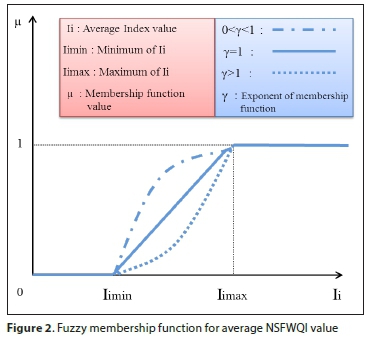
As noted before, the fuzzy set theory was used for the proposed model. Water quality standards according to PCA's goals were considered based on the average WQI value. The WQI which was applied here (i.e. NSFWQI) was a decreasing index (value decreased with increasing pollution). Also, the water quality standards are usually restricted by bounds (into an interval). Suppose these standards are a fuzzy set. Based on the definition, a membership function of each fuzzy set has to select a continuous and real value between 0 and 1. In accordance with the above-mentioned issues, the appropriate membership function (linear or nonlinear) for average WQI is given as follows:

where μ(Ii) is the membership function of fuzzy set, Ii is average NSFWQI for all checkpoints in the river system for ant i, Iimin and Iimax are the minimum and maximum of 7i, respectively, and y is the exponent of membership function and non-zero real number. This membership function is plotted in Fig. 2.
To calculate the optimum value of average NSFWQI in the river system, the following model was proposed:
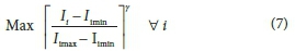
Subject to:
where Ijfis the average NSFWQI value for the ant i in the checkpoint j (the same NSFWQI value in Eq. 1), Iijminand Ijmax are the minimum and maximum values of Iij respectively, Ckis total wastewater treatment costs for all treatment units in the river system and scenario k, Cklis wastewater treatment cost for scenario k and treatment unit l, Ckminand Ckmaxare the minimum and maximum Cklvalues, respectively, NCP is the number of the checkpoints in the river system and ND is the number of treatment units. Other parameters were defined above.
Equation 7 is the objective function that was considered in the proposed model. Equations 8 and 9 are crisp constraints related to the PCA's goal and limit the average amount of NSFWQI and NSFWQI values in each river checkpoint, respectively. Equations 10 and 11 are crisp constraints related to the discharger's goal and limit the total wastewater treatment cost and the amount of treatment cost in each treatment unit, respectively. Equations 12 and 13 address the method of calculating the average amount of NSFWQI and the total treatment cost, respectively (Sasikumar and Mujumdar, 1998; Zimmermann, 2011; Cullis et al., 2018; De Ketele et al., 2018; Namugize and Jewitt, 2018).
Simulation-optimization (S-O) approach
The S-O approach is one of the most practical techniques for solving the quality and quantity problems that determine the required problem parameters with the use of a suitable simulation program or model in the first stage, and determines the optimum problem solutions extracted from the results of the simulation model with the use of a suitable optimization algorithm in the second stage (Saadatpour and Afshar, 2007; Skardi et al., 2015; Mooselu et al., 2019a; Dehghanipour et al. 2020).
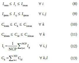
As stated in the previous sections, in this research the S-O approach was used to link the WLA model to a water quality simulation model. The simulator model used here was QUAL2K and the optimizer model was the ACO algorithm. The implementation stages of the S-O approach for solving the proposed model are presented in Fig. 3.
The following steps present a perfect description of this approach:
Step 1. Before starting, the initial data extracted from Mostafavi (2010) have been entered into the simulator model. Initial data include the hydraulic characteristics of the river, water quality characteristics (such as the concentration of the untreated WQPs in each of the treatment units), and constant coefficients and parameters in the equations imposed on the water quality problems. Then, the optimizer program is implemented.
Step 2. At first, the number of program iterations and the number of required ants for running the program are specified. To do this, an initial pheromone trail is done and the amount equal to each one for all the paths is defined. There are different criteria for specifying the number of appropriate iterations for the optimizer algorithm. One of the criteria is to increase the number of iterations until an appropriate convergence is achieved in the path of all ants.
Step 3. One ant selects various scenarios for each of the treatment units based on a relatively random process. Now, the simulator model is used.
Step 4. Based on the selective scenarios, different levels of pollutants are removed by the units which discharge into the river.
Step 5. The simulator model runs based on the initial data (in Step 1) and the fractional removal levels of pollutants (in Step 4) and then returns the amount of the WQPs in different parts of the river as output data. Furthermore, the optimizer model is run.
Step 6. The index value of each of the WQPs is calculated for all river checkpoints. The relationship between the amount or concentration of WQPs and their respective index values are presented by the special curves (such as the one shown in Fig. 1). In order to use these figures in the optimizer model, after fitting more than 100 effective points of the curves, the equations of the index value based on concentration value for all WQPs with high precision are extracted and the optimizer model is given.
Step 7. The index value is calculated (based on Eq. 1) for each of the river checkpoints. In this step, if the considered ant is not the final ant, there is a return to Step 3; otherwise, it is continued from Step 8. Also, if Constraints 9 and 11 are not established, the next iteration should be followed and Step 3 should be started.
Step 8. At first, the average values of NSFWQI are calculated for all ants (according to Eq. 12). Then, these values are replaced in the fuzzy membership function and their maximum values are selected. If Constraints 8 and 10 are not established, the program should go to the next iteration.
Step 9. In this step, updating of the pheromone concentration takes place based on the maximum value of the objective function (according to Eqs. 4 and 5). All of the above steps will be repeated to the final iteration which was considered for the optimizer program.
Case study
To evaluate the performance ofthe proposed model, a hypothetical river system (Mostafavi, 2010) with a length of 30 km was used (Fig. 4).

As can be seen in Fig. 4, the river included 6 river reaches and 5 dischargers that discharge wastewater into the river. Here, there were 16 separate elements and, in the midst of these elements, there were the considered checkpoints. The inlet and outlet of the river were considered as the checkpoints; therefore, there were 17 checkpoints in the river system. The river has a wide rectangular cross-section and the average air temperature in the location of the river was 20°C (Mostafavi, 2010).
To determine the re-aeration coefficient, the O'Conner and Dobbins equation was used (Sasikumar and Mujumdar, 1998). The hydraulic characteristics of the river are given in Table 1. The characteristics of the untreated wastewater for each of the treatment units as well as the river upstream are given in Table 2. The concentration of the total suspended solids (TSS) given in this table plays an important role in the calculations of the simulator model. However, it is ineffective in the determination of the WQI value. Fractional removal levels associated with different scenarios and wastewater treatment costs associated with the treatment units are given in Tables 3 and 4, respectively. The number of parameters intended for the proposed and the optimizer model can be seen in Table 5. NA in the table is the number of artificial ants applied to the optimizer model. The values in this table have been determined based on previous studies (Van Note et al., 1975; Sasikumar and Mujumdar, 1998; Eheart and Ng, 2004; Afshar et al., 2009; Mostafavi, 2010) and trial-and-error during the model execution.
RESULTS AND DISCUSSION
In this section, the results of the proposed model implementation are investigated and analysed. The model was executed on a hypothetical river (see Fig. 4) with the specifications and data given in Tables 1 to 5. This model was analysed by 30 successful and acceptable implementations of different values of q0and y.
As mentioned before, q0is the regulatory parameter of the ACO algorithm and y is the exponent of the membership function of average NSFWQI. At first, the obtained solution from the QUAL2K was examined with 100 and 150 iterations. As complete stability was not achieved in the solution (i.e., the ant path) in some cases, 200 iterations of parameters q0and y were used. As a result, the QUAL2K model was underwent 200 iterations for each optimal solution. Also, 20 artificial ants were preferred for searching the random paths in the optimizer algorithm. The objective function values obtained with 30 implementations of the optimizer program for each of the various values of q0(0.6, 0.7, 0.8, and 0.9) and y (0.5 and 2) are shown in Figs 5 and 6.


As can be seen, the objective function values was highest for q0= 0.6 and lowest for q0= 0.9. For q0= 0.6 and q0= 0.7 in different implementations of the optimizer program, these values were similar and, comparatively, identical. Based on these figures, reduction of q0from 0.9 to 0.6 led to a decrease in exploitation and increase in exploration in searching for the next path by ants. In other words, in this model, ants prefer to search more newly discovered paths and there is less likelihood of choosing the paths with a higher concentration of pheromone on which the best ants have passed. Based on these figures, it can be inferred that the objective function values obtained from the model equal to 0.6 and 0.7 were more appropriate, and the exploitation phenomenon was prominent in determining the optimum solutions. Statistical analysis of the data from Figs 5 and 6 and other outputs of the program is presented in Table 6.
In Columns 3 to 7, statistical elements of objective function values for 1 to 30 program implementation iterations are given. Columns 8 to 10 include the data associated with the maximum objective function values (based on data in Column 3). In Columns 11 to 15, the selective scenario number is given for the treatment units according to the maximum values of the objective function.
These data can help in understanding and analysing the model. A brief analysis of the data in the table is offered below:
1. The appropriate solutions in the proposed model can be the same as the maximum values of the objective function which are obtained for q0equal to 0.6 and 0.7. Also, in this case, and for each of the y values, the maximum values of the corresponding objective function had the same values. This is why the data of Columns 9 to 15 demonstrated the same values for values of q0 equal to 0.6 and 0.7. These q0 included the same values of the average index, the same total cost, and also the same treatment scenario number.
2. For q0 equal to 0.6 and y values equal to 0.5 and 1, the solutions were obtained by 30 runs of the optimizer program. Therefore, it is concluded that obtaining appropriate solutions is possible by implementing a few runs of the optimization model, and this can increase the chances of finding the solutions. Besides, the standard deviation values for y = 1 were less than that for y = 0.5. So, the case of q0 = 0.6 and y = 1 can be considered as the best possible solution; therefore, the more appropriate objective function of the model was equal to 0.1565 and the total wastewater treatment costs for all the treatment units was 3.98 million USD/yr and the optimal scenarios related to the units of 1 to 5 were 10, 10, 10, 10 and 11, respectively.
3. For q0equal to 0.6 and values of y equal to 0.5 and 1, the maximum value of the objective function was equal to the mode value, i.e., the maximum value of the objective function had the highest iteration obtained from running the optimizer program 30 times, while the maximum value of the objective function was repeated only once according to Column 8 in Table 6. On the other hand, for q0= 0.9 and y = 2, the minimum value of the objective function was equal to the mode value; generally, it can be observed that by increasing the value of q0from 0.6 to 0.9 the program deviates from the optimal solutions and searches the nonoptimal solutions. It is recommended that, for high values of q0, the number of program iterations is extremely high, although the maximum obtained values might not be very suitable.
4. As is evident from Points 1 and 2, the set of obtained solutions associated with q0 values equal to 0.6 and 0.7 can be considered as the optimal solutions of the model. Also, because of the negligible difference between the maximum and minimum values of the objective function for two of the q0, these show the lowest standard deviation among all q0 values studied. The same results can be observed for q0 = 0.9 and y = 2. The standard deviation values are shown in Column 6 of Table 6. This means that, under these conditions, less time and a lower number of the program's executions (less than 30 times) can lead to near-optimal solutions (not necessarily optimal).
5. According to the contents of Point 3 and the data presented in Table 6, it can be stated that for the values of q0equal to 0.6 and 0.7, the standard deviation of the data was lowest and the difference between the values of the model and maximum values of the objective function was less related to other conditions of the problem. Therefore, it can require less time and fewer program iterations (less than 30) to obtain optimal solutions. Also, for q0 values equal to 0.8 and 0.9, in which the standard deviation of the data was high and the difference between mode value and the maximum value of the objective function was higher than those for other q0values, the iteration number of the optimizer model for obtaining the optimal solutions becomes much higher. In this condition, the obtained maximum solutions were not optimal.
6. Figs 7 and 8 show the curves related to the NSFWQI values for 17 checkpoints of the river associated with the maximum values of the objective function for different values of q0 and for values of y equal to 0.5 and 2, respectively.


The values of the WQI index between Checkpoints 1 to 3 are the same in all cases because based on the hypothetical river structures (Fig. 4), the first wastewater treatment unit was located on the border of Checkpoints 1 to 3. So these checkpoints had the same qualitative behaviour. There are large jumps at Checkpoints 3, 6, 10, 12, and 14 which showed the establishment of 5 wastewater treatment units before the border checkpoints and drastically altered the behaviour of the river water quality parameters.
CONCLUSION
In this study, a WLA optimization model using the constraints of the wastewater treatment costs along with the objective function of the average NSFWQI and fuzzy approach was proposed. The use of the NSFWQI accelerates the understanding of the water quality in rivers and the fuzzy approach can decrease the uncertainties related to the model goals. Also, the S-O approach with the QUAL2K simulator model and the ACO algorithm were applied for solving the problem. The use of the S-O approach accelerates the program's execution. The model results showed that for the regulatory parameter of the ACO algorithm, i.e., q0, values equal to 0.6 or 0.7, and for the exponent of the membership function of the average NSFWQI, i.e., y values equal to 0.5, 1 and 2, the objective function has the maximum value and the results are the best possible values. In this case, treatment costs, average NSFWQI values, and appropriate scenarios for river system management will be obtained. This model is expansible; it can be developed for multi-objective models in the future, considering other uncertainties and constraints. Hence, planning and management of the water resources can be undertaken using a more complete and integrated approach.
REFERENCES
ABBASI T and ABBASI SA (2012) Water Quality Indices. Elsevier, Amsterdam. [ Links ]
AFSHAR A, MASSOUMI F, AFSHAR A and MARINO MA (2015) State of the art review of ant colony optimization applications in water resource management. Water Resour. Manage. 29 (11) 3891-3904. https://doi.org/10.1007/s11269-015-1016-9 [ Links ]
AFSHAR A, SHARIFI F and JALALI MR (2009) Non-dominated archiving multi-colony ant algorithm for multi-objective optimization: Application to multi-purpose reservoir operation. Eng. Optim. 41 (4) 313-325. https://doi.org/10.1080/03052150802460414 [ Links ]
ASHTIANI EF, NIKSOKHAN MH and JAMSHIDI S (2015) Equitable fund allocation, an economical approach for sustainable waste load allocation. Environ. Monit. Assess. 187 (8) 522. https://doi.org/10.1007/s10661-015-4739-4 [ Links ]
AZAD A, FARZIN S, KASHI H, SANIKHANI H, KARAMI H and KISI O (2018a) Prediction of river flow using hybrid neuro-fuzzy models. Arab. J. Geosci. 11 (22) 718. https://doi.org/10.1007/s12517-018-4079-0 [ Links ]
AZAD A, KARAMI H, FARZIN S, SAEEDIAN A, KASHI H and SAYYAHI F (2018b) Prediction of water quality parameters using ANFIS optimized by intelligence algorithms (case study: Gorganrood River). KSCE J. Civ. Eng. 22 (7) 2206-2213. https://doi.org/10.1007/s12205-017-1703-6 [ Links ]
BABAEE TIRKOLAEE E, MAHDAVI I, SEYYED ESFAHANI MM and WEBER GW (2020) A hybrid augmented ant colony optimization for the multi-trip capacitated arc routing problem under fuzzy demands for urban solid waste management. Waste Manage. Res. 38 (2) 156-172. https://doi.org/10.1177/0734242X19865782 [ Links ]
BROWN RM, MCCLELLAND NI, DEININGER RA and TOZER RG (1970) A water quality Index - do we dare? Water Sewage Works. 117 (10) 339-343. [ Links ]
CULLIS JD, ROSSOUW N, DU TOIT G, PETRIE D, WOLFAARDT G, CLERCQ WD and HORN A (2018) Economic risks due to declining water quality in the Breede River catchment. Water SA. 44 (3) 464473. https://doi.org/10.4314/wsa.v44i3.14 [ Links ]
DE KETELE J, DAVISTER D and IKUMI DS (2018) Applying performance indices in plantwide modelling for a comparative study of wastewater treatment plant operational strategies. Water SA. 44 (4) 539-350. https://doi.org/10.4314/wsa.v44i4.03 [ Links ]
DEHGHANIPOUR AH, SCHOUPS G, ZAHABIYOUN B and BABAZADEH H (2020) Meeting agricultural and environmental water demand in endorheic irrigated river basins: A simulation-optimization approach applied to the Urmia Lake basin in Iran. Agric. Water Manage. 241 106353. https://doi.org/10.1016/j.agwat.2020.106353 [ Links ]
DORIGO M and GAMBARDELLA LM (1997) Ant colony system: a cooperative learning approach to the traveling salesman problem. IEEE Trans. Evol. Comput. 1 (1) 53-66. https://doi.org/10.1109/4235.585892 [ Links ]
DORIGO M and STUTZLE T (2019) Ant colony optimization: overview and recent advances. In: Handbook of Metaheuristics. Springer, Cham. 311-351. https://doi.org/10.1007/978-3-319-91086-4_10 [ Links ]
EHEART JW and NG TL (2004) Role of effluent permit trading in total maximum daily load programs: overview and uncertainty and reliability implications. J. Environ. Eng. 130 (6) 615-621. https://doi.org/10.1061/(ASCE)0733-9372(2004)130:6(615) [ Links ]
ESTALAKI SM, ABED-ELMDOUST A and KERACHIAN R (2015) Developing environmental penalty functions for river water quality management: application of evolutionary game theory. Environ. Earth Sci. 73 (8) 4201-4213. https://doi.org/10.1007/s12665-014-3706-7 [ Links ]
FARZADKHOO M, KESHAVARZI A, HAMIDIFAR H and JAVAN M (2018) A comparative study of longitudinal dispersion models in rigid vegetated compound meandering channels. J. Environ. Manage. 217 78-89. https://doi.org/10.1016/j.jenvman.2018.03.084 [ Links ]
FARZADKHOO M, KESHAVARZI A, HAMIDIFAR H and JAVAN M (2019) Sudden pollutant discharge in vegetated compound meandering rivers. Catena. 182 104155. https://doi.org/10.1016/j.catena.2019.104155 [ Links ]
FENG Y, BAO Q, CHENGLIN L, BOWEN W and ZHANG Y (2018) Introducing biological indicators into CCME WQI using variable fuzzy set method. Water Resour. Manage. 32 (8) 2901-2915. https://doi.org/10.1007/s11269-018-1965-x [ Links ]
GHOLIZADEH H and FAZLOLLAHTABAR H (2020) Robust optimization and modified genetic algorithm for a closed loop green supply chain under uncertainty: Case study in melting industry. Comput. Ind. Eng. 147 106653. https://doi.org/10.1016/j.cie.2020.106653 [ Links ]
HAMIDIFAR H, OMID MH and KESHAVARZI A (2015) Longitudinal dispersion in waterways with vegetated floodplain. Ecol. Eng. 84 398-407. https://doi.org/10.1016/j.ecoleng.2015.09.048 [ Links ]
HASANZADEH SK, SAADATPOUR M and AFSHAR A (2020) A fuzzy equilibrium strategy for sustainable water quality management in river-reservoir system. J. Hydrol. 124892. https://doi.org/10.1016/j.jhydrol.2020.124892 [ Links ]
HUANG S, CHANG J, LENG G and HUANG Q (2015) Integrated index for drought assessment based on variable fuzzy set theory: a case study in the Yellow River basin, China. J. Hydrol. 527 608-618. https://doi.org/10.1016/j.jhydrol.2015.05.032 [ Links ]
KALHOR E, KHANZADI M, ESHTEHARDIAN E and AFSHAR A (2011) Stochastic time-cost optimization using non-dominated archiving ant colony approach. Autom. Constr. 20 (8) 1193-1203. https://doi.org/10.1016/j.autcon.2011.05.003 [ Links ]
KANNEL PR, LEE S, LEE YS, KANEL SR and KHAN SP (2007) Application of water quality indices and dissolved oxygen as indicators for river water classification and urban impact assessment. Environ. Monit. Assess. 132 (1-3) 93-110. https://doi.org/10.1007/s10661-006-9505-1 [ Links ]
KARMAKAR S and MUJUMDAR PP (2006) Grey fuzzy optimization model for water quality management of a river system. Adv. Water Resour. 29 (7) 1088-1105. https://doi.org/10.1016/j.advwatres.2006.04.003 [ Links ]
LEI K, ZHOU G, GUO F, KHU ST, MAO G, PENG J and LIU Q (2015) Simulation-optimization method based on rationality evaluation for waste load allocation in Daliao river. Environ. Earth Sci. 73 (9) 5193-5209. https://doi.org/10.1007/s12665-015-4334-6 [ Links ]
LIU Y, WANG C, CHUN Y, YANG L, CHEN W and DING J (2019) A novel method in surface water quality assessment based on improved variable fuzzy set pair analysis. Int. J. Environ. Res. Public Health. 16 (22) 4314. https://doi.org/10.3390/ijerph16224314 [ Links ]
MAHJOURI N and ABBASI MR (2015) Waste load allocation in rivers under uncertainty: application of social choice procedures. Environ. Monit. Assess. 187 (2) 5. https://doi.org/10.1007/s10661-014-4194-7 [ Links ]
MARKS SJ, KUMPEL E, GUO J, BARTRAM J and DAVIS J (2018) Pathways to sustainability: A fuzzy-set qualitative comparative analysis of rural water supply programs. J. Cleaner Prod. 205 789798. https://doi.org/10.1016/j.jclepro.2018.09.029 [ Links ]
MELLAL MA and WILLIAMS EJ (2018) A survey on ant colony optimization, particle swarm optimization, and cuckoo algorithms. In: Vasant P, Alparslan-Gok SZ and Weber GW (eds) (2017) Handbook of Research on Emergent Applications of Optimization Algorithms. IGI Global, . 37-51. https://doi.org/10.4018/978-1-5225-2990-3.ch002 [ Links ]
MOOSELU MG, NIKOO MR, RAYANI NB and IZADY A (2019a) Fuzzy multi-objective simulation-optimization of stepped spillways considering flood uncertainty. Water Resour. Manage. 33 (7) 22612275. https://doi.org/10.1007/s11269-019-02263-2 [ Links ]
MOOSELU MG, NIKOO MR and SADEGH M (2019b) A fuzzy multi-stakeholder socio-optimal model for water and waste load allocation. Environ. Monit. Assess. 191 (6) 359. https://doi.org/10.1007/s10661-019-7504-2 [ Links ]
MOSTAFAVI SA (2010) Waste load allocation in river systems with multi-objective approach. MSc thesis, School of Civil Engineering, Iran University of Science and Technology (in Persian). [ Links ]
NADA A, ELSHEMY M, ZEIDAN BA and HASSAN AA (2016) Water quality assessment of Rosetta Branch, Nile River, Egypt. In: Third International Environmental Forum, Environmental Pollution: Problem and Solution, 12-14 July, Tanta University, Egypt. [ Links ]
NAMUGIZE JN and JEWITT GP (2018) Sensitivity analysis for water quality monitoring frequency in the application of a water quality index for the uMngeni River and its tributaries, KwaZulu-Natal, South Africa. Water SA. 44 (4) 516-527. https://doi.org/10.4314/wsa.v44i4.01 [ Links ]
NAYAK J, VAKULA K, DINESH P, NAIK B and MISHRA M (2020) Ant colony optimization in data mining: critical perspective from 2015 to 2020. In: Innovation in Electrical Power Engineering, Communication, and Computing Technology. Springer, Singapore. 361-374. https://doi.org/10.1007/978-981-15-2305-2_29 [ Links ]
NIKOO MR, BEIGLOU PH and MAHJOURI N (2016) Optimizing multiple-pollutant waste load allocation in rivers: an interval parameter game theoretic model. Water Resour. Manage. 30 (12) 4201-4220. https://doi.org/10.1007/s11269-016-1415-6 [ Links ]
QIN X, HUANG G, CHEN B and ZHANG B (2009) An interval-parameter waste-load-allocation model for river water quality management under uncertainty. Environ Manage. 43 (6) 999-1012. https://doi.org/10.1007/s00267-009-9278-8 [ Links ]
SAADATPOUR M and AFSHAR A (2007) Waste load allocation modeling with fuzzy goals; simulation-optimization approach. Water Resour. Manage. 21 (7) 1207-1224. https://doi.org/10.1007/s11269-006-9077-4 [ Links ]
SABERI L and NIKSOKHAN MH (2017) Optimal waste load allocation using graph model for conflict resolution. Water Sci. Technol. 75 (6) 1512-22. https://doi.org/10.2166/wst.2016.429 [ Links ]
SASIKUMAR K and MUJUMDAR PP (1998) Fuzzy optimization model for water quality management of a river system. J. Water Resour. Plann. Manage. 124 (2) 79-88. https://doi.org/10.1061/(ASCE)0733-9496(1998)124:2(79) [ Links ]
SKARDI MJE, AFSHAR A, SAADATPOUR M and SOLIS SS (2015) Hybrid ACO-ANN-based multi-objective simulation-optimization model for pollutant load control at basin scale. Environ. Model. Assess. 20 (1) 29-39. https://doi.org/10.1007/s10666-014-9413-7 [ Links ]
TAKYI AK and LENCE BJ (1996) Chebyshev model for water-quality management. J. Water Resour. Plann. Manage. 122 (1) 40-48. https://doi.org/10.1061/(ASCE)0733-9496(1996)122:1(40) [ Links ]
TAVAKOLI A, NIKOO MR, KERACHIAN R and SOLTANI M (2015) River water quality management considering agricultural return flows: application of a nonlinear two-stage stochastic fuzzy programming. Environ. Monit. Assess. 187 (4) 158. https://doi.org/10.1007/s10661-015-4263-6 [ Links ]
TEIXEIRA Z, DE OLIVEIRA VITAL SR, VENDEL AL, DE MENDONCA JDL and PATRICIO J (2020) Introducing fuzzy set theory to evaluate risk of misclassification of land cover maps to land mapping applications: Testing on coastal watersheds. Ocean Coast. Manage. 184 104903. https://doi.org/10.1016/j.ocecoaman.2019.104903 [ Links ]
TYAGI S, SHARMA B, SINGH P and DOBHAL R (2013) Water quality assessment in terms of water quality index. Am. J. Water Resour. 1 (3) 34-38. https://doi.org/10.12691/ajwr-1-3-3 [ Links ]
VAN NOTE RH, HEBERT PV, PATEL RM, CHUPEK C and FELDMAN L (1975) A guide to the selection of cost-effective wastewater treatment systems, Technical Report prepared for Office of Water Program Operations, United States Environmental Protection Agency. USEPA, Washington, D.C. [ Links ]
WONG BK and LAI VS (2011) A survey of the application of fuzzy set theory in production and operations management: 19982009. Int. J. Prod. Econ. 129 (1) 157-168. https://doi.org/10.1016/j.ijpe.2010.09.013 [ Links ]
XU J, HOU S, YAO L and LI C (2017) Integrated waste load allocation for river water pollution control under uncertainty: a case study of Tuojiang River, China. Environ. Sci. Pollut. Res. 24 (21) 17741-17759. https://doi.org/10.1007/s11356-017-9275-z [ Links ]
ZIMMERMANN HJ (2011) Fuzzy Set Theory-and its Applications. Springer Science & Business Media, Dordrecht, Netherlands. [ Links ]
 Correspondence:
Hossein Hamidifar
Email: hamidifar@shirazu.ac.ir
Received: 3 September 2019
Accepted: 18 December 2020

