RESEARCH PAPER

 

Modelling groundwater level fluctuation in an Indian coastal aquifer

 

 

Safieh Javadinejad; Rebwar Dara; Forough Jafary

Department of Geography, Environment and Earth sciences University of Birmingham, Edgbaston St., B152TT, United Kingdom

Correspondence

 

 

---

ABSTRACT

Estimating groundwater level (GWL) fluctuations is a vital requirement in hydrology and hydraulic engineering, and is commonly addressed through artificial intelligence (AI) models. The purpose of this research was to estimate groundwater levels using new modelling methods. The implementation of two separate soft computing techniques, a multilayer perceptron neural network (MLPNN) and an M5 model tree (M5-MT), was examined. The models are used in the estimation of monthly GWLs observed in a shallow unconfined coastal aquifer. Data for the water level were collected from observation wells located near Ganjimatta, India, and used to estimate GWL fluctuation. To do this, two scenarios were provided to achieve optimal input variables for modelling the GWL at the present time. The input parameters applied for developing the proposed models were a monthly time-series of summed rainfall, the mean temperature (within its lag times that have an effect on groundwater), and historical GWL observations throughout the period 1996-2006. The efficiency of each proposed model for Ganjimatt was investigated in stages of trial and error. A performance evaluation showed that the M5-MT outperformed the MLPNN model in estimating the GWL in the aquifer case study. Based on the M5-MT approach, the development of this model gives acceptable results for the Indian coastal aquifers. It is recommended that water managers and decision makers apply these new methods to monitor groundwater conditions and inform future planning.

Keywords: groundwater level estimation, multilayer perceptron, neural network,, M5 model tree, Indian coastal aquifers, time-series modelling

---

 

 

INTRODUCTION

Analysis of groundwater levels (GWL) within hydrological and hydraulic studies, particularly in developing countries where overexploitation is a problem, is crucial. This will also lead to effective and integrated management and planning for groundwater resources in the future (Javadinejad et al., 2019a).

Accurate assessments of groundwater levels allow water directors, engineers, and stakeholders to improve policies designed to prevent or decrease detrimental impacts, e.g., a pumping deficit in water wells, land surface collapse, aquifer compression, and poor water quality (Prinos et al., 2002). Furthermore, these evaluations, along with predictive modelling, are beneficial in developing a better understanding of the dynamics and underlying factors that affect groundwater (Javadinejad et al., 2019b). This understanding can help to balance the needs of urban, agricultural, and industrial water uses, and to trade off profits and prices of water protection (Adamowski and Fung Chan, 2011; Moosavi et al., 2013).

While theoretical and physically based models are significant tools to define the physical progressions and variables of hydrology, they have practical restrictions and limitations (Nourani et al., 2008, 2011). Calibrations of these models are very difficult, since many parameters need to be controlled, particularly in chalky media. Additionally, these models need an enormous quantity of good data and a complete realisation of the essential physical processes in the system (Chen et al., 2009). Sometimes data are not adequate, and more precise forecasts are easier to achieve than real data. In this case, empirical models may be suitable substitute techniques, where some data are accessible over an extended period of time.

In the current decade, soft computing methods, including artificial neural networks (ANN), gene expression programming (GEP), group methods of data handling (GMDH), adaptive neuro-fuzzy interference systems (ANFIS), and support vector machine (SVM) techniques, have been utilized as suitable approaches to estimate complex non-linear time-series in hydrological processes and hydraulic engineering (Shiri and Kisi, 2011; Etemad-Shahidi and Taghipour, 2012; Kisi et al., 2013; Najafzadeh and Zahiri, 2015; Hosseini and Mahjouri, 2016; Kisi and Parmar, 2016; Najafzadeh et al., 2016; Rahimikhoob, 2016; Zeroual et al., 2016). Among these soft computing techniques, ANNs provide an interesting means to model systems of water supplies (Maier and Dandy, 2000). Multilayer perceptron (MLP) feed-forward network types have been extensively used to model hydrological processes (Isik et al., 2013). Additionally, soft computing methods have been used for assessment of GWL fluctuations. For example, Shiri and Kisi (2011) evaluated the implementation of genetic programming (GP) and an adaptive neuro-fuzzy inference system (ANFIS) to predict groundwater level fluctuations using several benchmarks. According to their findings, the performance of GP was relatively better than that of the ANFIS model.

A second example is the work of Shiri et al. (2013), who investigated the performance of adaptive ANFIS, support vector regression (SVM), GEP, and also ANN models to estimate the depth of GW. They concluded that GEP provided the most precise prediction compared with other models.

Another example is Mohanty et al. (2015), who made use of ANN in order to forecast the levels of GW in multiple wells within a river basin. Their results showed that the ANN model was a useful method for GWL prediction. The model performed better and even outperformed in a shorter period of time those which ran over a longer period. Many AI approaches based on data-driven models, such as a multilayer perceptron neural network (MLPNN) and the M5 model tree (M5-MT), can obtain a robust correlation between predicted and observed values to estimate monthly GWL fluctuations.

Successful applications of black-box models in water resource considerations have inspired the exploration of their ability to estimate GWL fluctuations. Extending the previous studies reviewed in the introduction, the focus of this research was to examine the capability of the MLPNN and M5-MT to estimate monthly GWL fluctuations. The previous studies did not analyse and compare the MLPNN and M5-MT results, and did not monitor the groundwater level fluctuations. So, the purpose of this study was to estimate groundwater-level fluctuations using the new models, MLPNN and M5-MT. This paper presents some important points regarding the MLPNN and M5-MT; it documents the development of the proposed models for GWL estimation; and it describes this further using a case study.

 

METHODOLOGY

Forecasting hydrological processes is one of the important elements in providing reliable and accurate applications for water resource management. The M5 MT has rarely been used for hydrological issues (e.g. rainfall-runoff modelling, flood forecasting, groundwater modelling). It should be noted that one of the key aspects in using M5 MT is its capability to provide mathematical functions that show the relationship between the variables of input-output; which is not the case for the MLPNN model. The development of the two different soft computing techniques, the traditional MLPNN and M5 MT approaches, applied to estimate monthly GWL fluctuations, is briefly described in this section.

Multilayer perceptron neural network (MLPNN)

The ANN computational method is inspired by the biological nervous system which is the basis of the human brain. The most noteworthy benefit of this method compared to conventional hydrological models is its ability to successfully identify both the linear and non-linear hydrologic relationships between the inputs and outputs. Furthermore, the ANN model can adapt itself to altering conditions which lead to model implementation improvement; it reduces computation time and accelerates simulation enhancement (Cigizoglu et al., 2004). Though there are various kinds of ANN, the multilayer perceptron neural network (MLPNN) is the most widely used in resolving hydrological problems (McGarry et al., 1999). The network of the MLPNN can be comprised of one or many neurons and layers, but generally contains three layers: (i) the input layer, through data entering the network; (ii) the unseen layer or layers, where data are processed; and (iii) the output layer, which is responsible for producing a suitable reaction to the particular inputs.

To construct a neural network, the number of layers, the number of neurons in each layer, and the incitement occupation of each neuron, should be determined to minimize errors. Various methods are available to minimize errors, such as the Levenberg-Marquardt algorithm, steepest descent, conjugating the gradient algorithm, the Bayesian approach, and the momentum approach. These methods can also increase the speed of analysis, and follow a back-propagation approach. Firstly, some random principles are appointed to the weight and bias of each neuron. Subsequently, the preliminary testing sample vector is fed into the network and the output computed and contrasted to the available observed data. This process is followed by modifying weights or parameters using an iterative algorithm in order to reduce the error size (Abbasifarfani et al., 2015). More information on ANN structures can be found in Haykin (2004).

M5 model tree (M5-MT)

The M5 model tree is a supervised learning technique which has been widely used in numeric modelling. This method was first presented by Quinlan (1992), and then Wang and Witten (1997) improved the technique in an algorithm named M5 (Esmaeilzadeh et al., 2017). The model tree is a tree that contains a root node and leaves with functions of linear regression at the top and bottom of the tree. The main purpose of this model is to determine the relevance of independent and dependent variables (Witten and Frank, 2005). The distribution interval of input variables can help to create a better linear regression and is one of the benefits of a model tree that can increase the model's precision. (Najafzadeh et al., 2016).

The algorithm follows two separate steps: (i) the development of the tree; and (ii) the tree pruning. Firstly, the M5 algorithm builds a tree of regression through repeated splitting of the example interval. The splitting circumstance can decrease the intra-subset changeability in the principles down from the root, over the division to the node. The changeability is assessed through the standard deviation of the principles that lead from the root to the node via the branch. The projected decrease in error is computed due to the examination of each element at the node. Afterwards, the element which causes the projected error to decrease is selected. If the elements of all output examples that receive a node change marginally, or just a small number of data records remain, then the splitting progression ceases (Witten and Frank, 2005).

To organize the basic tree, standard deviation reduction (SDR) is applied as a splitting criterion in the M5 model tree. This criterion is computed as:

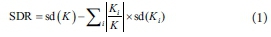
where K indicates a series of data that receive the node; K represents the subdivisions of data that have the i^th result of the possible set; and sd is the standard deviation (Witten and Frank, 2005). The splitting progression drives the child node to have minor principles of standard deviation, in contrast to the parent node; therefore, they are purer (Quinlan, 1992). After assessing all the probable splits, the design of the M5 model tree selects the split that increases the projected error decrease. This data dissection created throughout the M5 algorithm process creates a large tree, which can be the reason for the over-matching with the examined data. To solve the problem of over-fitting, Quinlan (1992) proposed applying some reducing methods to cut back the too widely spread branches. Generally, pruning is done through substituting a subtree with a linear regression occupation. More information in this regard can be found in Quinlan (1992) and Witten and Frank (1997).

Description of the study region and data analysis

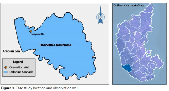
In this research, the selected well for the development of the proposed model is located in a neighbouring micro-watershed, under the Gurpura river basin. The well in Ganjimatta is located at 12°59'02" N and 74°57'15" E (Fig. 1). The study region is affected by the southwest monsoon (June-September) and a non-monsoon episode (October-May). The mean annual rainfall across the basin is approximately 3 500 mm.

 

 

The principal soil in this investigation is lateritic, which is extremely porous and permeable in nature. Because of its characteristics, the rate of penetration is maximum and any shallow wells react quickly to rainfall; thus increase the water table. However, its reaction to a decreasing trend is also fast.

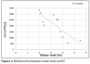
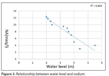
The quality of groundwater in this area depends on the amount of time between it being concentrated in the atmosphere and being discharged through a well. Any decrease in the water level leads to an increase in groundwater salinity. Groundwater salinity levels vary with respect to the aquifer recharge quantity, together with the depth of the freshwater layer and the level of pollution. Figures 2 and 3 show a relationship between the water level and quality (indicated by electrical conductivity and sodium) for 1996-2006. From 1996 to 2006, water quality has decreased. Also, the value for R² (>0.5) shows a strong relationship between the water level and water quality.

 

 

 

 

The main input to the groundwater level in the small catchment is from the monsoon rainfall data. The rainfall data that was estimated for the rain gauge stations and used in this study came from the National Institute of Technology Karnataka (NITK) campus. The rainfall data from this station for 1996-2006 was applied in this research. The average temperature and monthly rainfall data points within their lag times, and previous groundwater level observations, were applied in order to associate these with the magnitude of the groundwater level in the observation wells, on a monthly scale. The data were divided into two phases: approximately 70% (84 data points) of the dataset was applied for the training phase; whereas the remaining dataset (30%, 41 data points) was used for testing of the objectives.

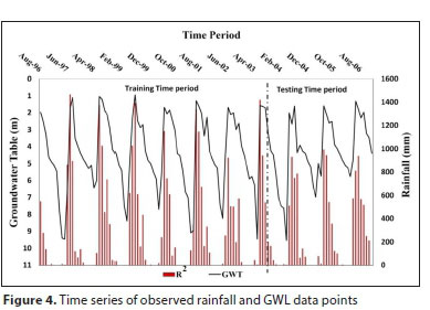
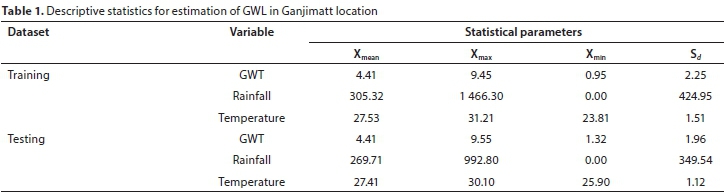
The water-table data for the observational well at Ganjimatta used in this study, between 1996 and 2006, was obtained from the Department of Mines and Geology, Dakshina Kannada District. From the data analysis, the maximum, minimum, mean, and standard deviation for all the variables that affect the GWL fluctuation for each of the training and testing phases are shown in Table 1. The time series of the observed rainfall and GWL fluctuations for the 1996-2006 period are indicated in Fig. 4.

 

 

Functional assessment criteria

In order to compare the rainfall-runoff simulation performance of the advanced models, various statistical indices (Eqs 2-4) were applied. The indices included correlation coefficient (R), root mean square error (RMSE) and relative absolute error (RAE):

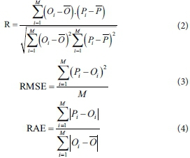
where O and P signify the observed run-off and projected run-off through the model, correspondingly; P is the average observed value; O indicates the average predicted value; and M indicates the whole number of dataset examples. R calculates how well the deliberated independent variables are credited for the calculated dependent variable. The RMSE is applied in order to calculate the estimated accuracy. The RMSE increases from zero as the precision of the evaluations increases, to large positive values, as the difference between modelled and observed values grow. The minor value of the RMSE and the major value of R (up to 1) indicate the high proficiency of the model. The RAE is the ratio of the absolute error in the measurement to the accepted measurement; a lower value of the RAE illustrates a good performance of the proposed model (Kisi and Parmar 2016; Rezaie-Balf and Kisi, 2017).

 

RESULTS AND DISCUSSION

Development of GWL simulation approaches

In this study, the MLPNN and M5-MT approaches were investigated to present monthly GWL forecasting at Ganjimatta. As there is no defined procedure for selecting the relevant inputs to forecast monthly GWL, two scenarios were applied using the MLPNN in the case study. These two scenarios (S1 and S2) are given below:

where GWL_(t-1), T_(t-1), and R_(t-1) represent previously recorded monthly groundwater levels, temperature, and rainfall values, respectively; the output corresponds to the GWL value at the current time (t).

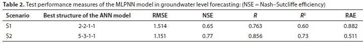
Thereafter, with calculating the statistical measures presented in Table 2, the optimal input combination was selected for forecasting the monthly GWL fluctuations in Ganjimatta.

The assessment of the MLPNN technique via the R, RMSE, and RAE is shown in Table 2. Two different MLPNN models with different configurations were applied for this location. The best structure of the ANN model, shown by '5-3-1-1' in the 2^nd column of Table 2, which represents an ANN model having 5 inputs, 3 non-linear hidden, 1 linear unseen, and 1 output node.

It is noteworthy that the optimal amount of neurons in the unseen layers, calculated via trial and error, began at 2 neurons. The number of neurons in each layer rose to 10 with a step size of 1.

Based on the performance evaluation (Table 2), it is clear that S2 (Scenario 2) for Ganjimatta has the higher correlation (R = 0.856), and the lower errors in terms of RMSE (1.151), and RAE (0.511) compared to S1 (R = 0.763, RMSE = 1.514 and RAE = 0.882).

The M5-MT procedure for estimation of GWL was applied by using open-source machine learning, Weka 3.6 software. The capability of M5-MT was evaluated in order to find the mathematical formulation in the form of linear relationships for GWL fluctuations' forecasting. The delinquency elements of the M5-MT method are designed for their delinquency values, a pruning factor of 4.0, and smoothing preference. After classifying, the model tree included 5 input and 1 output parameter, which was implemented to forecast the monthly GWL using several linear rules. These rules are based on conditional relationships presented as follows:

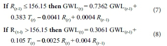
From these rules, it is clear that all input parameters except T_(t-1) were taken into account in the estimation of GWL, and were also significant in the development of the proposed linear models.

Comparison of the proposed models

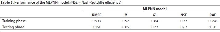
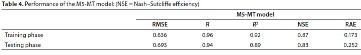
Two different artificial intelligence techniques were developed to forecast the monthly GWL fluctuations in Ganjimatta's observational well, which falls within the Gurpura River catchment. The performance of the tested approaches, analysed by computing the statistical error functions for monthly GWLs, is presented in Tables 3 and 4.

From the training phases, it can be seen that the M5-MT estimated the GWL with a higher correlation (R = 0.96) and lower statistical error (RMSE = 0.636) and RAE (0.173) compared to the MLPNN (R = 92, RMSE = 0.933 and RAE = 0.298). It should be noted that one of the key aspects of using M5-MT is the capability of this method to show the mathematical difference between the input and output variables, which is not the case in the MLPNN model.

From the results for the testing phase given in Tables 3 and 4, it can be noted that the proposed equation given by M5-MT estimated the monthly GWL with a higher accuracy than the MLPNN technique, similarly to the training phase.

Figures 5 and 6 show the proposed models' forecasts and detected GWL values for the training and testing phases, respectively. Also, the RMSE values (>0.05) indicate a good performance of the models.

 

 

 

 

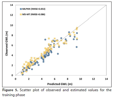
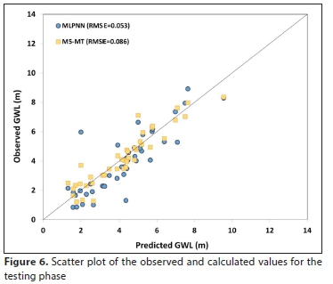
It can be shown that M5-MT predicts the groundwater level data more precisely than the MLPNN model; the projections of the M5-MT model are less dispersed and nearer to the trend-line than those of the MLPNN.

Figure 7 also illustrates the time-series of the observed versus calculated monthly GWL fluctuation, using the MLPNN technique in the training and testing phases. The figure indicates that the model is less precise for the large values than for the mid-values.

 

 

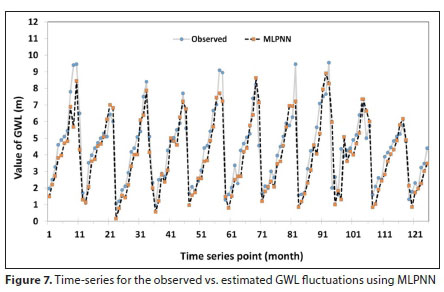
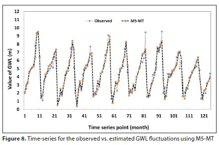
Figure 8 illustrates the time-series graphs of the predicted and observed monthly GWL forecasts in the training and testing phases, for the Ganjimatta case study with M5-MT. In contrast to MLPNN, M5-MT performed better in forecasting extreme values of GWL fluctuations. Also, RMSE values (>0.05) indicate a good performance of the model.

 

 

CONCLUSION

In this study, the MLPNN and M5-MT models were employed to model monthly groundwater level fluctuations using input from present and previous GWLs, temperatures, and rainfall from an observational well, located in Ganjimatta, Dankshina Kannada region of India.

The MLPNN model was tested by being applied to various input mixtures of the monthly groundwater levels, temperatures, and rainfall data points. After applying the MLPNN to select the optimal combination of inputs, the performances of the two proposed methods were evaluated based on R, RMSE, and RAE. The outcomes obtained indicated that the M5-MT model performed better than the MLPNN model in forecasting monthly GWLs for the studied well. The MLPNN model could not simulate the monthly GWL values for the observational well and the accuracy of this predictive model was generally found to be low. On the other hand, the M5-MT approach provided a better forecast for the extreme values than the MLPNN technique. The main advantage of the M5-MT model is its explicit mathematical formulations. It is simple to use in practical applications. By contrast, the MLPNN is a black-box model with concealed formulations. The proposed techniques may also be used in other hydrological applications (e.g. short-term wind speed predictions, seawater level forecasting, and prediction of daily evapotranspiration).

As an expansion to the present work, various data-derived methods such as GMDH and GEP can be applied and contrasted for GWL modelling in future studies.

 

REFERENCES

ADAMOWSKI J and CHAN HF (2011) A wavelet neural network conjunction model for groundwater level forecasting. J. Hydrol. 407 (1-4) 28-40. https://doi.org/10.1016/j.jhydrol.2011.06.013        [ Links ]

CIGIZOGLU HK (2004) Discussion of "Performance of Neural Networks in Daily Streamflow Forecasting" by S. Birikundavyi, R. Labib, HT Trung, and J. Rousselle. J. Hydrol. Eng. 9 (6) 556-557. https://doi.org/10.1061/(ASCE)1084-0699(2004)9:6(556)        [ Links ]

CHEN LH, CHEN CT and PAN YG (2009) Groundwater level prediction using SOM-RBFN multisite model. J. Hydrol. Eng. 15 (8) 624-631. https://doi.org/10.1061/(ASCE)HE.1943-5584.0000218        [ Links ]

ESMAEILZADEH B, SATTARI MT and SAMADIANFARD S (2017) Performance evaluation of ANNs and an M5 model tree in Sattarkhan Reservoir inflow prediction. ISH J. Hydraul. Eng. 23 (3) 283-292. https://doi.org/10.1080/09715010.2017.1308277        [ Links ]

ETEMAD-SHAHIDI A and TAGHIPOUR M (2012) Predicting longitudinal dispersion coefficient in natural streams using M5' model tree. J. Hydraul. Eng. 138 (6) 542-554. https://doi.org/10.1061/(ASCE)HY.1943-7900.0000550        [ Links ]

FARFANI HA, BEHNAMFAR F and FATHOLLAHI A (2015) Dynamic analysis of soil-structure interaction using the neural networks and the support vector machines. Expert Syst. Appl. 42 (22) 8971-8981. https://doi.org/10.1016Zj.eswa.2015.07.053        [ Links ]

HAYKIN S and NETWORK N (2004) A comprehensive foundation. Neural Networks. 2 (2004). 41. https://dl.acm.org/doi/book/10.5555/541500        [ Links ]

HOSSEINI SM and MAHJOURI N (2016) Integrating support vector regression and a geomorphologic artificial neural network for daily rainfall-runoff modeling. Appl. Soft Comput. 38 329-345. https://doi.org/10.1016/j.asoc.2015.09.049        [ Links ]

ISIK S, KALIN L, SCHOONOVER JE, SRIVASTAVA P and LOCKABY BG (2013) Modeling effects of changing land use/cover on daily streamflow: An artificial neural network and curve number based hybrid approach. J. Hydrol. 485 103-112. https://doi.org/10.1016/j.jhydrol.2012.08.032        [ Links ]

JAVADINEJAD S, HANNAH D, OSTAD-ALI-ASKARI K, KRAUSE S, ZALEWSKI M and BOOGAARD F (2019a) The impact of future climate change and human activities on hydro-climatological drought, analysis and projections: using CMIP5 climate model simulations. Water Conserv. Sci. Eng. 4 (2-3) 71-88. https://doi.org/10.1007/s41101-019-00069-2        [ Links ]

JAVADINEJAD S, OSTAD-ALI-ASKARI K and ESLAMIAN S (2019b) Application of multi-index decision analysis to management scenarios considering climate change prediction in the Zayandeh Rud River Basin. Water Conserv. Sci. Eng. 4 (1) 53-70. https://doi.org/10.1007/s41101-019-00068-3        [ Links ]

KISI O and PARMAR KS (2016) Application of least square support vector machine and multivariate adaptive regression spline models in long term prediction of river water pollution. J. Hydrol. 534 104-112. https://doi.org/10.1016/j.jhydrol.2015.12.014        [ Links ]

MAIER HR and DANDY GC (2000) Neural networks for the prediction and forecasting of water resources variables: a review of modelling issues and applications. Environ. Model. Software. 15 (1) 101-124. https://doi.org/10.1016/S1364-8152(99)00007-9        [ Links ]

MCGARRY KJ, WERMTER S and MACINTYRE J (1999) Knowledge extraction from radial basis function networks and multilayer perceptrons. In Proc. International Joint Conference on Neural Networks. 4 (5) 2494-2497. https://doi.org/10.1109/IJCNN.1999.833464        [ Links ]

MOHANTY S, JHA MK, RAUL SK, PANDA RK and SUDHEER KP (2015) Using artificial neural network approach for simultaneous forecasting of weekly groundwater levels at multiple sites. Water Resour. Manage. 29 (15) 5521-5532. https://doi.org/10.1007/s11269-015-1132-6        [ Links ]

MOOSAVI V, VAFAKHAH M, SHIRMOHAMMADI B and BEHNIA N (2013) A wavelet-ANFIS hybrid model for groundwater level forecasting for different prediction periods. Water Resour. Manage. 27 (5) 1301-1321. https://doi.org/10.1007/s11269-012-0239-2        [ Links ]

NAJAFZADEH M and ZAHIRI A (2015) Neuro-fuzzy GMDH-based evolutionary algorithms to predict flow discharge in straight compound channels. J. Hydrol. Eng. 20 (12) 04015035. https://doi.org/10.1061/(ASCE)HE.1943-5584.0001185        [ Links ]

NAJAFZADEH M, REZAIE BALF M and RASHEDI E (2016) Prediction of maximum scour depth around piers with debris accumulation using EPR, MT, and GEP models. J. Hydroinf. 18 (5) 867-884. https://doi.org/10.2166/hydro.2016.212        [ Links ]

NOURANI V, KISI Ö and KOMASI M (2011) Two hybrid artificial intelligence approaches for modeling rainfall-runoff process. J. Hydrol. 402 (1-2). 41-59. https://doi.org/10.1016/j.jhydrol.2011.03.002        [ Links ]

NOURANI V, NADIRI AO, MOGHADDAM AA and SINGH VP (2008) Forecasting spatiotemproal water levels of Tabriz Aquifer. http://hdl.handle.net/1969.1/164642        [ Links ]

PRINOS ST, LIETZ AC and IRVIN RB (2002) Design of a real-time ground-water level monitoring network and portrayal of hydrologic data in southern Florida. Geological Survey (US). 18 (5) 2001-4275. https://doi.org/10.3133/wri20014275        [ Links ]

QUINLAN JR (1992) Learning with continuous classes. In: Adams S (ed.) Proceedings of AI'92. World Scientific. 343-348. https://sci2s.ugr.es/keel/pdf/algorithm/congreso/1992-Quinlan-AI.pdf        [ Links ]

RAHIMIKHOOB A (2016) Comparison of M5 model tree and artificial neural network's methodologies in modelling daily reference evapotranspiration from NOAA satellite images. Water Resour. Manage. 30 (9) 3063-3075. https://doi.org/10.1007/s11269-016-1331-9        [ Links ]

REZAIE-BALF M and KISI O (2018) New formulation for forecasting streamflow: evolutionary polynomial regression vs. extreme learning machine. Hydrol. Res. 49 (3) 939-953. https://doi.org/10.2166/nh.2017.283        [ Links ]

REZAIE-BALF M, ZAHMATKESH Z and KIM S (2017) Soft computing techniques for rainfall-runoff simulation: local non-parametric paradigm vs. model classification methods. Water Resour. Manage. 31 (12) 3843-3865. https://doi.org/10.1007/s11269-017-1711-9        [ Links ]

SHIRI J, KISI O, YOON H, LEE KK and NAZEMI AH (2013) Predicting groundwater level fluctuations with meteorological effect implications-A comparative study among soft computing techniques. Comput. Geosci. 56 32-44. https://doi.org/10.1016/j.cageo.2013.01.007        [ Links ]

SHIRI J and KISI Ö (2011) Comparison of genetic programming with neuro-fuzzy systems for predicting short-term water table depth fluctuations. Comput. Geosci. 37 (10) 1692-1701. https://doi.org/10.1016/j.cageo.2010.11.010        [ Links ]

WITTEN IH, FRANK E, HALL MA and PAL CJ (2016) Data Mining: Practical machine learning tools and techniques. Morgan Kaufmann. 5 (10) 416-420. https://dl.acm.org/doi/pdf/10.1145/507338.507355        [ Links ]

ZEROUAL A, MEDDI M and ASSANI AA (2016) Artificial neural network rainfall-discharge model assessment under rating curve uncertainty and monthly discharge volume predictions. Water Resour. Manage. 30 (9) 3191-3205. https://doi.org/10.1007/s11269-016-1340-8        [ Links ]

 

 

Correspondence:
Safieh Javadinejad
Email: javadinejad.saf@ut.ac.ir

Received: 25 August 2019
Accepted: 3 September 2020