RESEARCH PAPER

 

Garden footprint area and water use of gated communities in South Africa

 

 

Jacques L du Plessis; Ashley J Knox; Heinz E Jacobs

Department of Civil Engineering, Stellenbosch University, Private Bag X1, Matieland, 7602, South Africa

Correspondence

 

 

---

ABSTRACT

Gated community homes in South Africa are popular amongst property buyers in urban environments such as cities and metropoles due to the increased security and lifestyle improvements offered. Garden design and layout requirements are prescribed in architectural guidelines compiled by the homeowners associations of these communities. Garden footprint area in gated community homes is of importance to researchers and planners, because of the influence on water use. This study used a quantitative approach to evaluate the spatial data of garden footprint area as a percentage of total plot area for 1 813 gated community homes in different regions of South Africa. The research reviewed how garden footprint area is prescribed and how it is applied in gated community homes. The impact of garden footprint area on water use was also analysed. The results were compared to relevant information lifted from specific architectural design guidelines developed for each gated community. Data from 11 gated communities were analysed and the average garden footprint area was found to be 36% of the total plot area. Gated community homes with a garden area smaller than 100 m² were found to have limited influence on monthly water consumption, while the water use of gated community homes with a larger garden footprint area increased proportionally with garden footprint area. The seasonal fluctuation of water use is illustrative of garden irrigation and other outdoor water use. The results provided useful input for incorporation in outdoor water use modelling of gated community homes.

Keywords: garden irrigation, household water consumption, plot area

---

 

 

INTRODUCTION

Gated communities (GCs), also referred to as residential estates or security villages, have become popular in many countries, including South Africa (Landman, 2004). The typical spatial layout of GC homes transforms urban areas from open communities to an enclosed living style by restricting access. Generally, GCs consist of group housing with similar architecture, closed off to the public by means of a secured boundary. Many factors have contributed to the proliferation of GCs in South Africa, with the most prominent factors being increased security and safety, lifestyle improvements, a sense of community, proximity to nature and the need for privacy and exclusivity (Breetzke et al., 2014). For the purpose of this study, the definitions for GCs and GC homes provided by Du Plessis and Jacobs (2018) were adopted.

GCs are often governed by a committee or board of trustees, known as the 'homeowners association' (HOA). The HOA is responsible for the operation and maintenance of the estate infrastructure. A set of rules, guidelines and restrictions are usually drafted by the HOA and must be followed by the residents. Most GC regulations include an architectural and landscaping guideline in order to protect property values and maintain a common aesthetic view. The socially and structurally homogeneous nature of a GC allows parameters such as building coverage, landscape area and vegetation type of each property to be easily anticipated and managed.

Rationale

Parameters that have the most significant impact on outdoor water use in GCs include: (i) garden footprint area, (ii) evapotranspiration, (iii) precipitation, (iv) vegetation type, (v) evaporation, and (vi) pool maintenance behaviour (Du Plessis and Jacobs 2014). Although other outdoor water use such as hand washing, outdoor showers, patio/driveway cleaning and car washing contribute, the watering of gardens and pool water use are the most significant factors in conventional urban outdoor water use (Du Plessis et al., 2018). The rationale behind this study was to better understand plot coverage in GC homes for further incorporation of garden footprint areas as an important parameter in outdoor water use modelling, with a particular focus on GCs.

Literature review

Roitman (2009) noted that GC homes exhibit similar physical features and house socially homogeneous residents. However, GCs might be diverse if different social groups regarding class, ethnicity, interests and religion are targeted in related marketing campaigns. Often GCs are differentiated with regards to the physical elements (such as the type of housing), location, socioeconomic status and age of the residents (Roitman, 2009). Properties in high-income GCs are generally characterised by large, spacious, stand-alone houses with well-kept gardens and lavish green lawns (House-Peters et al., 2010). Properties in middle- to lower-income GCs are generally characterised by dense townhouses, complexes or apartment blocks, often with small gardens and communal open spaces.

The same parameters for modelling outdoor water use of gardens in GC homes and typical suburban homes (not in GCs) would be required. However, due to the nature of GC developments and notably different regulatory frameworks, the gardens of GC homes - and particularly the garden footprints and vegetation types - would be similar for homes in a particular GC, but notably different from non-GC homes in the same vicinity. The parameter values for modelling outdoor water use of GC homes are more predictable than non-GC homes due to the homogeneous nature of garden layouts at GC homes.

A home with a smaller garden footprint would be expected to have a lower water use than a similar home with a relatively larger garden footprint. A number of other variables also influence outdoor water use, including, for example, the type of vegetation (Liang et al., 2017.), climatic variables such as rainfall and evaporation (Mashhadi Ali et al., 2017), irrigation efficiency, and also the ratio of under- and over-irrigation (Czeslaw et al., 2016). Garden footprint area has been noted to be one of the most significant independent variables for outdoor water use (Jacobs and Haarhoff, 2007; Du Plessis and Jacobs, 2014) and is prescribed in architectural guidelines, typically developed specifically for the GC in the early development stage. Restrictions in terms of gardening, particularly the vegetation genotypes and garden footprint area, may be a requirement for development approval of a GC in terms of environmental affairs. Kaplan et al. (2014) reported that the seasonal nature of outdoor water use can be harnessed to improve water security by changing vegetation to xeric landscaping and limiting pool water use. The reduction of outdoor water use results in reduced seasonal fluctuation of total water use in an urban area.

Many GCs are located in metropolitan areas where sustainable water supply has become a major challenge due to rapid urbanisation (Soederberg and Walks, 2018), resource limitations (Mazumder et al., 2018), climate change (Makwiza et al., 2018) and infrastructure deficits (Fraga et al., 2018). Quantification of outdoor water use is also essential for effective urban water planning and management from an infrastructure perspective.

 

METHODS

A literature review was conducted to establish how garden footprint area parameters are prescribed by the governing bodies of GCs. The aim of the review was to evaluate the similarities of the parameters that are prescribed in the architectural guidelines of the various GCs in the study sample. These parameters could enable researchers and planners to account for GCs in terms of spatial planning and water supply requirements. As part of this quantitative study spatial data were used to evaluate garden footprint area as a percentage of total plot area. The results of a small-scale GIS-based spatial analysis were compared to data extracted from the review of architectural guidelines for GCs. The relationship between garden footprint area and water use was also investigated by analysing water use, particularly seasonal fluctuation of water use, in relation to garden footprint area.

Data sampling

As part of this study, three different databases were compiled for analysis. The databases comprised information extracted from architectural guidelines (Sample A), geo-spatial attributes lifted from aerial photographs (Sample B) and monthly water use of GCs (Sample C). Availability of suitable aerial photographs did not limit the sample size. The names and contact details of the GCs and the related GC homes in all study samples were excluded from this text, in line with ethical requirements. A further subset of Sample B was selected based on the available monthly water use data. The subset, called Sample C, included 11 GCs where sufficient monthly water consumption records could also be obtained.

Sample A contained information extracted from a review of 21 architectural guidelines. The GCs in Sample A were selected based on the availability of clear, specific architectural guidelines and a spread across regions in South Africa, including the following provinces: KwaZulu-Natal, Western Cape, Gauteng and North West. The architectural guidelines for each of the GCs were reviewed based on information pertaining to the regulation of vegetation, garden layout, pool use, plot coverage and general items having an impact on outdoor water use. The location and relevant number of homes per GC, for the 21 GCs in Sample A, are summarised in Table 1.

 

 

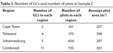
Sample B included 16 GCs with recent aerial photographs at an acceptable resolution. Sample B represented 1 813 different household plots in the 16 GCs. The GCs in Sample B are located in the Cape Town region, Johannesburg and Tshwane (Pretoria). Table 2 summarises the number of GCs and plots in each region for Sample B. The GCs in Sample B were initially selected based on available water consumption records; however, after filtering the data it became apparent that some of the GCs in Sample B contained numerous zero-consumption months. Therefore, a subset of Sample B, containing the 11 GCs with sufficient water consumption records, was selected. Table 3 summarises the number of GCs and plots in each region for Sample C.

 

 

 

 

No effort was made to target homogeneous or similar types of properties or GCs beyond the definitions provided earlier, in any of the regions. The intention was to include a variety of housing types and different types of GCs in each of the three sample sets (A, B and C) and for different regions, but this was not always possible. All relevant data that could be obtained were included in this study. For example, double-story cluster-homes were also included in some cases, with relatively small plot areas and relatively small gardens, compared to free-standing homes. However, it is acknowledged that the available data placed various limitations on the results, and that further research is needed to better classify the types of homes and GCs.

Data analyses

GCs are known to have predetermined architectural guidelines, prepared by consultants on behalf of the HOA. The architectural guidelines contribute to the aesthetics of the homes and landscaped areas of a GC. The intent is that an architectural character is developed as part of the GC's identity (Stubblefield, 1996). As part of this research, the architectural guidelines developed specifically for the 21 GCs in Sample A were obtained and reviewed. The architectural guidelines of some GCs are published online. The guidelines reviewed in this study were sourced from the relevant GC websites and subsequently examined. The review focused on attributes such as property area, building footprint area, garden footprint area, type of vegetation and pool specifications.

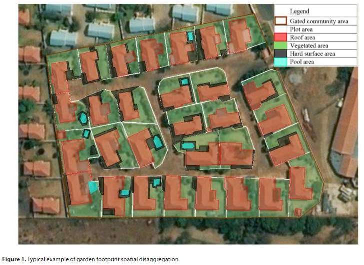
Sample B contained a different set of GCs, as described earlier. Aerial photographs of all GCs in Sample B were analysed visually to delineate the garden footprint area of all homes in the sample. The type of cover, e.g., pervious versus non-pervious or vegetated versus non-vegetated, was not further differentiated. The aerial photographs of 1 813 households in the 16 GCs in Sample B were analysed using Autodesk Civil 3D software. The Civil 3D program polygon tool was employed to measure irregular shaped objects and calculate the footprint area of property boundaries and various plot sub-areas. Each GC home was analysed individually. The surface areas of the plot, roof, vegetation, hard surface and pool were visually identified from the electronic aerial photograph image, with each type of land cover subsequently traced by adding polygons. The area of each polygon was determined and linked to the cover type per plot (an example is shown in Fig. 1). The plot area was taken as the total area within an external wall or boundary, including the driveway, verge and garage area. The garden area included the lawn and any vegetation or tree cover within the property boundary (excluding bare soil, which was added separately).

Results of architectural guideline review (Sample A)

The architectural guidelines in Sample A ranged in plot size and number of plots to enable a representative view of the housing typology. With reference to Table 4, the GCs in Sample A had 611 homes on average, while the average plot size was 783 m². The typical values specified in the guidelines were a maximum building coverage of 50% and an average minimum building floor area of between 150 m² and 250 m².

Nine of the 21 guidelines in Sample A prescribed the lawn grass genotype. The prescribed varieties included buffalo grass, kweek grass, common russet, giant spear grass, paspalum grass and Bermuda grass. Three GC guidelines stated specifically that kikuyu grass is not allowed. Of the guidelines investigated, 16 stated that no invasive plants would be permitted, 13 of which prescribed either water-wise and/or indigenous plant genotypes.

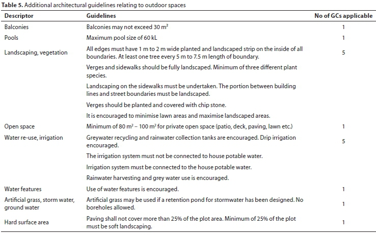
In three cases the minimum number of plants or trees per plot were recommended. In addition to plot coverage restrictions, the guidelines in Table 5 were also of interest.

Spatial analysis results (Sample B)

The prescribed spatial arrangements were compared to actual spatial arrangements of GC homes as part of this study. The aerial photographs of the 16 GCs in Sample B were analysed spatially to determine how the individual plots are developed in relation to vegetation, pool, and hard surface coverage. The GC were then classified into different regions, namely Cape Town and surrounds, Tshwane and Johannesburg. A summary of the average plot area, garden area, and percentage garden area of all the plots combined, and of the plots according to region, is presented in Table 6.

 

 

The plots located in the Cape Town region had larger than average plot areas (553 m²) and higher than average garden footprint percentage (41%), while the homes in Johannesburg had relatively smaller average plot areas (289 m²), although the garden footprint area percentage was relatively high (38.8%). Figure 2 indicates the frequency distribution of garden footprint area percentage, per region. A notable spread is evident, especially in the Cape Town region. This study was limited in the sense that socio-economic parameters (i.e. household income, property value) were unavailable due to ethical constraints. Also, the different sample sizes in the three regional sub-sets were not the same. No inference could thus be drawn regarding the relationship between garden footprint area and other independent variables. The results presented in Fig. 2 underline the differences in garden cover per region, but do not suggest region as predictor of garden footprint area.

Water use analysis results (Sample C)

The average annual daily demand (AADD) of the total GC was determined for each of the 11 GCs in Sample C, based on monthly water consumption for the period October 2012 to September 2014. No water consumption data were available for individual homes in any of the GCs. The data sample used in this study was not large enough to justify extrapolation of the findings to GC homes in general, nor could a valid relationship be found between variables from this sample.

The seasonal fluctuation of domestic water use is usually indicative of outdoor water use, especially gardening (Du Plessis et al, 2018). An indication of the seasonal water use was obtained by assuming, in line with earlier work (Ghavidelfar et al., 2018; Du Plessis et al., 2018), that the minimum winter consumption is indicative of indoor water use. The water requirement of plants and, in particular, grass, is often expressed as millimetres irrigated per week (McCready and Dukes, 2011; Venter and Grove, 2016). The seasonal fluctuation in water use of the 11 GCs in this sample was transformed by dividing monthly GC water use by the corresponding garden footprint area in order to express the water use in units of mm/week. The seasonal fluctuation was subsequently evaluated by subtracting the minimum monthly consumption in each case from the corresponding peak monthly consumption, as an approximation of outdoor use (Ghavidelfar et al., 2018). The analysed data for the GCs in each of the applicable cites were subsequently ranked as plotted, as illustrated in Fig. 4. The average seasonal fluctuation in water use in relation to the garden area for all of the GCs is 14.85 mm/ week, but varies between 3 mm/week and 30.9 mm/week.

 

 

The weekly irrigation reported in this study is in the same order of magnitude as values published by others: 15.8 mm/week in California, USA (Chen et al., 2015); 21 mm/week in Florida, USA, (Davis and Dukes, 2015); 47 mm/week in Florida, USA, (Maheshwari, 2016); and 35 mm/week Cape Town, South Africa (Nel et al., 2017). In some other regions with relatively low evaporation and relatively high rainfall, the irrigation may be negligible (Saeed Ghavidelfar, Asaad Y Shamseldin and Bruce W. Melville, 2018).

 

DISCUSSION

As expected, the disaggregation of garden footprint area for GC homes in three identified geographic regions compared well with peak monthly water consumption presented in earlier work for the same regions (Du Plessis and Jacobs, 2018). Homes in Tshwane had the lowest garden footprint area percentage, while homes in Cape Town and surrounds generally had relatively higher garden footprint areas. What was unexpected was that Johannesburg had larger garden footprint area percentages than Tshwane, although the Johannesburg homes had the lowest average plot size. Further research is needed to better classify the type of homes and GCs, since the results may be skewed by inclusion of dissimilar housing typologies in the different samples and regions reported on in this study.

The Tshwane homes' garden fo otprint percentage ranged between 0 and 70%, with an average of 22.9%, while the Johannesburg homes' garden footprint percentage ranged between 0% and 75%, with an average of 38.8%. The Cape Town and surrounds homes' garden footprint percentage ranged between 0% and 80%, with an average of 41.0%.

The water use of GC homes correlates with the garden footprint area as AADD increases when the garden footprint area increases. As part of a further study, the findings in this study could be implemented to model outdoor water use of GC homes.

 

CONCLUSION

A maximum building footprint area of between 30% and 60% is prescribed in the different GCs reviewed in this study, but the majority prescribed a maximum building footprint area of 50%. Although no specific reference is made to maximum garden footprint area, the vegetation genotype is specified in some cases, often to encourage indigenous plants, or to prevent plant genotypes that require extensive watering.

The garden footprint area of GC homes is notably influenced by total plot area and varies notably by geographic region. The average garden footprint area in relation to the total plot area was found to be 36.3% for all samples, with a standard deviation of 17.5%. In cases where the garden footprint areas of GC homes were larger than 100 m², a proportional relationship was noted between the AADD of GC homes and the average garden footprint area. Based on the assumptions for seasonal analysis of Sample C, an average of 14.85 mm/week irrigation was determined, although the irrigation demand of the 11 sample GCs was uniformly spread between 3 mm/week and 30 mm/ week.

The results show that garden footprint area (% plot cover) has a relatively wide range. Further research is needed to compare water use of GC homes to non-GC homes and to understand the contribution of GC affluence to water use. Also, a larger sample size would enable analysis of GC garden area and GC water use in different regions and would help to understand how similar homes (in similar GCs) in different regions use water differently. Findings from this study could be incorporated in the parameter calibration of outdoor water use models. Results from this study provide a useful foundation for future research into modelling water use of GC homes.

 

REFERENCES

BREETZKE G, LANDMAN D and COHN K (2014) Is it safer behind the gates? Crime and gated communities in South Africa. J. Housing Built Environ. 29 (1) 123-139. https://doi.org/10.1007/s10901-013-9362-5        [ Links ]

CZESLAW P, DARIUSZ K and RADOSLAW G (2016) The water needs of urban green areas. Ann. Warsaw Univ. Life Sci. 48 (1) 13-26. https://doi.org/10.1515/sggw-2016-0002        [ Links ]

CHEN Y, MCFADDEN J, CLARKE P and ROBERTS K (2015) Measuring spatio-temporal trends in residential landscape irrigation extent and rate in Los Angeles, California Using SPOT-5 satellite imagery. Water Resour. Manage. 29 (15) 5749-5763. https://doi.org/10.1007/s11269-015-1144-2        [ Links ]

DAVIS SL and DUKES MD (2015) Implementing smart controllers on single-family homes with excessive irrigation. J. Irrig. Drain. Eng. 141 (12) 1-10. https://doi.org/10.1061/(ASCE)IR.1943-4774.0000920        [ Links ]

DU PLESSIS JL, FAASEN B, JACOBS HE, KNOX AJ and LOUBSER C (2018) Investigating wastewater flow from a gated community to disaggregate indoor and outdoor water use. J. Water Sanit. Hyg. Dev. 8 (2) 238-245. https://doi.org/10.2166/washdev.2018.125.         [ Links ]

DU PLESSIS JL and JACOBS HE (2014) Model for estimating domestic outdoor water demand of properties in residential estates. Proced. Eng. 89 967-974. https://doi.org/10.1016/j.proeng.2014.11.213        [ Links ]

DU PLESSIS JL and JACOBS HE (2015) Procedure to derive parameters for stochastic modelling of outdoor water use in residential estates. Proced. Eng. 119 803-812. https://doi.org/10.1016/j.proeng.2015.08.942        [ Links ]

DU PLESSIS JL and JACOBS HE (2018) Analysis of water use by gated communities in South Africa. Water SA 44 (1) 130-135. https://doi.org/10.4314/wsa.v44i1.15        [ Links ]

FRAGA CCS, MEDELLÍN-AZUARA J and MARQUES GM (2017) Planning for infrastructure capacity expansion of urban water supply portfolios with an integrated simulation-optimization approach. Sustainable Cities Society 29 247-256. https://doi.org/10.1016/j.scs.2016.11.003        [ Links ]

GHAVIDELFAR S, SHAMSELDIN AY and MELVILLE BW (2018) Evaluating spatial and seasonal determinants of residential water demand across different housing types through data integration. Water Int. 22 (1) 1-17. https://doi.org/10.1080/02508060.2018.1490878        [ Links ]

HOUSE-PETERS L, PRATT B and CHANG H (2010) Effects of urban spatial structure, sociodemographics, and climate on residential water consumption in Hillsboro, Oregon. JAWRA J. Am. Water Resour. Assoc. 46 (3) 461-472. https://doi.org/10.1111/j.1752-1688.2009.00415.x        [ Links ]

JACOBS HE and HAARHOFF J (2007) Prioritisation of parameters influencing residential water use and wastewater flow. J. Water Suppl. Res. Technol. 56 (8) 495-514.         [ Links ]

KAPLAN S, MYINT S, FAN W and BRAZEL C (2014) Quantifying outdoor water consumption of urban land use/land cover: sensitivity to drought. Environ. Manage. 53 (4) 855-864. https://doi.org/10.1007/s00267-014-0245-7        [ Links ]

LANDMAN K (2004) Gated communities in South Africa: The challenge for spatial planning and land use management. Town Plann. Rev. 75 (2) 151-172. https://doi.org/10.3828/tpr.75.2.3        [ Links ]

LIANG L, ANDERSON R and SHIFLETT S (2017) Urban outdoor water use and response to drought assessed through mobile energy balance and vegetation greenness measurements. Environ. Res. Lett. 12 (8) 1-9. https://doi.org/10.1088/1748-9326/aa7b21        [ Links ]

MAHESHWARI B (2016) Understanding the performance of irrigation systems around homes. J. Environ. Eng. Landscape Manage. 24 (4) 278-292.         [ Links ]

MAHHADI ALI M, SHAFIEE M and BERGLUND E (2017) Agent-based modelling to simulate the dynamics of urban water supply: Climate, population growth, and water shortages. Sustainable Cities Society 28 (1) 420-434. https://doi.org/10.1016/j.scs.2016.10.001        [ Links ]

MAKWIZA C, FUAMBA M, HOUSSA F and JACOBS HE (2018) Estimating the impact of climate change on residential water use using panel data analysis: a case study of Lilongwe, Malawi. J. Water Sanit. Hyg. Dev. 8 (2) 217-226. https://doi.org/10.2166/washdev.2017.056        [ Links ]

MAZUMDER R, SALMAN A, LI Y and YU X (2018) Performance evaluation of water distribution systems and asset management. J. Infrastruct. Syst. 24 (3) 1-24. https://doi.org/10.1061/(ASCE)IS.1943-555X.0000426        [ Links ]

MCCREADY M and DUKES M (2011) Landscape irrigation scheduling efficiency and adequacy by various control technologies. Agric. Water Manage. 98 (4) 697-704. https://doi.org/10.1016/j.agwat.2010.11.007        [ Links ]

NEL N, JACOBS HE, LOUBSER C and PLESSIS JA (2017) Supplementary household water sources to augment potable municipal supply in South Africa. Water SA 43 (4) 553-562. https://doi.org/10.4314/wsa.v43i4.03        [ Links ]

ROITMAN S (2009) Gated communities: Definitions, causes and consequences. Urban Design Plann. 163 (1) 31-38. https://doi.org/10.1680/udap.2010.163.1.31.         [ Links ]

SOEDERBERG S and WALKS A (2018) Producing and governing inequalities under planetary urbanization: From urban age to urban revolution? Geoforum 89 (1) 107-113. https://doi.org/10.1016/j.geoforum.2017.11.005        [ Links ]

STUBBLEFIELD J (1996) Using architectural design guidelines in the planned community. The Practical Real Estate Lawyer 12 (6) 83-88.         [ Links ]

VENTER M and GROVÉ B (2016) Modelling the economic trade-offs of irrigation pipeline investments for improved energy management. Water SA 42 (4) 542. https://doi.org/10.4314/wsa.v42i4.04        [ Links ]

 

 

Correspondence:
HE Jacobs
Email: hejacobs@sun.ac.za

Received: 30 September 2018
Accepted: 6 April 2020