RESEARCH PAPERS

 

Baseline adjustment methodology in a shared water savings contract during severe water restrictions - a case study in the Western Cape, South Africa

 

 

HE Jacobs^I; JL Du Plessis^I; Nicole Nel^I; S Gugushe^II; S Levin^III

^IDepartment of Civil Engineering, Stellenbosch University, Private Bag X1, Matieland, 7602, South Africa
^IIWater & Energy Saving Management, National Department of Public Works, Western Cape Regional Office, Customs House, Foreshore, Cape Town, South Africa
^IIIWater Projects in Facilities Management, National Department of Public Works, Head Office, Pretoria, South Africa

Correspondence

 

 

---

ABSTRACT

A novel method for baseline adjustment in a shared water savings contract under serious drought conditions was presented in a companion paper. The newly developed baseline adjustment method was subsequently applied to a case study, as discussed in this manuscript. The case study involved application of the method to 24 relatively complex sites, spread over the Western Cape Province in South Africa. The sites included, for example, military bases, naval dockyards, an airforce base, prison facilities, large multi-storey blocks of flats and administrative office buildings. Baseline adjustment became essential mid-contract during the serious water restrictions in Cape Town at the time. The restrictions were linked to the 'Day Zero' scenario in 2018 when water supply would potentially run out, and resulted in water savings at baseline sites that were ascribed to external factors. The study incorporated a comprehensive review of the approved baseline reports with site visits to 12 of the properties. The baseline adjustment method provided a robust means to obtain adjustments for sites with relatively limited data. The minimum data requirement was a record of monthly water consumption per site. The adjustments varied between 0% and 64% of the original baseline value for the different sites in the study sample. The relatively higher adjustments were linked to sites where outdoor irrigation and pool water use was prevalent during the baseline-setting period, but was banned during the drought. Zero adjustments were found for sites with exceptionally high leakage flows that had subsequently been repaired; leaks dwarfed actual use in these cases. The results for all 24 sites were accepted by the contracting parties as being reasonable and fair.

Keywords: baselines, shared water savings contract

---

 

 

INTRODUCTION

This paper reports on the first application of a baseline adjustment methodology (BAM) for serious drought conditions presented by Jacobs et al. (2020) as it applied to a shared water services contract (SWSC) in South Africa. All terminology in this text was adopted directly from the companion paper. The unique method for baseline adjustment was developed for specific application to various sites in the study area, where data availability (especially in the pre-intervention period) was a particular challenge. Reference to baseline adjustment in this paper is to negative adjustment only, because the case study was limited to baseline adjustment to compensate for the effects of external influence during a drought and related water restrictions. In other words, the baseline value would be reduced by implementation of the adjustment and water savings would accordingly be reduced by the adjustment.

The study was initiated after implementation of severe water restrictions in the City of Cape Town (CoCT) and the realistic threat of a 'Day Zero' scenario, when media reports claimed that all taps would possibly run dry due to depleted water resources. One of the most notable impacts of the related water restrictions, as it pertains to this study, was the complete banning of outdoor water use. However, baselines were set at a time when outdoor use was common. The reduced consumption at baseline sites was partly ascribed to factors external to the SWSC. An adjustment to baselines was thus needed. The baseline adjustment had to be determined in a relatively short span of time and with the available data, because the contracting parties were eager to arrive at acceptable adjustments in order to assess financial implications, with particular interest in the CoCT and regions that shared water resources with Cape Town.

Description of case study sites and stakeholder involvement

The SWSC relating to this study included various sites spread over the Western Cape Province, South Africa. A total of 119 baselines were reviewed. Each baseline represented a single property, or facility. These properties are called 'sites' in the remainder of this text. Each site had a unique pre-determined and approved, fixed baseline value prior to this research study, by which savings and payment to the water services company (WASCO) were determined on a monthly basis. Baselines were determined in units of kL/day, averaged over the baseline period.

The focus in this study was on application of the BAM to the most notable 24 sites in the SWSC, which were deemed relatively complex compared to the other 95 sites. Complex sites in this study had the following attributes:

•Baseline consumption QT_B > 250 kL/day

•PRV(s) were present, or had been installed as part of saving interventions

•Sites with high recorded MNF (where MNF exceeds 50% of total flow)

•Numerous water meters (>2) and/or multiple municipal accounts

•Sites where notable pipe leaks were identified in the post-baseline period and repaired by the WASCO

The 24 sites (~20% of the total number of sites) comprised ~80% of the total baseline water use in the particular SWSC. Sixteen of the 24 sites were located in the CoCT and/or linked directly to the Cape Town water supply network; 4 of the sites were located in adjacent towns sharing water sources with Cape Town, namely: Paarl (1 site), Brakkefontein along the West Coast (1) and Stellenbosch (2); the other 4 sites were spread across the Western Cape Province in the towns of Oudtshoorn (2), Knysna (1) and George (1). Various land use typologies were included in the study sample of 24 sites, including military bases, naval dockyards, an airforce base, prison facilities (also including staff residence communities), government housing complexes, large multi-storey blocks of flats, administrative office buildings, police stations, a magistrates court and a national monument.

Earlier research has noted that any SWSC may involve numerous contract partners in complex relationships (Wegelin and McKenzie, 2005). Contracting parties in a SWSC would include at least the property owner and the WASCO. The WASCO would be responsible for water-saving interventions at sites of the property owner and the subsequent financial saving due to reduced consumption would be shared between the two parties. Additional parties in a SWSC may include a funding agent, contractor, lessee, and an independent metering and verification expert. This study involved two SWSC contracting parties, namely, the South African National Department of Public Works (NDPW) as property owner and the WASCO (Re-Solve Consulting), responsible for implementation of water-saving interventions. Sites in the study sample were on lease to various South African government departments who were not contractually involved in the SWSC, but were involved indirectly regarding operational and maintenance support and access control. Lessees of sites in the sample included, for example, the Department of Justice, the Department of Defence (including the army, navy and air force) and the South African Police Service. The water services provider, typically the local municipality, was not contractually involved in the SWSC. Water meter reading and billing of consumers were exclusively handled by the local municipality. No independent metering and verification expert was contractually involved in the SWSC; metering was conducted by the local authority (municipality) and verification was conducted by the WASCO, who would follow up queries or inconsistencies regarding metering and billing directly with the local authority.

Need for baseline adjustment

After implementation of severe water restrictions in Cape Town and neighbouring towns sharing the same water sources, the need arose to urgently adjust the formerly approved baselines in the SWSC. The NDPW invited quotes from specialists to review and revise the SWSC baselines. Stellenbosch University's Institute for Water and Environmental Engineering was subsequently appointed by the NDPW to revise and adjust the baselines for water saving at the various properties of the NDPW. The BAM presented by Jacobs et al. (2020) was developed as part of the study in order to derive adjustments for all sites, given various constraints. This manuscript describes the practical application of the BAM to various sites.

 

METHODS

Factors affecting water consumption and savings

Before discussing implementation of the BAM in the case study area, an understanding is needed of the factors that influence water use and related savings. Literature suggests five main expected impacts of water restrictions on water use, applicable to this study. Each of the factors could potentially be linked to water savings, some of which may have resulted from interventions implemented by the local authority as part of water demand management and water conservation efforts. The resultant water savings could potentially be deemed external to the WASCO interventions. The key factors linked to the various sites and to the stringent water restrictions applicable to this study were price, occupancy, consumer awareness, outdoor water use and pressure.

Price: Water price did not play a role in this study, despite research clearly linking increased water price to reduced water use (Hoyos and Artabe, 2017). Water tariffs in Cape Town notably increased with increased severity of water restrictions, but the end-users (consumers) in the study sample were not subjected to the increased price. Increased water price could be considered to have no impact on water saving at NDPW sites in this case, because of the disconnect between the NDPW, who faces the water bill, and the consumer(s) using the water.

Occupancy: A positive relationship between occupancy and consumption has been reported for residential (Jacobs and Haarhoff, 2004) and non-residential (Blokker et al., 2010) sites. However, occupancy was assumed to remain constant, because no specific change in occupancy (due to the drought) was noted at any site, nor were any accurate records of occupancy available at any of the sites. At most sites the occupancy was accepted to vary somewhat with time, for example, the number of inmates in prisons, or cohort size on military training programmes. However, the longer the period of savings analysis after inception of a SWSC, the less significant is the impact of short-term unexplained variations (USDE, 2001). The SWSC duration was 7 years in the case study, so 'normal' fluctuations in water use due to occupancy were assumed to be smoothed out.

Awareness: Consumer awareness leads to reduced consumption (Wolfe and Brooks, 2017). Awareness-driven change was limited to indoor use at sites in the study area (all outdoor use was banned). It was not feasible for the team to visit bathrooms or interview consumers on the relatively large NDPW-sites to assess the water savings as a function of consumer awareness. To complicate matters even more, the WASCO has conducted awareness campaigns on all the sites in the study sample, as part of initiatives to drive down consumption (in addition to similar efforts by CoCT). The method for baseline adjustment presented by Jacobs et al. (2020) distinguished between the effect on water savings due to consumer awareness induced by the WASCO versus awareness by CoCT (and the media in general).

Outdoor use: Outdoor use was banned during the Level 6 water restrictions in CoCT. The study area is relatively dry with a mean average annual rainfall of about 500 mm/yr, and is typified by hot and dry summer periods with predominantly winter rainfall. Peak outdoor water use occurs in summer and is driven by garden irrigation. Changes in outdoor water use would be evident when comparing the post-intervention period (the serious drought and related restrictions) with the baseline period. The notably reduced outdoor use would affect the baseline adjustment and an assessment of outdoor use was required, especially at sites with garden irrigation. Du Plessis and Jacobs (2014) identified garden footprint area as one of the most notable parameters for modelling outdoor water use. Unfortunately, the baseline reports did not specify which sections of each site (or area of the site) were irrigated during the baseline-setting period. Evaluation of garden footprint area during the study - in order to assess likely irrigated area - was considered impractical, because no outdoor areas had been irrigated for the entire previous summer season. Google aerial photography was used instead to investigate the irrigated area on sites with residential gardens, focusing on the pre-intervention period. The same approach was used by Du Plessis and Jacobs (2014) to analyse outdoor use in gated communities.

Pressure: Reduced pressure has been linked to reduced real losses (Abdulshaheed et al., 2018) and to reduced consumer use (Meyer et al., 2018). Gomes et al. (2011) presented an equation to separately estimate three components of water consumption change in relation to pressure change: (i) leakage, (ii) pressure-dependent consumption and (iii) pressure-independent consumption. Two pressure-leakage exponents (N1 and N2) were used in the equation. The N1 leakage exponent is typically used to model the relationship between pressure and leakage (Lambert, 2000; Farley and Trow, 2003). Gomes et al. (2011) concluded that it is reasonable to assume N1 equal to 1 if measured values were unavailable. The value for N2, that explains the relationship between pressure and user consumption, is normally taken to be 0.5 (Lambert, 2000; McKenzie and Langenhoven, 2001) and applies to the pressure-dependent part of the consumption. In this study the pressure-leakage relationship was used to estimate pressure-induced leakage as a function of pre- and post-intervention system pressure and one known minimum night flow (MNF) value, but only in cases where MNF was unavailable in the pre- and post-intervention periods. In all cases N1 was assumed equal to 1. The impact of pressure change on consumer demand was not evaluated by means of the N2 exponent, but was instead incorporated in a baseline adjustment contribution factor, as explained shortly.

Available information for baseline adjustment

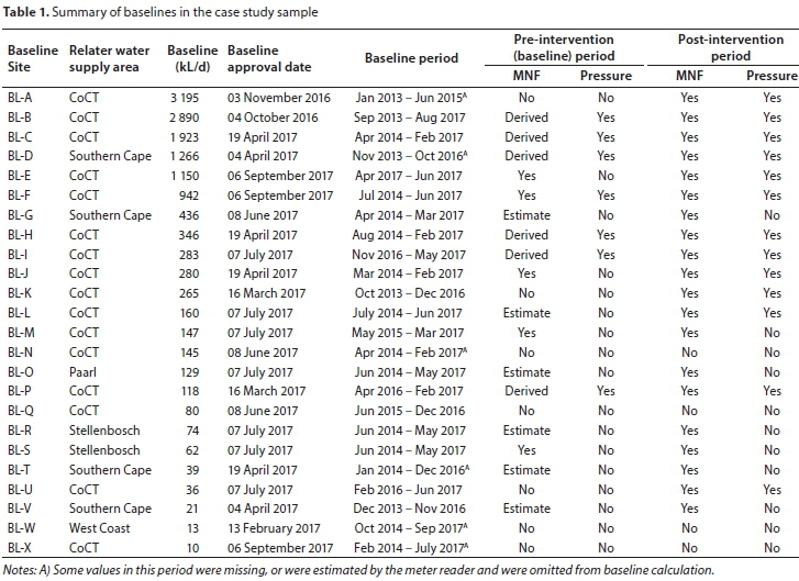
For the purpose of this paper, all site descriptions were masked by using the subscript 'BL-' (baseline) and the first 24 letters of the alphabet as site description. A list of all baselines was provided to the research team, including all relevant baseline reports, baseline calculations and the dates of baseline approval. The project team downloaded all the baseline reports relevant to the complete SWSC, which were made available via a secure OneDrive folder by the WASCO. A total of 623 files were downloaded relating to baseline reports, including related MS Excel files and PDF reports. The full dataset included 119 approved baseline reports and baseline calculation sheets, which had to be filtered to select the 24 pre-determined sites of interest.

The methodology presented by Jacobs et al. (2019) was employed to calculate adjustments for the 24 sites in the study sample. The method was based on minimum night flows in addition to monthly water consumption recorded by the local authority's (municipality's) billing system, as a basis for calculating adjustments. Earlier research in South Africa noted the value of monthly water consumption extracted from municipal billing systems (Jacobs and Fair, 2012) for research projects. Monthly water meter readings taken by the CoCT and other municipalities in the study area were available from two sources, namely the WASCO and the municipal billing system. Monthly water consumption was used in this study and was reasonably easy to obtain. In addition to monthly consumption, flow rates and pressures were recorded at some sites by means of data loggers, but were not available in all cases and were often limited to the post-intervention period. The flow rates and pressures were found to be useful in order to assess the minimum night flow (MNF) - and to obtain an indication of real water losses. Table 1 provides an overview of the 24 baseline sites and lists the integrity of MNF- and pressure-data available for each site for the pre-intervention (baseline) and post-intervention (drought) periods.

Minimum night flow

Real losses could be estimated by assessing the MNF. The validity of this assumption would vary depending on the time of day that MNF was recorded, the actual night-time consumer usage and the measurement resolution. Gomes et al. (2011) points out that MNF is linked to the period of highest pressure, when the demand is normally at a minimum. Thus, using MNF as an estimate for total daily leakage would over-estimate the leakage, especially in cases where the pressure fluctuates notably during the day as a function of demand. However, for most of the NPDW sites in this study, pressure was controlled by means of a pressure-reducing valve (PRV). The actual consumer usage was expected to be relatively close to zero at night, so the assumption of MNF rate being equal to average daily leakage flow rate was considered reasonable for all sites. The pressure-leakage relationship was used in this study to evaluate the leakage as a function of pressure change (from pre- to post-intervention periods), but only if MNF values were not available.

 

RESULTS AND DISCUSSION

Adjustments for all sites

With reference to the BAM presented in the companion paper by Jacobs et al. (2020), the adjustment calculations were linked to four unique cases, depending on data availability. The four cases are listed below in order of decreasing data availability:

•Case 1: Monthly consumption and MNF are available in both periods

•Case 2: Monthly consumption is available, plus MNF in one period and water pressure available in both periods

•Case 3: MNF is unavailable; adjustment was based on monthly consumption

•Case 4: Monthly consumption is available, but the consumption record required for Case 3 is insufficient to justify application of Case 3 (e.g. the minimum winter month was missing or estimated); MNF could be estimated in such cases by means of the REM procedure described by Jacobs et al. (2020) in a companion paper

The four cases are presented in detail in the companion paper (Jacobs et al., 2020). Table 2 shows which of the four BAM-cases applied to each site and presents the model input data. The contribution weight factors (α, β and γ) were obtained from the relevant table for these factors, presented by Jacobs et al. (2020). In Cases 1, 2 and 4, where MNF could be obtained, factor α is required; factors β and γ apply to Case 3. The contribution-factor α for Site BL-A was based on the assumption that 25% of the contribution would be from the residential settlement on the property (with α = 0.4) and 75% from the rest of the site (α = 0.8). The combined contribution factor was α = 0.7 for Site BL-A. The subsequently calculated adjustments for all 24 complex adjustments are presented in final two columns of Table 2. The baseline adjustment is presented in kL/day and as a percentage of the baseline value.

Discussion regarding Site BL-A

Application of the BAM to Case 1 and Case 2 type sites, involving MNF, was relatively uncomplicated. In cases where pressure was used to estimate the MNF, the pre- and post-PRV-intervention pressures are listed in Table 2; the pressure was equal to the recent values reported. The N1 factor was assumed equal to 1 in all sites where the pressure-leakage relationship was employed to estimate MNF. The result is relatively sensitive to change in the N1 parameter. The value for N1 = 1 was used for six of the sites, but for Site BL-A a more comprehensive site-specific approach was followed.

Site BL-A was a derelict military base, great portions of which had fallen into disuse. Despite the previous statement, Site BL-A was the largest of the sites in terms of the baseline water use. It soon became apparent that infrastructure on this site was poorly maintained and that notable water leakage and losses occurred in the baseline period. The pre-intervention leakage-evaluation at Site BL-A was complicated by numerous issues, including notable sections of pipe that were decommissioned by the WASCO (thus notable change in the total pipe length) soon after interventions started. Notable leak identification and leak repair were performed as part of initial interventions and also notable sections of unnecessary water-use points (e.g. ablution facilities) were taken out of service to further reduce leakage. Nsanzubuhoro and Van Zyl (2018) conducted an on-site pressure-leakage test on a particular section of pipe at the Site BL-A. The test was conducted at exceptionally low pressures (10 m to 30 m head) to prevent pipe bursts. An N1 value of 0.79 was reported for a short section of pipe, but the leak area (and thus leakage) was expected to increase substantially at higher pressures, with a dual linear model presented by Nsanzubuhoro and Van Zyl (2018). The slope of the linear model, with pressure on the x-axis and flow rate on the y-axis, increased substantially from 0.93 for pressures below 1.8 bar to 7.36 for pressures exceeding 1.8 bar. The linear equations presented by Nsanzubuhoro and Van Zyl (2018) only describe the change in leak area (not actual leakage) with pressure; notably higher leakage rates were expected at higher pressures, as would have been experienced during the baseline period.

Also, Site BL-A comprised sectorally mixed land use, each typology with notably different character in terms of leakage and water use, and different supply points with different supply pressures and unsynchronised PRV pressure changes in the transition period from pre- to post-intervention. An attempt was made to estimate leakage based on average pressures, but the results were unsatisfactory. The combination of these issues justified a detailed investigation for estimating the MNF at Site BL-A, instead of using the pressure-leakage relationship directly. A detailed evaluation of baseline adjustment calculation for Site BL-A was subsequently conducted.

Site BL-A was visited on 12 July 2018 to obtain the necessary on-site information and to observe the potential water use influences. The site comprised a residential community, a tertiary training college, large military stores, various administrative buildings in everyday use and also large portions of derelict abandoned military facilities (including also a disused airfield, barracks and stores). The site was analysed theoretically to estimate the water use and real loss in the pre-intervention period.

In order to achieve the pre-intervention flow pattern, it was necessary to understand the expected water use of consumers on the site. Fortunately, the flow rate and pressure at all supply points to the site were recorded constantly in the post-intervention period. The flow pattern was considered to comprise three main components, namely indoor use (from the military base, a training college and the residential homes), outdoor use (mainly the residential homes and communal gardens) and leakage (all sections of the site). These three components were not metered separately. The model is described in Eq. 1:

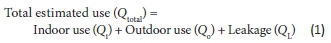
where the indoor use was expected to not have been influenced by water restrictions, because of the nature of the site and the fact that the end-consumers do not pay for water use. The indoor water use (assumed equal for pre- and post-intervention periods) was derived from recently recorded water flow rates, at both supply connections separately. The indoor water use was estimated by subtracting the average post-intervention MNF from the average post-intervention total flow rate at each connection point, as summarised in Table 3.

 

 

For the residential community, which was fed from the western supply point, the following equation presented by Du Plessis and Jacobs (2014), was used to model the outdoor use:

where

Q_outdoor= Outdoor water demand

A_i = The area of a property that is under irrigation

E_to = Evapotranspiration

K_bc = Crop coefficient

P_r = Measured precipitation

F_ep = Effective Precipitation Factor

I_e = Irrigation efficiency

A_p = The surface area of a pool or water feature

E_w = Open lake evaporation rate of water (including pan factor)

P_r = Measured precipitation

D_d = The water level difference after performing a maintenance cycle

A_p = The surface area of a pool or water feature

O_m = The occurrence of pool maintenance per calendar month

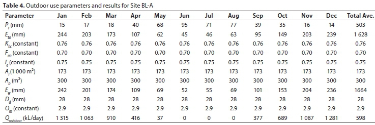
Using aerial photography, the parameters such as garden area and pool area for the outdoor use were derived, as illustrated for one section of the site in Fig. 1. The remaining parameters were obtained from other sources, including the Department of Water and Sanitation (refer also to Du Plessis and Jacobs, 2015). The input parameters used for modelling the outdoor use are summarised in Table 4. Equation 2 was used to theoretically estimate the outdoor use component. The results for outdoor use are also presented in Table 4.

 

 

The total theoretically derived baseline consumption, including estimated garden irrigation in the pre-intervention period, is found by adding the components (162 + 598 = 760 kL/d). The value of 760 kL/d represents the best estimate of actual consumption in the pre-intervention period, but excludes real losses. The MNF in the baseline period could be estimated by subtracting the estimated water use by consumers (760 kL/d) from the total baseline consumption (3 195 kL/d). The estimated real loss in the baseline period was thus 2 435 kL/day, based on annual averages.

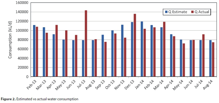
The water consumption could be estimated for each month, and could be compared to actual water consumption of the site on a monthly basis, as illustrated in Fig. 2. The outdoor end-use model was not calibrated in this case, because outdoor water use was not measured separately. Generally, good agreement was apparent between the modelled and measured data for the whole site in most months. Considering that the baseline adjustment was based on an annual average, and other relatively crude input variables, the model result was considered acceptable and was used instead of a pressure-leakage estimate.

The impact of MNF on adjustments

Relatively high MNF values, in relation to typical reports from developed countries, were found at most sites. Figure 3 presents a ranked plot of MNF in the pre-intervention period for the 18 sites for which MNF could be determined. The MNF ranged from 7% to 93% of the pre-intervention baseline consumption, with MNF at 5 sites exceeding 80% of baseline consumption. Four of the values in Fig. 3 represent MNF that were derived as per Case 4 and were not measured directly (BL-G, BL-O, BL-T and BL-V). The reduction in MNF from the pre- to post-intervention period is also presented in Fig. 3, for all 18 sites with MNF. The highest value of 2 231 kL/d was reported at Site BL-A, which was also the site with the highest baseline consumption.

 

 

Baseline adjustments varied notably from one site to the next, with a wide range of adjustment values when expressed as percentage of the baseline value. Two of the sites presented in Fig. 3 reported no change in MNF, while water savings interventions had resulted in MNF reduction at the remaining 16 sites. For these 16 sites the contribution of MNF to the total water saving was compared to the adjustment values, as presented in Fig. 4. The adjustment is expressed as a percentage of the baseline consumption. The x-axis in Fig. 4 presents parameter x as the reduction in MNF divided by the total consumption change from pre- to post-intervention period, thus providing insight into the contribution of the MNF change to the total water saving at each site. In four of the cases, the MNF change represented the total change in consumption (all four points plot at 100% on the x-axis and 0% on the y-axis).

 

 

Envelopes added to Fig. 4 illustrate the narrowing range in adjustments found with increased MNF contribution at the 16 study sites. The linear fit to the data, presented in Eq. 3, provides an R² value of 0.77, suggesting that 77% of variance could be explained by the relatively basic linear model; the line was not forced to pass through the expected x-axis intercept of (100, 0). Further analysis of the data shows an adjusted R² of 0.75, accounting for the sample size (16) and number of independent variables (1) in the model. The linear model for adjustment (y) based on MNF contribution (x), with both parameter values expressed as a percentage, is:

Despite the relatively good correlation presented by the single parameter model (Eq. 3), baseline adjustment is clearly sensitive to the type of site. The study area included various different types of sites, as listed in Table 2. Consider the following two examples, assuming for the moment equal influence of MNF at both sites: first consider a residential settlement with notable garden irrigation in the baseline period, followed by the irrigation ban during restrictions in the post-intervention period - clearly the baseline adjustment would be relatively high to compensate for the external influence (non-WASCO) regarding water saving; in contrast, consider (say) a prison facility with no gardening and inmates that are unconcerned with water saving - the baseline adjustment would be relatively low because any possible saving at the site would likely be due to interventions by the WASCO. However, the limited sample size of this study did not allow for additional parameters to be included, or different models to be developed for each site typology.

 

CONCLUSION

A novel method for baseline adjustment, presented by Jacobs et al. (2019), was successfully implemented in a South African case study despite various constraints regarding data availability. Baseline adjustments were derived for all 24 sites by considering 4 adjustment cases, each of which allowed for different layers of data integrity. Adjustment calculation is aided by knowledge of the minimum night flows in the pre-intervention period (it is typically possible to record the MNF in the post-intervention period when adjustments need to be calculated). The robust method allowed for adjustments to be determined - in the absence of recorded data - by implementing assumptions to assess water use and related savings at relatively complex sites. Contribution to savings could be evaluated by implementing weight factors, which could be agreed on between the contracting parties. The BAM and various input parameters could find potential application in practice, say by including the said procedures in the procurement process of future shared water savings contracts.

 

ACKNOWLEDGEMENTS

The research results presented in this report emanate from a contract research project conducted by Stellenbosch University for the National Department of Public Works, South Africa. The methodology presented in this paper was the outcome of valuable collaboration between the Stellenbosch University project team and all stakeholders at the NDPW, Re-Solve and the City of Cape Town.

 

REFERENCES

ABDULSHAHEED A, MUSTAPHA F and ANUAR M (2018) Pipe material effect on water network leak detection using a pressure residual vector method. J. Water Resour. Plan. Manage. 144 (4) 05018006-1 - 05018006-10. https://doi.org/10.1061/(ASCE)WR.1943-5452.0000798        [ Links ]

BLOKKER EJM, VREEBURG JHG and VAN DIJK JC (2010) Simulating residential water demand with a stochastic end-use model. J. Water Resour. Plan. Manage. 136 19-26. https://doi.org/10.1061/(ASCE)WR.1943-5452.0000002        [ Links ]

DU PLESSIS JL and JACOBS HE (2014) Model for estimating domestic outdoor water demand of properties in residential estates. 16^th Conference on Water Distribution System Analysis (WDSA 2014), 14-17 July 2014, Bari, Italy. Procedia Eng. 00 (2014) 000-000 1-8.         [ Links ]

GOMES R, MARQUES AS and SOUSA J (2011) Estimation of the benefits yielded by pressure management in water distribution systems. Urban Water J. 8 (2) 65-77. https://doi.org/10.1080/1573062X.2010.542820        [ Links ]

HOYOS D and ARTABE A (2017) Regional differences in the price elasticity of residential water demand in Spain. Water Resour. Manage. 31 (3) 847-865. https://doi.org/10.1007/s11269-016-1542-0        [ Links ]

JACOBS HE, DU PLESSIS JL, NEL N, GUGUSHE S and LEVIN S (2020) Baseline adjustment methodology in a shared water savings contract under serious drought conditions. Water SA 46 (1) xxxxx.         [ Links ]

JACOBS HE and HAARHOFF J (2004) Structure and data requirements of an end-use model or residential water demand and return flow. Water SA 30 (3) 293-304. https://doi.org/10.4314/wsa.v30i3.5077        [ Links ]

MEYER N, JACOBS HE, WESTMAN T and MCKENZIE RS (2018) The effect of controlled pressure adjustment in an urban water distribution system on household demand. J. Water Suppl. Res. Technol. 67 (3) 218-226. https://doi.org/10.2166/aqua.2018.139        [ Links ]

USDE (United States Department of Energy) (2001) International Performance Measurement & Verification Protocol. Concepts and Options for Determining Energy and Water Savings. Volume I. International Performance Measurement & Verification Protocol Committee, January 2001. DOE/GO-102001-1187.         [ Links ]

WOLFE S and BROOKS D (2017) Mortality awareness and water decisions: A social psychological analysis of supply-management, demand management and soft-path paradigms. Water Int. 41 (1) 1-17. https://doi.org/10.1080/02508060.2016.1248093        [ Links ]

 

 

Correspondence:
HE Jacobs
hejacobs@sun.ac.za

Received: 23 October 2018
Accepted: 15 November 2019