RESEARCH PAPERS

 

Baseline adjustment methodology in a shared water savings contract under serious drought conditions

 

 

HE Jacobs^I; JL Du Plessis^I; Nicole Nel^I; S Gugushe^II; S Levin^III

^IDepartment of Civil Engineering, Stellenbosch University, Private Bag X1, Matieland, 7602, South Africa
^IIWater & Energy Saving Management, National Department of Public Works, Western Cape Regional Office, Customs House, Foreshore, Cape Town, South Africa
^IIIWater Projects in Facilities Management, National Department of Public Works, Head Office, Pretoria, South Africa

Correspondence

 

 

---

ABSTRACT

Baselines are often employed in shared water saving contracts for estimating water savings after some type of intervention by the water service company. An adjustment to the baseline may become necessary under certain conditions. Earlier work has described a number of relatively complex methods for baseline determination and adjustment, but application in regions faced with relatively limited data becomes problematic. If the adjustment were determined before finalising the contractual matters, it would be possible to gather the required data in order to determine the adjustment. However, in cases where no adjustment was fixed prior to the contract, a method is required to determine an adjustment mid-contract based on whatever data are available at the time. This paper presents a methodology for baseline adjustment in an existing shared water savings contract and explains how adjustment could be determined mid-contract, under conditions of limited data. The adjustment compensates for expected reduced water consumption due to external influences induced by serious water restrictions, typically introduced during periods of drought. The fundamental principle underpinning the baseline adjustment methodology presented in this paper involved segregating real water losses from the actual consumption of end-users, preferably by analysing the minimum night flow. In the absence of recorded night flows, an alternative procedure involving the minimum monthly consumption pre- and post-baseline was employed. The baseline adjustment method was subsequently applied in a South African case study, reported on separately. This technique is helpful because adjustments could be determined without adding unnecessary complexity or cost, and provides a means to resolve disputes in cases where unexpected savings occur mid-contract.

Keywords: baselines, leakage, shared water savings contract

---

 

 

INTRODUCTION

Various terms are used when referring to a shared energy savings contract, including risk-reward contract, energy savings contract, shared energy contract, performance contracts, and many more. In this text the term 'shared water savings contract' (SWSC) is used. In a SWSC the savings achieved after interventions by the water services company (WASCO), and thus related payment to the WASCO, are measured against some pre-determined baseline value, often called a base year.

Earlier research has noted that any SWSC may involve numerous contract partners in complex relationships (Wegelin and McKenzie, 2005). The SWSC would include at least two contracting parties, namely the property owner and the WASCO. Parties may include a funding agent and an independent expert to adjudicate savings, in addition to the owner and the WASCO.

Water and energy savings are often viewed integrally (and reported on in this manner in literature) when savings and related contractual matters are concerned. The use of a baseline for estimating savings in a SWSC after some type of intervention by the WASCO is common. Some baselines are contractually fixed, while others allow for pre-determined adjustments over time. USDE (2001) comprehensively explained baseline adjustments. The adjustments could be steady (for example a monthly increase to allow for steady growth in an area) or could allow for any other conditions that commonly affect water use (e.g. weather). Also, adjustments could be positive, allowing for an increased baseline value due to explainable increased water use over time, or the adjustment could be negative to compensate for savings that are external to the SWSC, thus cannot be ascribed to interventions by the WASCO. This study exclusively involved negative adjustments, allowing for reduced consumption over time (relative to normal conditions) due to serious water restrictions that were implemented during a drought.

According to USDE (2001), baseline adjustments are derived from identifiable physical facts, which implies that these adjustments could be measured and would be included in the SWSC. Adjustments could be made routinely, or when deemed necessary in the light of physical changes. Allowance for adjustments in a SWSC are the most complicated component of setting up the baseline contract, because description of the adjustments relies heavily on the availability of accurate data for numerous parameters, all of which must be routinely measured to assess savings. The required data intensity and accuracy in developing countries may not be available and a SWSC may take a simpler form, say by assuming a fixed baseline value.

Consideration for adjustment

An adjustment to baselines becomes necessary under certain conditions. Negative adjustment would be required to compensate for water savings that are not necessarily ascribed to initiatives introduced by the WASCO. The saving may have resulted from external factors, which led to reduced water use at a particular site, for example:

•Pressure reduction in the upstream supply system by the water service provider, particularly in the absence of pressure reduction by the WASCO

•Water restriction measures that target specific end-uses, such as garden irrigation, or banning of all outdoor water use

•Increased cost of water faced by the end-user (consumer), as increased cost is known to reduce consumption

•Decommissioning certain sections of the site

•Consumer awareness campaigns that may lead to changed habits, such as shorter showers, reduced toilet flush frequency or in-house greywater reuse

Positive adjustment would result from external factors that increase water use at a particular site and could be considered to be beyond the control of the WASCO, for example:

•Increased occupancy over time

•Construction of new building(s) on the site

•Refurbishment of building(s) on site in view of land use change, e.g., densification

•Increased commercial or other day-to-day activity on a site

•Weather fluctuations (including climate change) that may lead to increased outdoor irrigation needs with increased temperatures and reduced rainfall over time

Research question

How could the baselines in an existing shared water savings contract be adjusted, under conditions of limited data, to compensate for expected reduced water consumption due to external influences caused by emergency water restrictions?

Scope and limitations

A unique method of baseline adjustment is presented in this paper for application to cases where no adjustment was recorded in the SWSC, but consumption was notably reduced by external factors, resulting in the need for an adjustment mid-contract. The method presented in this paper was aimed at regions with limited data, relative to what is typically required for savings determination and baseline adjustments reported on elsewhere (USDE, 2001).

The methodology derived as part of this study was based on the assumption that data would be limited to at least monthly water consumption records, available for a notable portion of the baseline period. Monthly records sufficient for setting a baseline would be available (else, there would be no grounds for a baseline). More accurate flow records - providing insight into minimum night flow - would be available for selected ad-hoc periods in at least the post-baseline period. The latter would typically be the result of measurements by the WASCO at pressure control valves or at additional water meters, as part of water-saving interventions and periodic inspections.

Terminology

Notation used in this text was adopted mainly from Gomes et al. (2010) and is in line with earlier reports by Lambert (1994) and May (1994) and related water balance terminology by the International Water Association (IWA).

 

METHODS

Baseline determination

When setting up baselines, 'It is better to complete a less accurate and less expensive savings determination than to have an incomplete or poorly done, yet theoretically more accurate determination ...' (USDE, 2001 p. 21). Use of existing meters is common for baseline setting and savings determination, but literature underlines the value of a third party to help compile baselines and to assess reported savings on a regular basis. Third parties are typically needed when the firm performing the savings has more experience than the property owner does. Some methods rely on separate measurements of parameters (e.g. different buildings on a site or separate components of the usage profile) instead of a single measurement for the whole site. Also, parameters for baseline determination and savings calculations could be continuously measured or periodically measured. The separate measurements are then factored together to determine the baseline, or compute the saving. However, if baseline determination relies on consumption reported by existing water meters, then segregation of usage components is impractical and the parameters are recorded periodically (i.e., when water meters are read by the service provider). The WASCO is unlikely to risk investment, say to record additional water use at high resolution for separate components, prior to having the baseline approved. Also, the property owner may not intend investing for this purpose. Added complexity in baseline and savings determination typically involves added cost to evaluate additional parameters needed to determine the savings (e.g. the need to count people on the site at regular intervals; measurement of weather variables; an assessment of actual expenses by the WASCO and so forth).

Corbett et al. (2005) described shared-savings contracts as having a fixed service fee with a variable component based on consumption volume. The same authors describe a broader class of cost-of-effort functions than the linear cost-of-effort functions commonly found in practice. Linear cost-of-effort functions are applicable to this study and relate the reward (payment to the WASCO) in a linear fashion to the effort (savings by the WASCO). Corbett et al. (2005) also show that small changes in the problem parameters could notably affect profits, suggesting that the selection of parameters is important. The most basic parameter in the relationship would be water savings, e.g., a single consumption value based on a metered connection.

Rossi et al. (2014) used a relatively complex method for baseline determination of energy consumption by employing artificial neural networks to recreate the post-retrofit consumption; the work is not directly applicable to this research, because the input data in this study lacked the required accuracy and also the post-retrofit water consumption would typically be measured directly.

The longer the period of savings analysis after inception of the SWSC, the less significant is the impact of short-term unexplained variations. A duration of 5 to 10 years would smooth out normal fluctuations in water use.

Water consumption and savings estimation

Two notably different components of the total water use profile were considered in this investigation, namely water consumption (the actual usage by end-users) and water losses. At each facility, the flow volume of both components combined would be metered, and the consumer would normally be billed for both in the same manner and at the same tariff. This section provides a concise review of methods for estimating the actual consumption, followed by matters relating to water loss.

Models for estimating water demand abound, and a comprehensive discussion of the methods and models was considered beyond the scope of this study. A number of commonly employed methods for estimating water use locally were based on empirical data (CSIR, 2003; Jacobs et al., 2004; Jacobs et al., 2013). Also, Jacobs and Haarhoff (2004) presented a theoretical end-use model for household water use called REUM, that was further extended to include stochastic variables (Scheepers and Jacobs, 2014). Independently, Blokker et al. (2010) developed a similar stochastic model called SIMDEUM which allowed for increased temporal resolution.

A model for estimating outdoor water use was developed by Du Plessis and Jacobs (2015). Various advanced methods are also available elsewhere to estimate the water demand of consumers, including comprehensive end-use studies (Beal et al., 2011; Mayer et al., 2003; Arbon et al., 2014). Advanced algorithms such as genetic algorithms (Di Nardo et al., 2015) are available to minimise the deviation between predicted and measured time-series data at hourly intervals.

Pressure reduction is often reported as the fundamental step towards water savings, because reduced pressure leads directly to reduced real losses (Schwaller and Van Zyl, 2014; McKenzie, 2002; McKenzie et al., 2003), but could also result in reduced demand (Meyer et al., 2018). The impact of pressure reduction on water savings is more notable in cases of high leakage prior to intervention. The pressure-leakage relationship is well documented (Van Zyl and Malde, 2017; Gomes et al., 2011; Lambert (2002). International best practice centres around the so-called 'IWA Water Balance', where different components of leakage are described, including current annual real loss (CARL), unavoidable annual real loss (UARL) and the infrastructure leakage index (ILI). The minimum night flow (MNF) usually occurs between the hours of 02:00 and 04:00 (Mutikanga et al., 2013) and is useful for estimating leakage in water distribution system zones (Cheung et al., 2010). The MNF provides an accurate estimate of the real losses in a distribution system, provided that the zone is discrete (there is no cross-boundary flow into or out of the zone that is measured) and provided that the actual consumption during certain night hours is negligible. The MNF is a function of water pressure, with reduced pressure resulting directly in reduced MNF.

Water pressure notably affects water loss, but also influences the actual demand of users. The well-documented pressure-leakage relationship (Lambert 2002; Gomes et al., 2011; McKenzie, 2001; McKenzie et al., 2002) involves a theoretical procedure to evaluate leakage reduction due to reduced pressure by incorporating the so-called N1-exponent, which is explained by Gomes et al. (2011). Water distribution system pressure is typically reduced by installation of pressure-reducing valves, keeping in mind that the minimum pressure at the critical point in the system needs to meet certain operational criteria (Strijdom et al., 2017). Gomes et al. (2011) presented a method to assess the benefits of pressure management and to evaluate the cost-benefit of pressure reduction efforts. Meyer et al. (2018) investigated demand reduction due to reduced pressure in an operational WDS in South Africa and presented a linear relationship, based on relatively crude data from the field investigation.

Water loss from leaks and bursts can be calculated using software, such as PrimeWorks software (Alkasseh et al., 2015) and the locally developed Benchleak and Presmac software suites (Seago et al., 2004; McKenzie, 2001; McKenzie et al., 2002). Software tools typically rely on accurate input data, which may not necessarily be available. Methods have also been developed for detecting leakage based on statistical analysis of actual consumption data (Buchberger and Nadimpalli, 2004), but the methods only apply to small residential service zones. The work shows that it is possible to evaluate leakage based on consumption data - a principle that was also applied in this study.

Gomes et al. (2011) presented an equation to estimate the total consumption QT₁ (thus for leaks and actual use) for the pre-intervention state and the post-intervention state. The N1 leakage exponent is used to model the relationship between pressure and leaks, as per the model by Gomes et al. (2011), with N1 typically assumed equal to 1. The N2 exponent in the same model explains the relationship between pressure and user consumption. The value for N2 is normally taken to be 0.5 (Giustolisi et al., 2008; Gomes et al., 2011), but applies only to the pressure-dependent part of the consumption. The pressure-dependent and pressure-independent components of water use in each building on each site would have to be estimated in order to employ the Gomes et al. (2011) equation.

The leakage flow QL₀ could be estimated by assuming that the daily leakage flow (say hourly) would be equal to the MNF (volume per hour). This reference to 'daily leakage flow' would vary depending on what time of day it is referring to, how it is calculated and over what period of time. As used in this study the term is used in a general sense to describe the average leakage flow over 24 h, for the period under consideration (e.g. the baseline period, or maybe a recent post-intervention week). MNF is linked to the period of highest pressure, when the demand is at a minimum. Thus, using MNF as an estimate for total daily leakage would overestimate the leakage, especially in cases where the pressure fluctuates notably. However, when pressure is controlled (as was the case for most of the NPDW sites) the assumption of MNF rate being equal to average daily leakage flow rate is more valid.

The leakage-pressure relationship was used in this study to evaluate the changed leakage and consumption after changes in pressure if the following were known: MNF before change, pressure before change, pressure after change and consumption before change. These values could be obtained for most of the complex sites in this study, although in some cases the MNF before change would have to be estimated where necessary.

Of course, the calculation is only needed for those cases where pressure management upstream induced pressure change impacts on the particular baseline site directly. In cases where pressure changes due to WASCO initiatives apply in the absence of upstream pressure initiatives, this calculation would not be needed - all the pressure-induced savings would be due to the WASCOinitiatives.

Development of baseline adjustment methodology

The baseline adjustment methodology for drought conditions was developed in parallel with application on selected sites as part of a pilot project and was subsequently implemented in South Africa (Jacobs et al., 2020). The application showed that the method was practical and could be implemented for baseline adjustment at various levels of data integrity and availability. A phased approach was needed, using the most accurate data if available, else shifting to an alternative less accurate method. The fundamental principle underpinning the baseline adjustment methodology involved segregating the total consumption into two components: (i) real water losses and (ii) the actual consumption of end-users. The two water use components would allow different contributions to be allocated to the WASCO efforts (versus external factors) in each case.

The approach is best described by considering Fig. 1. Keep in mind that Period B represents the baseline period, while Period m would be any (much later) post-intervention period. Typically, the real water loss would have been reduced in Period m, when compared to Period B. The water saving from Period B to Period m is due to reduction in the real loss-component (depicted as reduced MNF from Period B to Period m in Fig. 1) plus the reduced consumption component. The consumption component change is equal to the difference between the total use, QT_B, and real loss, QT_L, in Period B, and the difference between the total use, QT_m, and real loss, QT_m,,in Period m. This principle was used to derive the equation for baseline adjustment when MNF was known, but an alternative was needed in cases where the MNF was not known and could not be estimated.

 

 

The adjustment calculation relies on the assumption that the MNF is a realistic representation of real losses in the system in both periods, or MNF_B = QL_B and MNF_m = QL_m. Change in the leakage term is considered to be due to interventions by the WASCO, especially if pressure is managed by the WASCO at the particular site. The change in the actual end-user consumption is both due to the WASCO interventions and external factors, which have to be shared in a sensible manner. The latter was handled by introducing a factor to describe the contribution by the WASCO.

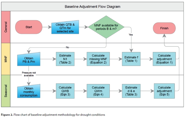
The baseline adjustment methodology is presented as a flow chart in Fig. 2. The necessary inputs include the total monthly consumption (kL/d) during the baseline period QT_B as well as the total monthly consumption for the post-intervention period in question, which is termed QT_m. The method was split into three (horizontal) tiers, as illustrated in Fig. 2. The three tiers could broadly be described as follows:

•General: Data input and general processes

•MNF: The actual minimum night flow, based on recorded flow rate, is used as a proxy for real losses; the adjustment would be based on actual data, or in the absence of one MNF value a secondary step is needed whereby MNF is derived from pre- and post-intervention system pressure

•Seasonal: The minimum winter month consumption is used to evaluate the base flow, which would include leakage

 

RESULTS

Baseline adjustment

Adjustment calculation

The general equation for baseline savings in a shared water savings contract (SWSC) is presented by USDE (2001) as:

The water saving for month m, QS_m, is equal to the total baseline water use, QT_B, minus water use of the current month, QT_m. In a SWSC with no adjustments the water saving in month m is calculated with Eq. 2:

Assuming that negative adjustments have to be incorporated, the water saving for month m becomes:

The challenge is to calculate a scientifically based adjustment value for any SWSC, given the data restrictions mentioned earlier. With reference to the flow diagram presented in Fig. 2, three alternative routes are subsequently presented. The adjustment calculations for the three methods are based on decreased data availability in each case:

•Case 1: Monthly consumption and MNF are available in both periods

•Case 2: Monthly consumption is available, plus MNF in one period and water pressure available in both periods

•Case 3: MNF is unavailable and the adjustment has to be based exclusively on monthly consumption

Ideally, 12 adjustment values would be calculated, one per month, in line with reported savings calculations in literature (USDE, 2001). However, in view of limited monthly consumption data, 12 unique monthly adjustment values were not deemed achievable. Adjustment could possibly be stepped for 4 seasons, instead of 12 adjustments, one for each month. However, seasonal adjustments were considered impractical due to data limitations and the model was constructed based on an annual adjustment value. One adjustment value is determined per site (thus per baseline) with the baseline adjustment methodology presented in this paper; the adjustment would apply for the duration of the serious water restrictions.

Case 1: MNF available in both periods

The method for baseline adjustment is explained by considering the most basic case first, presuming that MNF is available in both periods. Total monthly water use (kL/d) and MNF (kL/d) should be available for the baseline period and also for the post-intervention period. The MNF could involve any measurement during the baseline calculation period that is deemed representative of the baseline period, along with a recent measurement. Ideally the MNF should be recorded for each month to be invoiced, but the method is applicable if any representative MNF value is available in both periods. A representative MNF value could possibly be derived from only a few days of ad-hoc data recording, if conditions on the site (including leakage rates) remain quite static.

The parameters needed to follow Route 1 include the total monthly consumption for all months in the baseline period, QT_B, the current monthly consumption for the recent month, QT_m as well as MNF for the two periods. In the absence of an adjustment the savings QS would be calculated by comparing QT_B and QT_m as per Eq. 2. As explained earlier (refer to Fig. 1), the water savings QS* could alternatively be calculated for the two different water use components separately by introducing a contribution factor α and by assuming that MNF is a good representation of real losses. Equation 4 is used as an alternative to calculate the water savings, QS*:

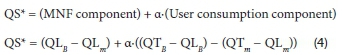
The contribution factor α is used to explain which fraction of use is ascribed to the WASCO, versus external influences. Equation 4 correctly simplifies to Equation 2 in the case where α = 1. Values for the contribution factor α are presented in Table 1, with limits of α = 0 for the case where the WASCO has no contribution to savings and α = 1 in the extreme of exclusive WASCO-induced savings. The values for α relate to the type of baseline sites forming part of a South African case study, reported on separately (Jacobs et al., 2020).

The adjustment parameter included in Eq. 3 must equal the difference between the original QS calculation in Eq. 2 and the adjusted QS* given in Eq. 4. Some margin of error, say ε, is introduced by the assumptions stated earlier and due to measurement of the MNF. In other words, the adjustment is found by Eq. 5:

Assuming that ε is relatively small compared to the errors known to exist in monthly consumption data, and also assuming that ε is relatively small compared to the baseline adjustment value, the error term was ignored. The baseline adjustment is found by Eq. 6, by substituting Eqs 2 and 4 into Eq. 5. Equation 6 is used to calculate the adjustment of the baseline (in kL/day) for cases with MNF in both periods:

Case 2: MNF available only in one period

Ideally, a representative measured MNF is needed for the baseline period and the post-intervention period, as considered in Case 1. However, the real losses could be estimated if MNF is available only in one of the periods, provided that the average system pressures are available in both periods. In this case all steps in the MNF-tier (depicted in Fig. 2) need to be followed. The MNF could be estimated based on the pressure-leakage relationship. Knowledge of the N1 leakage exponent is required in this case. The leakage exponent N1 could be determined by means of field tests. Nsanzubuhoro and Van Zyl (2018) conducted a field test on one section of pipe on a case study site that was also linked to the application of the baseline adjustment methodology, discussed separately by Jacobs et al. (2020). Alternatively, the N1 factor could be crudely estimated from literature (e.g., Greyvenstein and Van Zyl, 2007). The pressure-leakage relationship, adopted from Gomes et al. (2011), is given by Eq. 7:

The initial period (subscript 0) is the baseline period (B) and the post-intervention period (subscript 1) is the recent month, m. Based on the assumption that the MNF equals the total leakage in both periods, Eq. 7 is used directly with known MNF values by substituting:

Both MNF-values would be known at this point and the adjustment is calculated directly from Eq. 4.

Case 3: Seasonal analysis

If MNF data is not available at all, then the approach outlined in the seasonal tier could be used as a crude manner for estimating the adjustment. The point of departure with development of the seasonal tier was that only monthly water consumption data would be available for the site. The seasonal approach is based on actual monthly consumption analysis. The robust method was based on a single adjustment value applied to the long-term average baseline value. In the absence of MNF data, the difference between the minimum winter consumption in the baseline period was compared to the minimum winter consumption in the post-intervention period. The difference approximates savings that could be ascribed mainly to the WASCO (assuming that winter consumption would comprise mainly leakage and indoor use). The remaining 'seasonal' portion is influenced more by external factors, as it would include outdoor use for swimming pools, car washing and garden irrigation, all of which would be banned during serious water restrictions.

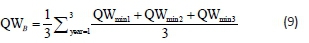
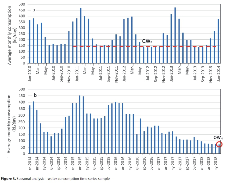
Consider Fig. 3, showing (a) a seasonal use pattern for a residential site and (b) the notably reduced summer use and changed seasonal pattern for the same site during the recent water restrictions (the data were lifted from one of the case study sites with residential homes, as reported on by Jacobs et al., 2020). The winter consumption for the baseline period QW_B is calculated as the average of the lowest three winter months in each year, and again taking the average of the three values over the three most recent baseline-years, as per Eq. 9. The three lowest values in any year are denoted QW_min1, QW_min2 and QW_min3:

The same procedure would not apply to the post-intervention period, because less than a full year of data would typically be available at the time of calculating the adjustment (the adjustment would be needed as soon as possible after introduction of water restrictions). After testing a few options, it was considered appropriate to select the single lowest value in the low-use season as the winter consumption QW_m for the post-intervention period during restrictions. The implication is that the adjustment could only be calculated after the first post-restriction low-use season had passed.

The reduction in winter consumption is likely ascribed to interventions by the WASCO, because the particular component of use would include all reduction of relatively constant leakage. The remaining portion of consumption is likely ascribed to external factors not introduced by the WASCO, meaning that two different factors are to be incorporated in this instance. Suggested values for factors β (pressure dependent seasonal component) and factor γ (pressure independent winter minimum component) are presented in Table 1.

Following similar logic as that explained to derive Eq. 6, the adjustment was found as follows, by assessing the saving by the service provider QS*:

The adjustment can now be calculated. The adjustment in Eq. 10 must equal the difference between the original QS calculation and the adjusted QS* as before. Substitute Eqs 2 and 10 into Eq. 5 to obtain the adjustment. Equation 11 is used to calculate the adjustment of the baseline (in kL/day) in cases where no MNF was available:

 

DISCUSSION

Calculation of a baseline adjustment as per the method presented in this paper, for Cases 1 to 3, relies on the availability of accurate monthly water consumption data, MNF, and/or pressure readings being available for the baseline site in question over a relatively long period. At some sites the required input data might not be available, but all parties may agree that an adjustment is needed to compensate for external influence on water saving. A fourth case, essentially the same as Case 1, would imply one in which the inputs would be crudely estimated. An informed decision regarding the level of leakage, based on limited measured data and records such as photos, maintenance records, pipe failure records, sewer baseflows downstream of the site, or even records of lush vegetation (in relation to the surrounding environment) in the proximity of suspected long-term pipe leaks. A record-based estimate of MNF (REM) could be obtained by assessing previously recorded, available information. If records pointing to real losses in the baseline period could be reviewed, MNF in the baseline period could be crudely estimated by means of REM, as per Fig. 4. The composition of Fig. 4 was based on knowledge of MNF and available records at the different study sample sites. Sites with a lack of data at this extreme level are unlikely to have had low MNF values in the baseline period, and a minimum value of 40% was considered reasonable in such cases. Some sites with MNF in excess of 90% were found in this case study, but 80% was considered a reasonable upper value in the absence of measured data. The post-intervention MNF could be determined by direct measurement in the post-baseline period (at the time when an adjustment has to be calculated). Given the estimated MNF in the baseline period, obtained with REM (Fig. 4), the adjustment could be calculated as per Eq. 6.

 

 

In the absence of measured data, and if the MNF could not be estimated by means of REM, then the adjustment could alternatively be calculated theoretically. A theoretical model would describe the water use in both periods as a function of numerous theoretical input parameters, all of which could be obtained by means of a desktop study and comprehensive site investigation. Numerous theoretical models are available for this purpose, but the results could be notably less accurate - with results influenced heavily by input data accuracy. Leakage could also be evaluated theoretically based on available drawings of the pipe network and estimates describing the number of connections, etc. In such cases assumptions of the ILI value, system pressure and leakage per service connection, would be required. Ideally a calibrated model should be developed for each site. With a calibrated model the expected water use could be predicted for pre- and post-intervention periods and savings could be modelled, then compared to actual savings on a month-by-month basis. However, a calibrated model would be data hungry, relatively complex and relies heavily on lengthy periods of accurately recorded data.

 

CONCLUSION

A baseline adjustment methodology for existing shared water savings contracts was devised, that could be implemented mid-contract, under conditions of limited data. The methodology was logically formulated by segregating water use and real losses. The procedure comprised three cases. Each case involved adjustment calculation with reduced accuracy, depending on the level of available data for the baseline site. In addition to monthly consumption data, the requirement for Case 1 was that MNF would be available in both pre- and post-intervention periods. Case 2 involved estimation of the MNF in one period based on knowledge of pressures, coupled with the pressure-leakage relationship and an assumed N1 value. The third case could be employed in the absence of MNF data, and involved adjustment calculation based exclusively on the monthly consumption. In all cases, a contribution factor is estimated to describe the relative contribution of the water services company's interventions to the resultant savings. The method is suitable for practical implementation in cases where data availability of a baseline site matches the input requirements.

 

ACKNOWLEDGEMENTS

The research results presented in this report emanate from a contract research project conducted by Stellenbosch University for the National Department of Public Works, South Africa. The methodology presented in this paper was the outcome of valuable contribution between the Stellenbosch University project team and all stakeholders at the NDPW, Re-Solve and the City of Cape Town. Minor inputs by postgraduate students Miss M Crouch and A Knox are also acknowledged. In particular, the authors would like to thank Mrs Kerry Fair (GLS) and Mr Lloyd Fisher-Jeffes (Aurecon, South Africa) for offering up their personal time to assist with various ad-hoc queries after hours.

 

REFERENCES

ALKASSEH JMA, ADLAN MN, ABUSTAN I and HANIF ABM (2015) Achieving an economic leakage level in Kinta Valley, Malaysia. Water Utility J. 11 31-47.         [ Links ]

ARBON N, THYER M, HATTON MACDONNALD D, BEVERLEY K and LAMBERT M (2014) Understanding and predicting household water us for Adelaide. Goyder Institute for Water Research Technical Report Series No. 14/15, Adelaide, South Australia.         [ Links ]

BEAL CD, STEWART R, HUANG T and REY E (2011) SEQ residential end use study. Aust. Water Assoc. J. 38 (1) 80-84.         [ Links ]

BLOKKER EJM, VREEBURG JHG and VAN DIJK JC (2010) Simulating residential water demand with a stochastic end-use model. J. Water Resour. Plan. Manage. 136 19-26. https://doi.org/10.1061/(ASCE)WR.1943-5452.0000002        [ Links ]

BUCHBERGER SG and NADIMPALLI G (2004) Leak estimation in water distribution systems by statistical analysis of flow readings. J. Water Resour. Plan. Manage. 130 321-329. https://doi.org/10.1061/(ASCE)0733-9496(2004)130:4(321)        [ Links ]

CHEUNG PB, GIROL GV, ABE N and PROPATO M (2010) Night flow analysis and modeling for leakage estimation in a water distribution system. Integrating water systems. Paper 89359. Proc. 10^th International Conference on Computing and Control for the Water Industry, CCWI 2009, 1-3 September 2009, University of Sheffield. 509-513.         [ Links ]

CORBETT CJ, DE CROIX GA and HA AY (2005) Optimal shared-savings contracts in supply chains: Linear contracts and double moral hazard. Eur. J. Oper. Res. 163 (3) 653-667. https://doi.org/10.1016/j.ejor.2004.01.021        [ Links ]

CSIR (2003) Guidelines for human settlement planning and design. Report compiled for the Department of Housing. Building and Construction Technology, Council for Scientific and Industrial Research, Pretoria.         [ Links ]

DI NARDO A, DI NATALE M, GISONNI C and IERVOLINO M (2015) A genetic algorithm for demand pattern and leakage estimation in a water distribution network. J. Water Suppl. Res. Technol. 64 (1) 35-46. https://doi.org/10.2166/aqua.2014.004        [ Links ]

DU PLESSIS JL and JACOBS HE (2015) Procedure to derive parameters for stochastic modelling of outdoor water use in residential estates. 13^th Computer Control for Water Industry Conference, CCWI 2015, 2-4 September 2015, Leicester, United Kingdom, Elsevier Ltd. Procedia Eng. 119 (2015) 803-812. https://doi.org/10.1016/j.proeng.2015.08.942        [ Links ]

GIUSTOLISI O, SAVIC D and KAPELAN Z (2008) Pressure driven demand and leakage simulation for water distribution networks. J. Hydraul. Eng. 134 (5) 626-635. https://doi.org/10.1061/(ASCE)0733-9429(2008)134:5(626)        [ Links ]

GOMES R, MARQUES AS and SOUSA J (2011) Estimation of the benefits yielded by pressure management in water distribution systems. Urban Water J. 8 (2) 65-77. https://doi.org/10.1080/1573062X.2010.542820        [ Links ]

GREYVENSTEIN B and VAN ZYL JE (2007) An experimental investigation into the pressure-leakage relationship of some failed water pipes. J. Water Suppl. Res. Technol. 56 (2) 117-124. https://doi.org/10.2166/aqua.2007.065        [ Links ]

JACOBS HE, DU PLESSIS JL, NEL N, GUGUSHE S and LEVIN S (2020) Baseline adjustment in a shared water saving contract during severe water restrictions - a case study in the Western Cape, South Africa. Water SA 46 (1) xxxx.         [ Links ]

JACOBS HE, SCHEEPERS HM and SINSKE SA (2013) Effect of land area on average annual suburban water demand. Water SA 39 (5) 687-694. http://dx.doi.org/10.4314/wsa.v39i5.13        [ Links ]

JACOBS HE, GEUSTYN LC, LOUBSER BF and VAN DER MERWE B (2004). Estimating residential water demand in Southern Africa. J. S. Afr. Inst. Civ. Eng. 46 (4) 2-13.         [ Links ]

JACOBS HE and HAARHOFF J (2004) Structure and data requirements of an end-use model or residential water demand and return flow. Water SA 30 (3) 293-304. https://doi.org/10.4314/wsa.v30i3.5077        [ Links ]

LAMBERT AO (2002) International report: Water losses management and techniques. Water Sci. Technol. Water Suppl. 2 (4) 1-20. https://doi.org/10.2166/ws.2002.0115        [ Links ]

LAMBERT AO (1994). Accounting for Losses: The bursts and background concept. Water Environ. J. 8 (2) 205-214. https://doi.org/10.1111/j.1747-6593.1994.tb00913.x        [ Links ]

MAY JH (1994) Pressure dependent leakage. World Water and Environmental Engineering, October 1994. Technical Report. Water Environment Federation, Washington, DC.         [ Links ]

MAYER PW, DEOREO WB, TOWLER E AND LEWIS DM (2003) Residential indoor water conservation study: Evaluation of high efficiency indoor plumping fixture retrofits in single-family homes in the East Bay Municipal Utility District Service Area. Aquacraft, Inc., Boulder, CO.         [ Links ]

MCKENZIE R (2001) Development of a pragmatic approach to evaluate the potential savings from pressure management in potable was distributions in South Africa: PRESMAC. WRC Report No. TT 152/01. Water Research Commission, Pretoria. ISBN No. 1 86845 722 2        [ Links ]

MCKENZIE RS (2002) Khayelitsha: Leakage reduction through advanced pressure control. J. Inst. Munic. Eng. S. Afr. 27 (8) 43-47.         [ Links ]

MCKENZIE RS, LAMBERT AO, KOCK JE and MTSHWENI W (2002) Development of a simple and pragmatic approach to benchmark real losses in potable was distribution systems in South Africa': BENCHLEAK. WRC Report No. TT 159/01. Water Research Commission, Pretoria. ISBN No. 1 86845 773 7        [ Links ]

MCKENZIE RS, MOSTERT H and WEGELIN W (2003) Leakage reduction through pressure management in Khayelitsha, Western Cape: South Africa. Paper presented at the Australian Water Association Annual Conference, 7-10 April 2003, Perth.         [ Links ]

MEYER N, JACOBS HE, WESTMAN T and MCKENZIE RS (2018) The effect of controlled pressure adjustment in an urban water distribution system on household demand. J. Water Suppl. Res. Technol. 67 (3) 218-226. https://doi.org/10.2166/aqua.2018.139        [ Links ]

MUTIKANGA HE, SHARMA SK and VAIRAVAMOORTHY K (2013) Methods and tools for managing losses in water distribution systems. J. Water Resour. Plann. Manage. 139 (2) 166-174. https://doi.org/10.1061/(ASCE)WR.1943-5452.0000245        [ Links ]

NSANZUBUHORO R and VAN ZYL JE (2018) Characterising leakage in a real transmission main by means of a pipe condition assessment equipment. 1^st International WDSA-CCWI 2018 Joint Conference, 23-25 July 2018, Kingston, Ontario, Canada.         [ Links ]

ROSSI F, VELAZQUES D, MONEDERO I and BISCARRI F (2014) Artificial neural networks and physical modeling for determination of baseline consumption of CHP plants. Expert Syst. Appl. 41 (10) 4658-4669. https://doi.org/10.1016/j.eswa.2014.02.001        [ Links ]

SCHEEPERS HM and JACOBS HE (2014) Simulating residential indoor water demand by means of a probability based end-use model. J. Water Suppl. Res. Technol. 66 (3) 476-488. https://doi.org/10.2166/aqua.2014.100        [ Links ]

SEAGO C, BHAGWAN J and MCKENZIE RS (2004) Benchmarking leakage from water reticulation systems in South Africa. Water SA 30 (5) 25-32. https://doi.org/10.4314/wsa.v30i5.5162        [ Links ]

SCHWALLER J and VAN ZYL JE (2014) Modeling the pressure-leakage response of water distribution systems based on individual leak behavior. J. Hydraul. Eng. 04014089 1-8. https://doi.org/10.1061/(ASCE)HY.1943-7900.0000984        [ Links ]

STRIJDOM L, SPEIGHT V and JACOBS HE (2017) Theoretical evaluation of sub-standard water network pressures. J. Water Sanit. Hyg. Dev. 7 (4) 557-567. https://doi.org/10.2166/washdev.2017.227        [ Links ]

USDE (United States Department of Energy) (2001) International Performance Measurement & Verification Protocol. Concepts and Options for Determining Energy and Water Savings. Volume I. International Performance Measurement & Verification Protocol Committee, January 2001. DOE/GO-102001-1187.         [ Links ]

VAN ZYL JE and MALDE R (2017) Evaluating the pressure-leakage behaviour of leaks in water pipes. J. Water Suppl. Res. Technol. 66 (5) 287-299. https://doi.org/10.2166/aqua.2017.136        [ Links ]

WEGELIN W and MCKENZIE RS (2005) Sebokeng Evaton pressure leakage reduction: Public private partnership. Proceedings from the International Water Association Specialist Conference: Leakage 2005, 12-14 September 2005, Halifax, Nova Scotia, Canada. 382-391.         [ Links ]

 

 

Correspondence:
HE Jacobs
hejacobs@sun.ac.za

Received: 23 October 2018
Accepted: 15 November 2019