KOLDING J and VAN ZWITTEN PAM (2012) Relative lake level fluctuations and their influence on productivity and resilience in tropical lakes and reservoirs. Fish. Res. (115-116) 99-109. https://doi.org/10.1016/j.fishres.2011.11.008        [ Links ]

IRVINE K, ETIEGNI CA and WEYL OLF (2018) Prognosis for long term sustainable fisheries in the African Great Lakes. Fish. Manage. Ecol. 00 1-13. https://doi.org/10.1111/fme.12282        [ Links ]

LINK JS, THÉBAUD O, SMITH DC, SMITH ADM, SCHMIDT J, RICE J, POOS JJ, PITA C, LIPTON D, KRAAN M and co-authors (2017) Keeping humans in the ecosystem. ICES J. Mar. Sci. 74 1947-1956. https://doi.org/10.1093/icesjms/fsx130        [ Links ]

MAGADZA CHD (2003) Lake Chivero: A management case study. Lakes Reserv. Res. Manage. 8 69-81. https://doi.org/10.1046/j.1320-5331.2003.00214.x        [ Links ]

MARSHALL BE (2011) Fishes of Zimbabwe and their Biology. Smithiana Monograph 3. The Southern African Institute for Aquatic Biodiversity, Grahamstown.         [ Links ]

NAGENDRA H and OSTROM E (2014) Applying the social-ecological system framework to the diagnosis of urban lake commons in Bangalore, India. Ecol. Soc. 19 (2) 67-72. https://doi.org/10.5751/ES-06582-190267        [ Links ]

NELSON R, HOWDEN SM and STAFFORD SMITH M (2008) Using adaptive governance to rethink the way science supports Australian drought policy. Environ. Sci. Polic. 11 588-601. https://doi.org/10.1016/j.envsci.2008.06.005        [ Links ]

NHAPI I and GIJZEN HJ (2004) Wastewater management in Zimbabwe in the context of sustainability, Water Polic. J. 6 (6) 115-121. https://doi.org/10.2166/wp.2004.0033        [ Links ]

NHIWATIWA T, BARSON M, HARRISON AP, UTETE B and COOPER RG (2011) Metal concentrations in sharptooth catfish (Clarias gariepinus, Burchell 1822), sediments and water in peri-urban rivers in Zimbabwe. Afr. J. Aquat. Sci. 3 243-252. https://doi.org/10.2989/16085914.2011.636906        [ Links ]

NYARUMBU TO and MAGADZA CHD (2016) Using the Planning and Management Models of Lakes and Reservoirs (PAMOLARE) as a tool for planning the rehabilitation of Lake Chivero, Zimbabwe. Environ. Nano. Monit. Manage. 5 1-12. https://doi.org/10.1016/j.enmm.2015.10.002        [ Links ]

STEPHENSON RL, PAUL S, WIBER M, ANGEL E, BENSON AJ, CHARLES A, CHOUINARD O, CLEMENS M, EDWARDS D, FOLEY P and co-authors (2018) Evaluating and implementing social-ecological systems: A comprehensive approach to sustainable fisheries. Fish Fish. 19 (5) 853-873. https://doi.org/10.1111/faf.12296        [ Links ]

TAYLOR WW, LEONARD NJ, KRATZER JF, GODDARD C and STEWART P (2007) Globalization: implications for fish, fisheries and their management. In: Taylor WW, Schechter MG and Wolfson LG (eds) Globalization: Effects on Fisheries Resources. Cambridge University Press, Cambridge, UK. 21-46 pp. https://doi.org/10.1017/CBO9780511542183.005        [ Links ]

TENDAUPENYU P (2012) Nutrient limitation of phytoplankton in five impoundments on the Manyame River, Zimbabwe. Water SA 38 (1) 97-104. https://doi.org/10.4314/wsa.v38i1.12        [ Links ]

TWEDDLE D, COWX IG, PEEL R and WEYL OLF (2015) Challenges in fisheries management in the Zambezi, one of the great rivers of Africa. Fish. Manage. Ecol. 22 99-111. https://doi.org/10.1111/fme.12107        [ Links ]

UTETE, B, PHIRI C, MLAMBO SS, MUBOKO N and FREGENE BT (2018) Fish catches, and the influence of climatic and non-climatic factors in Lakes Chivero and Manyame, Zimbabwe. Cogent Food Agric. 4 (1) https://doi.org/10.1080/23311932.2018.1435018        [ Links ]

VÖRÖSMARTY CJ, MCINTYRE PB, GESSNER MO, DUDGEON D, PRUSEVICH A, GREEN P and GLIDDEN S (2010) Global threats to human water security and river biodiversity. Nature 467 (7315) 555-561. https://doi.org/10.1038/nature09440        [ Links ]

WELCOMME RL, COWX IG, COATES D, BÉNÉ C, FUNGE-SMITH S, HALLS A and LORENZEN K (2010) Inland capture fisheries. Phil. Trans. of the Royal Soc. of Biol. 365 2881-2896. https://doi.org/10.1098/rstb.2010.0168        [ Links ]

WEPENER W, VAN VUREN JHJ and DU PREEZ HH (2001) Uptake and Distribution of a copper, iron and zinc mixture in gill, live rand plasma of a freshwater teleost, Tilapia sparmanii. Water SA 27 (1) 99-108. https://doi.org/10.4314/wsa.v27i1.5016        [ Links ]

WICHELNS D (2017) The water-energy-food nexus: Is the increasing attention warranted, from either a research or policy perspective? Environ. Sci. & Pol. 69 113-123. https://doi.org/10.1016/j.envsci.2016.12.018        [ Links ]

WorldFish Center (2009) Fish and aquaculture in a changing climate. Proceedings from the UNFCCC COP-15, December 2009, Copenhagen.         [ Links ]

 

 

Received 9 August 2018
Accepted in revised form 26 September 2019

 

 

* Corresponding author, email: mkaiyo@gmail.com

^rND^sADELEKAN^nI^rND^sFREGENE^nT^rND^sALLISON^nEH^rND^sHOREMANS^nB^rND^sALLISON^nE^rND^sELLIS^nF^rND^sALLISON^nEH^rND^sPERRY^nAL^rND^sBADJECK^nMC^rND^sADGER^nWN^rND^sBROWN^nK^rND^sCONWAY^nD^rND^sHALLS^nAS^rND^sPILLING^nGM^rND^sREYNOLDS^nJD^rND^sANDREW^nNL^rND^sDULVY^nN^rND^sANDERSON^nJL^rND^sANDERSON^nCM^rND^sCHU^nJ^rND^sMERIDETH^nJ^rND^sASCHE^nF^rND^sSYLVIA^nG^rND^sVALDERRAMA^nD^rND^sBARTLEY^nDM^rND^sde GRAAF^nGJ^rND^sVALBO-JØRGENSEN^nJ^rND^sMARMULLA^nG^rND^sBÉNÉ^nC^rND^sBÉNÉ^nC^rND^sNEILAND^nAE^rND^sJOLLEY^nT^rND^sOVIE^nS^rND^sSULE^nO^rND^sLADU^nB^rND^sMINDJIMBA^nK^rND^sBELAL^nE^rND^sTIOTSOP^nF^rND^sBABA^nM^rND^sDARA^nL^rND^sZAKARA^nA^rND^sQUENSIERE^nJ^rND^sBÉNÉ^nC^rND^sBÉNÉ^nC^rND^sSTEEL^nE^rND^sKAMBALA LUADIA^nB^rND^sGORDON^nA^rND^sBOYD^nH^rND^sCHARLES^nA^rND^sBRANDER^nK^rND^sCHU^nJ^rND^sGARLOCK^nT^rND^sASCHE^nF^rND^sANDERSON^nJL^rND^sCOOKE^nSJ^rND^sPAUKERT^nC^rND^sHOGAN^nZ^rND^sCOOKE^nSJ^rND^sLAPOINTE^nNWR^rND^sMARTINS^nEG^rND^sTHIEM^nJD^rND^sRABY^nGD^rND^sTAYLOR^nMK^rND^sBEARD^nTDJR^rND^sCOWX^nIG^rND^sGARCIA^nSM^rND^sROSENBERG^nAA^rND^sHOWELLS^nMS^rND^sHERMANN^nM^rND^sWELSCH^nM^rND^sBAZILIAN^nR^rND^sSEGERSTRÖM^nR^rND^sALFSTAD^nD^rND^sGIELEN^nH^rND^sROGNER^nG^rND^sFISCHER^nH^rND^sVAN VELTHUIZEN^nD^rND^sKOLDING^nJ^rND^sVAN ZWITTEN^nPAM^rND^sIRVINE^nK^rND^sETIEGNI^nCA^rND^sWEYL^nOLF^rND^sLINK^nJS^rND^sTHÉBAUD^nO^rND^sSMITH^nDC^rND^sSMITH^nADM^rND^sSCHMIDT^nJ^rND^sRICE^nJ^rND^sPOOS^nJJ^rND^sPITA^nC^rND^sLIPTON^nD^rND^sKRAAN^nM^rND^sMAGADZA^nCHD^rND^sNAGENDRA^nH^rND^sOSTROM^nE^rND^sNELSON^nR^rND^sHOWDEN^nSM^rND^sSTAFFORD SMITH^nM^rND^sNHAPI^nI^rND^sGIJZEN^nHJ^rND^sNHIWATIWA^nT^rND^sBARSON^nM^rND^sHARRISON^nAP^rND^sUTETE^nB^rND^sCOOPER^nRG^rND^sNYARUMBU^nTO^rND^sMAGADZA^nCHD^rND^sSTEPHENSON^nRL^rND^sPAUL^nS^rND^sWIBER^nM^rND^sANGEL^nE^rND^sBENSON^nAJ^rND^sCHARLES^nA^rND^sCHOUINARD^nO^rND^sCLEMENS^nM^rND^sEDWARDS^nD^rND^sFOLEY^nP^rND^sTAYLOR^nWW^rND^sLEONARD^nNJ^rND^sKRATZER^nJF^rND^sGODDARD^nC^rND^sSTEWART^nP^rND^sTENDAUPENYU^nP^rND^sTWEDDLE^nD^rND^sCOWX^nIG^rND^sPEEL^nR^rND^sWEYL^nOLF^rND^sUTETE^nB^rND^sPHIRI^nC^rND^sMLAMBO^nSS^rND^sMUBOKO^nN^rND^sFREGENE^nBT^rND^sVÖRÖSMARTY^nCJ^rND^sMCINTYRE^nPB^rND^sGESSNER^nMO^rND^sDUDGEON^nD^rND^sPRUSEVICH^nA^rND^sGREEN^nP^rND^sGLIDDEN^nS^rND^sWELCOMME^nRL^rND^sCOWX^nIG^rND^sCOATES^nD^rND^sBÉNÉ^nC^rND^sFUNGE-SMITH^nS^rND^sHALLS^nA^rND^sLORENZEN^nK^rND^sWEPENER^nW^rND^sVAN VUREN^nJHJ^rND^sDU PREEZ^nHH^rND^sWICHELNS^nD^rND^1A01^nDavid^sLe Maitre^rND^nAndré^sGörgens^rND^nGerald^sHoward^rND^1A02^nNick^sWalker^rND^1A01^nDavid^sLe Maitre^rND^nAndré^sGörgens^rND^nGerald^sHoward^rND^1A02^nNick^sWalker^rND^1A01^nDavid^sLe Maitre^rND^nAndré^sGörgens^rND^nGerald^sHoward^rND^1A02^nNick^sWalker

RESEARCH PAPERS

 

Impacts of alien plant invasions on water resources and yields from the Western Cape Water Supply System (WCWSS)

 

 

David Le Maitre^{I, II, *}; André Görgens^III; Gerald Howard^III; Nick Walker^{III, IV, V}

^INatural Resources and the Environment, CSIR, Stellenbosch
^IICentre for Invasion Biology, Department of Botany and Zoology, Stellenbosch University, South Africa
^IIIAurecon South Africa (Pty) Ltd, Cape Town, South Africa
^IVERM, One Castle Park, Tower Hill, Bristol, United Kingdom
^VInstitute of Water Studies, University of the Western Cape, Bellville, South Africa

 

 

---

ABSTRACT

A key motivation for managing invasive alien plant (IAP) species is their impacts on streamflows, which, for the wetter half of South Africa, are about 970 m³∙ha⁻¹∙a⁻¹ or 1 444 mill. m³∙a⁻¹ (2.9% of naturalised mean annual runoff), comparable to forest plantations. However, the implications of these reductions for the reliability of yields from large water supply systems are less well known. The impacts on yields from the WCWSS were modelled under three invasion scenarios: 'Baseline' invasions; increased invasions by 2045 under 'No management'; and under 'Effective control' (i.e. minimal invasions). Monthly streamflow reductions (SFRs) by invasions were simulated using the Pitman rainfall−runoff catchment model, with taxon-specific mean annual and low-flow SFR factors for dryland (upland) invasions and crop factors for riparian invasions. These streamflow reduction sequences were input into the WCWSS yield model and the model was run in stochastic mode for the three scenarios. The 98% assured total system yields were predicted to be ±580 million m³∙a⁻¹ under 'Effective control', compared with ±542 million m³∙a⁻¹ under 'Baseline' invasions and ±450 mill. m³∙a⁻¹ in 45 years' time with 'No management'. The 'Baseline' invasions already reduce the yield by 38 mill. m³∙a⁻¹ (two thirds of the capacity of the Wemmershoek Dam) and, in 45 years' time with no clearing, the reductions would increase to 130 mill. m³∙a⁻¹ (capacity of the Berg River Dam). Therefore IAP-related SFRs can have significant impacts on the yields of large, complex water supply systems. A key reason for this substantial impact on yields is that all the catchments in the WCWSS are invaded, and the invasions are increasing. Invasions also will cost more to clear in the future. So, the best option for all the water-users in the WCWSS is a combined effort to clear the catchments and protect their least expensive source of water.

Keywords: invasive alien plants, hydrological impacts; streamflow reduction, system yield

---

 

 

INTRODUCTION

Concerns about the impacts of alien plant invasions on streamflows were a key factor in the establishment of the Working for Water programme in October 1995 and in sustaining the programme since then (Le Maitre et al., 1996; Le Maitre et al., 2000; Van Wilgen et al., 1998). The streamflow reduction models used to estimate the flow reductions were based on long-term studies of the impacts of plantations on streamflows in catchments spread across South Africa compared with natural vegetation, particularly fynbos (Van Wyk, 1987; Van Lill et al., 1980; Bosch et al., 1980; Bosch and Von Gadow, 1990). The invasions often involved the same or ecologically similar tree species as those in the plantation studies, strengthening the argument that the reductions caused by invasions could match those observed in plantation studies (Le Maitre et al., 1996; Le Maitre, 2004). Ongoing research into water use by individual plants and stands of invasive species (Everson et al., 2014; Dzikiti et al., 2013; Meijninger and Jarmain, 2014; Dye and Jarmain, 2004) has confirmed the original findings, and shown that invasions can have substantial impacts on streamflows (see review by Le Maitre et al., 2015).

There is still an ongoing debate, though, about the impacts of flow reductions on the yields from large water supply schemes (WSS). Yet, there is every indication that the reductions in flows will result in reductions in yields, for a given level of assurance of supply, even when the storage dams in the WSS are large relative to the mean annual runoff (Le Maitre and Görgens, 2001; Cullis et al., 2007). These findings have not convinced some who argue that it is more cost-effective to build additional storage or transfer schemes to supply additional water than to clear invasions. While WSS infrastructure is necessary, and WSS capacity does need augmenting to meet increases in demand (Muller et al., 2015), investments in additional infrastructure can be unwise if the reductions more than offset the gains provided by the infrastructure, or if alternative water resources are considerably more expensive to develop or inherently more costly, such as desalinisation. One way of comparing such investments is the unit reference value which calculates the net present value of the costs of different investments (e.g. in infrastructure) over the projected life-span of the infrastructure, and relates it to the volume of water yielded to derive a cost per m³ of water (Van Niekerk and Du Plessis, 2013).

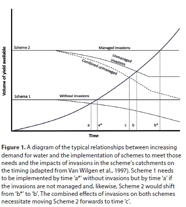
Although the unit reference value (URV) is a useful way of comparing investments in water supply infrastructure in relation to their yields, the way it is used in practice treats the decreased yields from the one option as being replaceable with yields from other options (Fig. 1). Van Wilgen et al. (1997) presented a simple model to illustrate how the impacts of unmanaged invasions on water yields would affect water yields over time. This model was very similar to the one in Fig. 1 and showed how the timing of the development of two water supply schemes was affected by invasions. Van Wilgen et al. (1997) also showed that differing initial stages of invasion and differing proportions of non-invadable areas would affect the outcomes, illustrated here by the different rates of reduction of flows from the catchments in the two schemes and stabilisation of the reductions from Scheme 2. With invasions, Scheme 1 would have to be operational by year 'a' to meet the rising demand but with clearing could be postponed to year 'a*'. Likewise Scheme 2 could be delayed from 'b' to 'b*'. However, their model failed to take into account the fact that without clearing, the ongoing decline in the yields from the original sources (Fig. 1), combined with the declining yield from Scheme 2, would require Scheme 2 to be operational by time 'c' and would also bring forward any future schemes. The WCWSS borders on the coast so desalinisation could be an option for meeting rising demand but, if there really were no more land-based options for increasing yields, the only choice would be to clear the invasions. However, by time 'c' arrives, the costs of clearing the invasions would also have increased significantly, a factor which also needs to be taken into consideration. The standard discounting model used in estimating the net present values for the URV would discount those future costs, essentially assuming that some innovative technologies would drastically lower the clearing costs by time 'c', but this is highly unlikely to be the case. If anything, the costs are likely to be significantly higher because the currently relatively lightly invaded, rugged mountain areas which comprise much of the WCWSS's catchments would have become more densely invaded. Clearing these areas is very expensive as it requires fit, able and skilled people, and expensive safety equipment, as well as the costs incurred in supporting workers camping-out for a week at a time where daily access is not efficient. The rate at which invaders are cleared also is low because the people have to use ropes for safety and moving between plants and safely securing themselves is very time consuming. In other words, if there is a finite yield of water from the current WSS, and this will be significantly reduced by allowing alien plants to invade the catchments, then clearing now would be the best option for securing overall yields in the long-term, even if the unit reference values are higher. Thus, clearing invasions now represents a much wiser investment of resources than deferring clearing. If this is so, then it provides a sound rationale for ensuring that a portion of the revenue realised from supplying water to users is dedicated to clearing the catchment and ensuring that invasions are cleared as rapidly as possible to as low a density as possible, and the catchment maintained in that state.

 

 

This paper focuses on the potential impact of invasions on the water yields of the Western Cape Water Supply System (WCWSS) which supplies water to the City of Cape Town as well as some adjacent local authorities and irrigation schemes Van Wilgen et al. (1997) found that clearing of invasive alien plants in the catchment of the Berg River Dam, then known as the Skuifraam scheme, would deliver water at a unit reference value of 0.57 ZAR∙m⁻³ compared with 0.59 ZAR∙m⁻³ without clearing over a 45-year period. The modelling used a discount rate of 8% and increases in invasion densities were driven by fires every 15 years, this being the desired fire return period in fynbos. Clearing of invasions in the Theewaterskloof Dam catchment, which was more heavily invaded than the Berg River Dam catchment, would be much more cost effective, with a unit reference value of 0.08 ZAR∙m⁻³ compared with 0.59 ZAR∙m⁻³ without clearing. This study, among others, motivated the then Department of Water Affairs to ensure that provision was made for alien plant clearing in the budget for the construction of the Berg River Dam (Geland et al., 2008). The funding provided for the clearing of pine plantations and invasions on the lower slopes within the catchment of the dam itself by the construction company. In addition, the Working for Water Programme contributed funding for the clearing of the rest of the catchment and areas situated below the dam wall.

Our study area included the entire WCWSS and used updates of the streamflow reduction models (Le Maitre et al., 2013), which allowed for distinctions between plant species and between riparian and non-riparian invasions, to estimate the impacts on yields.

 

STUDY AREA

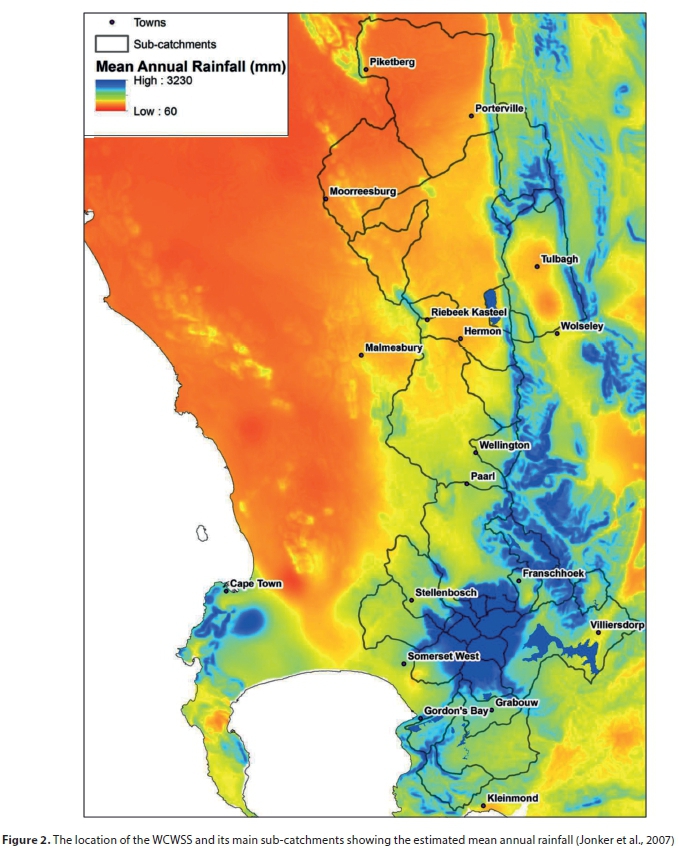
The study is located in a set of catchments to the west and north of the Cape Metropole (CM) in the Western Cape Province (https://www.dwa.gov.za/Projects/RS_WC_WSS/) (DWS, 2014) (Fig. 2). The WCWSS includes catchments located in the headwaters of different river systems in the Boland mountains which receive the highest rainfall in South Africa (Fig. 2). The WCWSS has a complex set of inter-basin water transfer systems which allow water to be provided to different parts of the Cape Metropole (CM), to neighbouring towns and to various irrigation schemes. The main transfer is from the Theewaterskloof Dam in the Riviersonderend catchment (H6) to the CM via a tunnel system that links it to the Berg (G1) and Eerste River (G2) catchments. Water is also transferred to the CM from the Steenbras (G4) and Palmiet (G4) catchments and from the Berg River and Wemmershoek Dams in the Berg River catchment (G1). The Voëlvlei Dam transfers water from the Klein Berg and 24 Rivers catchments to parts of the CM and towns in the northern part of the Berg River catchment. The WCWSS can yield about 580 mill. m³∙a⁻¹ at a 98% level of supply assurance (i.e. a 1 in 50 year probability of not being able to supply this volume of water). Further optimisation of the storage in the WCWSS could increase the yield to 596 mill. m³∙a⁻¹, at the same level of assurance.

 

 

 

METHODS

Alien plant invasion data

Datasets on alien plant invasions were obtained from a range of sources, updated and combined to produce a dataset for the whole area covered by the catchments in the WCWSS. The spatial datasets were as follows:

1.Invasion mapping done for an assessment of water availability in the Berg Water Management Area (WMA 19) carried out by Aurecon (supplied by Cheryl Beuster of Aurecon) and known as the Berg WAAS (DWAF, 2010). This dataset was edited to correct species attribute data as verified in the field, mainly where pines were listed when the actual dominants were Populus species, Eucalyptus species and Acacia species. The plantation dataset from this same study was checked to confirm whether or not these areas were plantations and not unmanaged invasions.

2.Data from CapeNature based on mapping of the invasions in the management compartments in the nature reserves that overlapped with the study catchments (supplied by Therese Forsyth). This mapping was done in 2010/11.

3.In the Upper Berg (G10A) information was taken from mapping done by the CSIR for the Working for Water programme in 2000. This was cross-checked with data on the pre-treatment state of areas cleared under Working for Water contracts. Data extracted from the Working for Water Information Management System were used to refine the information on invasions in both the Franschhoek River and Berg River catchments.

4.Data for invasions in the lower catchment from mapping done for local municipalities in the early 2000s for the CAPE Fine-scale Conservation Planning Studies, and the West Coast invasion mapping done for the CAPE project in 1999. These datasets were cross-checked and compared with Google Earth images to reflect the state of invasions in the late-2000s to bring them in line with the Berg WAAS.

5.Additional polygon data were mapped in Google Earth from images dating from the early to middle 2000s to avoid including more recent clearing operations.

The species data for the combined set was edited to ensure that the species names and density values were consistent. Each of the invaded units (polygons) was identified as being riparian or non-riparian, or one where groundwater could be accessed by plant root systems. This information was required for the estimation of the hydrological impacts as an indication of relative water availability (Le Maitre et al., 1996; Le Maitre et al., 1999, 2013). Where necessary, invaded polygons were sub-divided to define the riparian sections more accurately. The datasets were then combined with data on the sub-catchment boundaries of the WCWSS to provide information on the extent and state of invasions in each of the sub-catchments in dryland, riparian and groundwater settings.

The existing invasions were then projected forwards for 45 years using a sigmoidal curve for the spread as has been found in many studies of invasions (Le Maitre et al., 2002; Hengeveld, 1989; Birks, 1989), a spread rate of 10% per year (Van Wilgen and Le Maitre, 2013) and a densification rate of 1% per year. The use of this model results in slow initial invasion followed by a rapid increase which then slows as the invadable land becomes fully occupied. The National Land Cover 2000 dataset (Van den Berg et al., 2008) was used to extract the remaining natural (i.e. invadable) areas in each sub-catchment by excluding all the transformed land classes (e.g. cultivated, forest plantation, urbanised). The river lines from 1:50 000 topographic map series were buffered to create a layer which defined the riparian zones. Areas mapped in the land-types (LTSS, 1972-2002) as having deep sandy soils were used to define areas where groundwater would be accessible to plant root systems (Le Maitre et al., 2013). This information was used to divide the potentially invadable areas into drylands, riparian and groundwater access for the spread modelling. The projection of the invasions was then done for each sub-catchment in a spreadsheet.

Invasion scenarios

The approach taken in this study is the same as was used in previous studies of the effects of 'No management' on invasions (Le Maitre et al., 2002; Van Wilgen et al., 1997). We selected the year 2000 as the base year for the simulations and projected invasions forwards to 2045 because 45 years generally is used as the life-span of the infrastructure in assurance of supply studies like this one. The 2000 invasion data were used to establish the 'Baseline' scenario, with the projected invasions in the year 2045 providing the 'No management' scenario and removal of all invasions the 'Effective management' scenario.

Estimating streamflow reductions

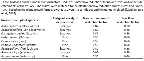
One of the criticisms levelled at the original flow reduction model developed for invasions (Le Maitre et al., 1996) was that the reductions were estimated as the equivalent depth (i.e. mm), which can result in overestimations. This was addressed by revising the approach to estimate proportional reductions (Dzvukamanja et al., 2005; Le Maitre et al., 2013), like those formerly used to estimate reductions after commercial afforestation (Scott and Smith, 1997). This meant that reductions caused by dryland invasions could be estimated by matching the plant growth and growth form characteristics to those used in the plantation streamflow reduction models (Table 1).

 

 

Whilst this approach can be used for dryland invasions, it is likely to underestimate water-use in riparian invasions or where groundwater is accessible (Le Maitre et al., 2015). In riparian and groundwater settings evaporation from vegetation is driven mainly by the available energy and can exceed the annual rainfall if sufficient water is available (Dye and Jarmain, 2004; Everson et al., 2014; Le Maitre et al., 2015), providing the plants' hydraulic conductivity is high enough and they do not regulate their transpiration by closing stomata when internal moisture stress or vapour pressure deficits are high (Manzoni et al., 2013; Calder, 1991; Whitehead and Beadle, 2004; Jarvis and McNaughton, 1986).

The evaporation from riparian or groundwater-linked stands of invading plants can be estimated using micrometeorological techniques or remote sensing. The CSIR obtained high-resolution, remote-sensing estimates of evaporation (Et) for two sample areas in the upper part of the Berg River catchment from the eLEAF Competence Centre in The Netherlands - these being Franschhoek to Klapmuts, and the Berg River floodplain for 5 km upstream of Hermon (Le Maitre et al., 2016). The Et was estimated using the proprietary Surface Energy Balance (SEBAL) model (Bastiaanssen et al., 1998) as part of a study of irrigation water-use in the wine and deciduous fruit growing areas of the Western Cape, known as Fruitlook (http://fruitlook.co.za/). eLEAF provided estimates of the weekly evaporation from 2 October 2013 to 29 April 2014 and for individual cloud-free days which coincided with satellite passes from May to September 2014. The data are at a resolution of 20 x 20 m which is suitable for estimating annual evaporation from fairly narrow strips of riparian vegetation.

Riparian invasions which overlapped the two sample areas were selected from the mapped data and screened for those dominated by particular species and having natural riparian vegetation in good condition. Invaded areas situated on steep southerly aspects were avoided as they are subject to topographic shading effects which are a problem for energy-balance-based methods like SEBAL. Evaporation data for each of the sample periods was extracted and used to calculate the monthly and annual evaporation. The weekly data were simply summed as they provided a continuous record. The single day data for the winter period were multiplied up by the number of days in the month to calculate the corresponding monthly totals (Table 2). This approach could overestimate the monthly total as there are many cloudy days, but a comparison with measured evaporation for the same days and for the month at a site near Hermon (Dzikiti et al., 2016) suggested that the overestimate for those months was not significant. However, the SEBAL data were found to overestimate evaporation by about 20% compared with ground-based measurements. Unfortunately it is difficult to correct for this for all the invaded areas without more ground-truthing at other sites, especially in montane environments. However, what really matters for the modelling is the difference in the evaporation from invaded riparian and natural riparian areas which is less influenced by this systematic error. The values that were obtained are in line with those from other studies for similar species, for example Acacia mearnsii (Dye and Jarmain, 2004), especially given that subsequent work has found much greater interception losses in stands of this species (Everson et al., 2014).

Modelling streamflow reductions

Flow reductions for invaded upland areas were estimated from taxon-specific streamflow reduction factors (Table 1). In areas where groundwater was likely to be accessible to invading plants (e.g. deep sandy soils), the upland flow reduction factors were increased by 20% to allow for the greater water availability (Van Wilgen et al., 2008). Riparian IAPs have relatively direct access to water, both in the riparian soil and flowing past from upstream. The impacts of riparian invasions were estimated using data on the actual evapotranspiration for the different taxa (Table 2). A spread-sheet was set up for each sub-catchment to generate a time series of riparian streamflow reduction as follows: (i) Multiply the invaded riparian area in the sub-catchment for particular taxa by the 12 relevant mean actual monthly evapotranspiration values (Table 2); (ii) determine the 12 incremental mean monthly evapotranspiration values from each taxon after accounting for the mean monthly evapotranspiration from 'natural' riparian vegetation (indigenous montane); and (iii) for each taxon generate a time series of dynamically-varying incremental monthly evapotranspiration values by inverse weightings derived from the sub-catchment monthly rainfall sequence, standardised to reproduce the 12 mean incremental values derived in step (ii) above. This inverse procedure ensured that, during any high-rainfall month, the incremental evapotranspiration was less than the equivalent value in Table 2 for that month and vice versa, while preserving the 12 long-term means. The magnitude of the riparian streamflow reduction in several catchments was so small that it became necessary to add the riparian SFRs for several catchments together. A total of seven riparian streamflow reduction locations were used in the yield model to assess the flow reductions evenly throughout the WCWSS.

Configuring and running the Pitman rainfall−runoff and WRYM system yield models

The full set of configurations of the Pitman (WRSM2000) rainfall−runoff catchment model for all the sub-catchments used in the Berg WAAS (DWAF, 2010) was de-archived and checked for functionality. The invaded area coverages were intersected with the individual sub-catchment boundaries used in the WCWSS WRYM system yield model (hereafter WRYM) and the individual IAP taxon areas, and their densities, quantified on a sub-catchment basis. These data were then used as input to the Pitman catchment model for the generation of monthly SFR sequences per sub-catchment for each of the three scenarios. The information on the invasions and streamflow reductions was included in the Pitman model configuration files and the model was then run to generate sequences of monthly streamflows for all sub-catchments for the three invasion scenarios. These streamflows were used to populate the latest configuration of the WRYM (DWS, 2014).

The WRYM model configuration was modified to accommodate a large number of additional SFR 'demand' nodes necessitated by the updated IAP mapping and the scenarios. The Pitman-generated SFR sequences were input into the system model as 'demand' files at each of the aforementioned nodes. The historical time period covered by the WRYM simulations is 77 hydrological years (1928/29-2005/06). The system model was subsequently run in stochastic mode to determine yield-assurance relationships for the three scenarios. For this purpose, and for each scenario, 201 different sets of equally likely stochastic natural streamflow sequences, based on the historical sequence, were generated for all the streamflow input nodes.

 

RESULTS

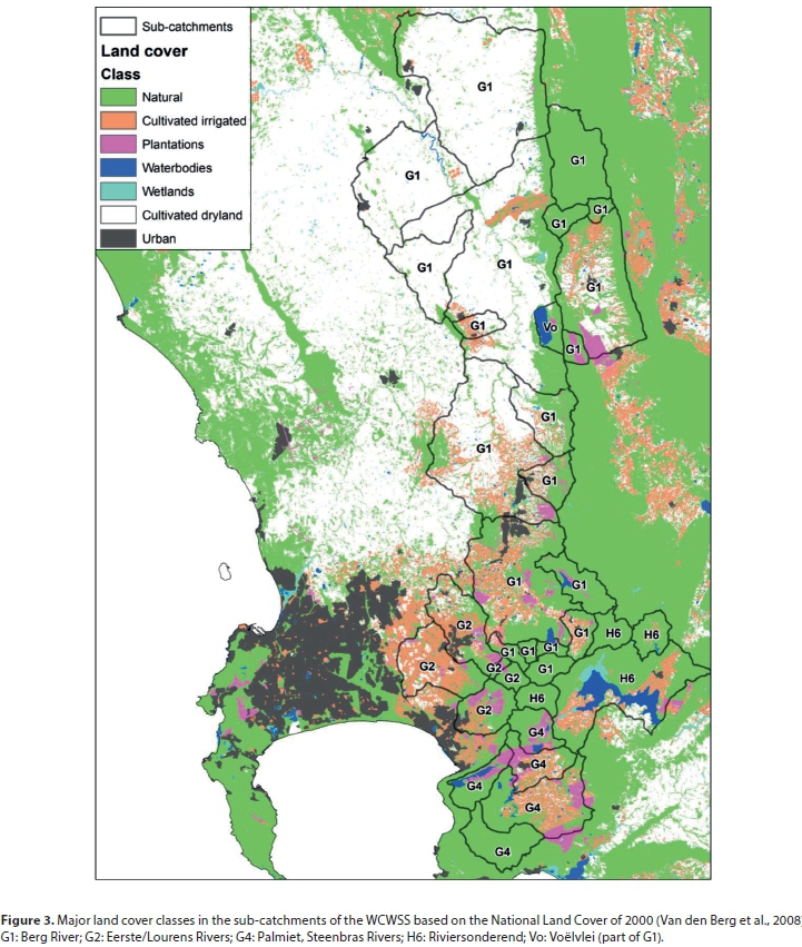
More than half of the total area of the WCWSS catchments has been transformed (Table 3, Fig. 3) into either dryland or irrigated agriculture, primarily vines and deciduous fruit. The catchments that are still mainly natural include the Riviersonderend, where most of the catchment above the Theewaterskloof Dam is still natural fynbos, and the Palmiet and Steenbras catchments in the Hottentots-Holland Nature Reserve, which are still mainly natural fynbos. Virtually all the valley floor and lower to middle slopes in the Berg River sub-catchments have been cultivated, so that only about 33.3% is still natural vegetation.

 

 

Alien plant invasions

In the 'Baseline' scenario, the condensed area of alien plant invasions was 22 190 ha or 5.5% of the natural vegetation of the WCWSS (Table 3), ranging from 8.6% in the Berg River to 3.3% of the Riviersonderend catchment (The condensed area is the equivalent dense area (i.e. 10 ha with 50% cover ≡ 5 condensed ha). Most of the invasions were not in in riparian areas or in areas where groundwater is accessible, with the latter (deep sandy soils) being most prevalent in the Berg and Riviersonderend catchments. The Berg River catchment has the most extensive riparian invasions (16.2% of the total) which occur along the Berg itself and along most of its tributaries, and are dominated by eucalypts and black wattle. Almost all the remaining natural vegetation in the WCWSS is invaded to some degree (Fig. 4). The most densely invaded areas are situated in the upper Berg and upper Riviersonderend catchments, particularly between Villiersdorp and Paarl (Fig. 4). This is important because this is also the portion of the WCWSS which gets the highest rainfall and generates most of the runoff (Fig. 2).

 

 

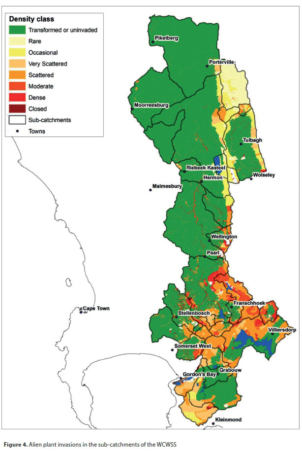
By 2045 with 'No management', the condensed invaded area equates to about 112 000 ha or 28.1% of the remaining natural vegetation (Table 3). The Berg River is the most invaded, with the condensed area being 50.8% of the natural vegetation, in other words a mean density of about 50%. The Riviersonderend catchment is the least invaded at 10.6%, mainly because it was less invaded than the Berg initially, but the invasions are concentrated in high runoff areas. The most extensive invasions are by pines which have a condensed area of about 11 000 ha in 2000 and a projected 70 000 ha in 2045.

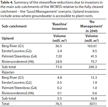
Flow reductions

The mean annual streamflow reductions for upland and riparian invasions in each of the sub-catchments are substantial, especially with 'No management' (Table 4). The greatest reductions for 'Baseline' upland invasions are found in the Berg and Riviersonderend sub-catchments with the total reductions for upland invasions coming to 71.0 mill. m³∙a⁻¹. Reductions due to riparian invasions are substantial in the Berg River, but much lower in the other catchments. With 'No management' the total reductions due to upland invasions increase substantially to 307 mill. m³∙a⁻¹, especially in the Berg River and Riviersonderend where they could increase 4.5 and 3.0 times, respectively (Table 4). Under 'No management', reductions due to riparian invasions also increase substantially to 16.8 mill. m³∙a⁻¹ (3.1 fold), with most of the reductions being found in the Berg River catchment. The relatively low increases in the Riviersonderend catchment are due mainly to the relatively low density of invasions in the 'Baseline' state (Table 3) which results in relatively low rates of increase in the density. The greater density of the invasions in the Berg River catchment leads to a more rapid increase in density and greater reductions under 'No management', emphasising the importance of controlling invasions at an early stage.

 

 

Stochastic yield reductions

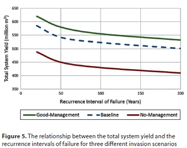
The stochastic analysis of the WCWSS outlined above demonstrate that the streamflow reductions for the 'Baseline' and 'No management' scenarios result in significant impacts on the WCWSS yield over the range failure recurrence intervals (Fig. 5). The yield for the 1:50 year recurrence interval of failure (98% assurance) is widely used in long-term planning for domestic supplies. At this level of assurance, the yields for the WCWSS are 580 mill. m³∙a⁻¹ for the 'Effective management', 542 mill. m³∙a⁻¹ for the 'Baseline' and 450 mill. m³∙a⁻¹ for the 'No management' scenarios. The 'Baseline' reduction of 38 mill. m³∙a⁻¹ is equivalent to losing two thirds of the capacity of Wemmershoek Dam every year, or 6.6% of the WCWSS yield of 580 mill. m³∙a⁻¹ at 98% assurance of supply. However, under the 'No management' scenario, the reduction increases to 130 mill. m³∙a⁻¹, which is 22.4% of the WCWSS yield, equivalent to losing the capacity of the Berg River Dam each year.

 

 

Spatial variability of yield reductions

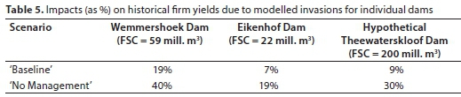
We examined the spatial variability of streamflow reduction impacts on yields within individual components of the WCWSS for the current and future invasion scenarios by determined the so-called 'historical firm yields' (HFYs) of three dams which are not affected by inter-catchment transfers for the period 1928-2005 (The HFY is determined by increasing the total abstractions in the modelled system by trial-and-error until the modelled system narrowly fails one year during the modelled historical period; i.e. the modelling is not performed in stochastic mode). This approach ensured that the modelled HFY impacts would be solely due to the modelled invasions in each dam's catchment, i.e., that interpretation of these modelled impacts would not be confounded by inter-catchment transfers. The three dams selected were Wemmershoek Dam in the Berg catchment, Eikenhof Dam in the Palmiet catchment and a hypothetical dam at the location of Theewaterskloof Dam in the Riviersonderend catchment. The reason for conducting this exercise for a hypothetical Theewaterskloof Dam is that, for the purposes of accommodating winter transfers of surplus inflows from the Berg River Dam into Theewaterskloof Dam, the operational full supply capacity (FSC) of the existing dam is about 200% larger than what the upstream catchment could sustain. The spatial differences of proportional impacts on yield due to invasive alien plant invasions (Table 5) are related primarily to a combination of two factors: the extent of invasions representing the 'Baseline' condition and the extent of invadable areas for the 'No management' condition.

 

 

Spatial variability of water supplies under scenarios of alien plant invasions

We also examined the long-term spatial variability of streamflow reduction impacts on average annual water supplies to individual water use sectors within individual components of the WCWSS for the 'Baseline' and 'No management' alien plant invasion scenarios for the period 1928-2005 hydrological years (Table 6). Given the close operational interactions between Theewaterskloof Dam and Berg River Dam, the outputs of the various modelled supply channels from these two dams to individual users were combined for the purposes of these calculations. For the same reason, the individual simulated supply volumes from Voëlvlei Dam and the Misverstand Weir on the Berg River were also combined. Furthermore, the various supply volumes for minor schemes and farm dams were combined by sub-region to enhance interpretation of the spatial variations of IAP impacts on average annual water supplies. For the complete WCWSS, the total mean annual impacts of IAPs on urban supplies (in absolute volume terms) far exceed the corresponding impacts on irrigation supplies (Table 6). The greatest modelled impact of IAPs on urban supplies (in absolute volume terms) is on water supplied from Wemmershoek Dam. Under 'No management' conditions IAPs could be expected to consume almost half of Wemmershoek's 98% assurance yield. The greatest modelled impact of IAPs on irrigation supplies (in absolute volume terms) is on water supplied from the combined Theewaterskloof and Berg River Dams.

 

DISCUSSION

This study clearly demonstrates that the reductions in streamflows as a result of the greater water-use of invading alien shrubs and trees can have substantial impacts on dam and system yields, even for the WCWSS which comprises several large dams. This confirms the findings of previous studies (Le Maitre and Görgens, 2003; Cullis et al., 2007). In this case the invasions are mainly in the headwater catchments (Fig. 4) and so have a significant impact on streamflows throughout the WCWSS and thus on the yields of each of the parts of the system and the whole WSS.

The fact that the reductions under the 'Baseline' invasions were already substantial, as well as the magnitude of the projected reductions, demonstrates why authorities need to take immediate action to clear catchments now rather than delaying action. If no actions are taken, or if they are delayed, then invasions rapidly increase in density and the costs of clearing increase. Although standard discounting approaches may make it seem less costly to develop alternative water sources, this is misleading. The impacts of alien plant invasions are not stationary so, unlike the finite yields from alternative schemes, the yields from invaded bulk water systems will decrease over time (Fig. 1) while the cost of clearing increases. The WCWSS is particularly vulnerable because all its water is supplied by invaded catchments, so that all parts of the WSS will experience reduced inflows and yields (Fig. 1), decreasing assurance of supply. All of the water that is available in the WCWSS catchments is already allocated to users or the ecological reserve, so the only way to increase the assurance of supply is by clearing invasions. Given this, there appears to be an inconsistency in the actions of the Department of Water and Sanitation. One the one hand, they use the provisions of the section of the National Water Act on Stream Flow Reduction Activities to restrict afforestation because of its impacts on stream flow (Dye and Versfeld, 2007). So, because the water resources in the WCWSS are already fully allocated, they would not have allowed further afforestation in the catchments supplying the WCWSS. Yet the Department seems to be unwilling to acknowledge that invasions by the same species used for forest plantations could be having similar impacts on runoff and, as we have demonstrated, the yields. In other words, they should be actively supporting clearing but are currently not doing so and it is not clear why this is the case.

Developing alternative schemes merely transfers the cost of dealing with invasions to future generations as there are no indications that technological advances will radically reduce clearing costs in the future. The severe water shortages currently being experienced by Cape Town and the neighbouring towns within the WCWSS demonstrate clearly that maintaining or increasing the yields of the existing WSS is critical for both immediate and long-term water security. The estimated current-day (Baseline) yield reduction of 38 mill. m³∙a⁻¹ could have provided Cape Town with about 54 days of water per year at 700 ML∙d⁻¹ had the invasions been cleared.

The results of the long-term studies of the hydrological impacts of plantations showed clearly that the reductions in low (dry season) flows are greater than those on annual flows (Scott and Smith, 1997), indicating a net depletion of catchment water storage. The depletion of catchment storage has been confirmed by other long-term studies where streamflow took time to recover after clearing (Scott and Lesch, 1997; Everson et al., 2014). These findings suggest that the effects of invasions are likely to be greatest during droughts, just when the maximum yield is required from the WSS. In addition, most of the invasions are in upland environments so, even if the invading plants are cleared, the depleted catchment storage will take time to replenish and reach levels where stream flows normalise again. This, in turn, makes a strong case for not waiting until droughts are underway before prioritising clearing.

At the moment, clearing in the WCWSS catchments is being funded almost entirely by the Extended Public Works Programme rather than directly by the water-users in the WCWSS. Although users are paying for their water, the funds raised by these levies are not being directly applied to environmental management in these catchments. Dedicated funding and monitoring of the clearing operation by those who pay is the best way to ensure that this is achieved. The simple message is that the sooner the water-users in the WCWSS invest in the clearing, including the use of biocontrol, the less it will cost them in total and the more they will benefit (Van Wilgen et al., 1997). By putting measures in place to ensure that the clearing is effective (Kraaij et al., 2017), they can ensure that this is a wise investment which will secure water supplies for them and for future generations. Although this study focused on the WCWSS, the same reasoning would apply to all water supply systems where the catchments have been invaded by species with similar hydrological impacts.

 

ACKNOWLEDGEMENTS

This study was funded by the Chief Directorate: Natural Resource Management of the Department of Environmental Affairs. We thank colleagues for comments and advice on the study and earlier drafts of the paper.

 

REFERENCES

BASTIAANSSEN WGM, MENENTI M, FEDDES RA and HOLTSLAG AAM (1998) A remote sensing surface energy balance algorithm for land (SEBAL). 1. Formulation. J. Hydrol. 212-213 198-212. https://doi.org/10.1016/S0022-1694(98)00253-4        [ Links ]

BIRKS HJB (1989) Holocene isochrone maps and patterns of tree-spreading in the British Isles. J. Biogeogr. 16 (6) 503. https://doi.org/10.2307/2845208        [ Links ]

BOSCH JM, VAN WILGEN BW and BANDS DP (1980) A model for comparing water yield from fynbos catchments burnt at different intervals. Water SA 4 191-196.         [ Links ]

BOSCH JM and VON GADOW K (1990) Regulating afforestation for water conservation in South Africa. S. Afr. For. J. 153 41-54. https://doi.org/10.1080/00382167.1990.9629032        [ Links ]

CALDER IR (1991) Water use by forests at the plot and catchment scale. Commonwealth For. Rev. 75 19-30.         [ Links ]

CULLIS JDS, GÖRGENS AHM and MARAIS C (2007) A strategic study of the impact of invasive alien plants in the high rainfall catchments and riparian zones of South Africa on total surface water yield. Water SA 33 35-42. https://doi.org/10.4314/wsa.v33i1.47869        [ Links ]

DWAF (2010) The Assessment of Water Availability in the Berg River Catchment (WMA 19) by means of Water Resource Related Models. Report No. 1. Summary Report. P WMA19/000/00/1209. DWAF Report No P WMA19/000/00/1209, Directorate National Water Resource Planning, Department of Water Affairs and Forestry, Pretoria.         [ Links ]

DWS (2014) WC WSS Reconciliation Strategy Status Report October 2014. Prepared by Umvoto Africa (Pty) Ltd in association with WorleyParsons on behalf of the Directorate: National Water Resource Planning, Department of Water and Sanitation, Pretoria.         [ Links ]

DYE P and JARMAIN C (2004) Water use by black wattle (Acacia mearnsii): implications for the link between removal of invading trees and catchment streamflow response. S. Afr. J. Sci. 100 40-44.         [ Links ]

DYE PJ and POULTER AG (1995) A field demonstration of the effect on streamflow of clearing of invasive pine and wattle trees from a riparian zone. S. Afr. For. J. 173 27-30. https://doi.org/10.1080/00382167.1995.9629687        [ Links ]

DYE P and VERSFELD D (2007) Managing the hydrological impacts of South African plantation forests: An overview. For. Ecol. Manage. 251 (1-2) 121-128. https://doi.org/10.1016/j.foreco.2007.06.013        [ Links ]

DZIKITI S, GUSH MB, LE MAITRE DC, MAHERRY A, JOVANOVIC NZ, RAMOELO A and CHO MA (2016) Quantifying potential water savings from clearing invasive alien Eucalyptus camaldulensis using in situ and high resolution remote sensing data in the Berg River Catchment, Western Cape, South Africa. For. Ecol. Manage. 361 69-80. https://doi.org/10.1016/j.foreco.2015.11.009        [ Links ]

DZIKITI S, SCHACHTSCHNEIDER K, NAIKEN V, GUSH M, MOSES G and LE MAITRE DC (2013) Water relations and the effects of clearing invasive Prosopis trees on groundwater in an arid environment in the Northern Cape, South Africa. J. Arid Environ. 90 (0) 103-113. https://doi.org/10.1016/j.jaridenv.2012.10.015        [ Links ]

DZVUKAMANJA TN, GÖRGENS AHM and JONKER V (2005) Streamflow reduction modelling in water resource analysis. WRC Report No. 1221/1/05. Water Research Commission, Pretoria.         [ Links ]

EVERSON CS, CLULOW AD, BECKER M, WATSON A, NGUBO C, BULCOCK H, MENGISTU M, LORENTZ S and DEMLIE M (2014) The long term impact of Acacia mearnsii trees on evaporation, streamflow, low flows and ground water resources. Phase II: Understanding the controlling environmental variables and soil water processes over a full crop rotation. WRC Report No. 2022/1/13. Water Research Commission, Pretoria.         [ Links ]

GELAND C, LE MAITRE D, FORSYTH G and LOCHNER P (2008) Review and Update of the Business Plan for Alien Plant Clearing in the Assegaaibos Catchment of the Berg River Dam. Report No. CSIR/CAS/EMS/ER/2008/0007/A, Consulting and Analytical Services, CSIR, Stellenbosch.         [ Links ]

HENGEVELD R (1989) Dynamics of Biological Invasions. Chapman and Hall, London.         [ Links ]

JARVIS PG and MCNAUGHTON KG (1986) Stomatal control of transpiration: scaling up from leaf to region. Adv. Ecol. Res. 12 1-49. https://doi.org/10.1016/S0065-2504(08)60119-1        [ Links ]

JONKER V, HAYES L and BEUSTER J (2007) The Assessment of Water Availability in the Berg Catchment (WMA 19) by Means of Water Resource Related Models. Report No. 2: Rainfall Data Preparation and MAP Surface. Report No P WMA19/000/00/0407, Prepared by Ninham Shand in association with Umvoto Africa, Department of Water Affairs and Forestry, South Africa.         [ Links ]

KRAAIJ T, BAARD JA, RIKHOTSO DR, COLE NS and VAN WILGEN BW (2017) Assessing the effectiveness of invasive alien plant management in a large fynbos protected area. Bothalia 47. https://doi.org/10.4102/abc.v47i2.2105        [ Links ]

LE MAITRE D, DZIKITI S and GUSH M (2016) Remote sensing data on evaporation for spatial and temporal extrapolation of site-specific data to landscapes and catchments. Report No. CSIR/NRE/ECOS/ER/2016/0019/B, Natural Resources and the Environment, CSIR, Stellenbosch.         [ Links ]

LE MAITRE D and GÖRGENS A (2003) Impact of invasive alien vegetation on dam yields. WRC Report No. KV 141/03b. Water Research Commission, Pretoria.         [ Links ]

LE MAITRE DC (2004) Predicting invasive species impacts on hydrological processes: the consequences of plant physiology for landscape processes. Weed Technol. 18 1408-1410. https://doi.org/10.1614/0890-037X(2004)018[1408:PISIOH]2.0.CO;2        [ Links ]

LE MAITRE DC, FORSYTH GG, DZIKITI S and GUSH MB (2013) Estimates of the impacts of invasive alien plants on water flows in South Africa. Report No. CSIR/NRE/ECO/ER/2013/0067/B. Natural Resources and the Environment, CSIR, Stellenbosch.         [ Links ]

LE MAITRE DC and GÖRGENS AHM (2001) Potential impacts of invasive alien plants on reservoir yields in South Africa. In: Tenth South African National Hydrology Symposium, 26-28 September 2001, Pietermaritzburg.         [ Links ]

LE MAITRE DC, GUSH MB and DZIKITI S (2015) Impacts of invading alien plant species on water flows at stand and catchment scales. AoB Plants 7 plv043. https://doi.org/10.1093/aobpla/plv043        [ Links ]

LE MAITRE DC, SCOTT DF and COLVIN C (1999) A review of information on interactions between vegetation and groundwater. Water SA 25 (2) 137-152.         [ Links ]

LE MAITRE DC, VAN WILGEN BW, CHAPMAN RA and MCKELLY D (1996) Invasive plants and water resources in the Western Cape Province, South Africa: modelling the consequences of a lack of management. J. Appl. Ecol. 33 (1) 161-172. https://doi.org/10.2307/2405025        [ Links ]

LE MAITRE DC, VAN WILGEN BW, GELDERBLOM CM, BAILEY C, CHAPMAN RA and NEL JA (2002) Invasive alien trees and water resources in South Africa: case studies of the costs and benefits of management. For. Ecol. Manage. 160 (1-3) 143-159. https://doi.org/10.1016/S0378-1127(01)00474-1        [ Links ]

LE MAITRE DC, VERSFELD DB and CHAPMAN RA (2000) The impact of invading alien plants on surface water resources in South Africa: a preliminary assessment. Water SA 26 397-408.         [ Links ]

LTSS (1972-2002) Land types of South Africa: Digital map (1:250 000 scale) and soil inventory databases. ARC-Institute for Soil, Climate and Water, Pretoria.         [ Links ]

MANZONI S, VICO G, KATUL G, PALMROTH S, JACKSON RB and PORPORATO A (2013) Hydraulic limits on maximum plant transpiration and the emergence of the safety-efficiency trade-off. New Phytol. 198 (1) 169-178. https://doi.org/10.1111/nph.12126        [ Links ]

MEIJNINGER WML and JARMAIN C (2014) Satellite-based annual evaporation estimates of invasive alien plant species and native vegetation in South Africa. Water SA 40 (1) 95-107. https://doi.org/10.4314/wsa.v40i1.12        [ Links ]

MULLER M, BISWAS A, MARTIN-HURTADO R, TORTAJADA C, GREY D and SADOFF CW (2015) WATER. Built infrastructure is essential. Science 349 (6248) 585-586. https://doi.org/10.1126/science.aac7606        [ Links ]

PRINSLOO FW and SCOTT DF (1999) Streamflow responses to the clearing of alien invasive trees from riparian zones at three sites in the Western Cape Province. South. Afr. For. J. 185 (185) 1-7. https://doi.org/10.1080/10295925.1999.9631220        [ Links ]

SCOTT DF (1993) Managing riparian zone vegetation to sustain streamflow: results of paired catchment experiments in South Africa. Can. J. For. Res. 29 (7) 1149-1157. https://doi.org/10.1139/x99-042        [ Links ]

SCOTT DF and LESCH W (1997) Streamflow responses to afforestation with Eucalyptus grandis and Pinus patula and to felling in the Mokobulaan experimental catchments, South Africa. J. Hydrol. 199 (3-4) 360-377. https://doi.org/10.1016/S0022-1694(96)03336-7        [ Links ]

SCOTT DF and SMITH RE (1997) Preliminary empirical models to predict reductions in total and low flows resulting from afforestation. Water SA 23 (2) 135-140.         [ Links ]

VAN DEN BERG EC, PLARRE C, VAN DEN BERG HM and THOMPSON MW (2008) The South African National Land Cover 2000. No. GW/A/2008/86, Agricultural Research Council (ARC) and Council for Scientific and Industrial Research (CSIR), Pretoria.         [ Links ]

VAN LILL WS, KRUGER FJ and VAN WYK DB (1980) Streamflow responses to afforestation with Eucalyptus grandis Hill Ex Maiden and Pinus patula Schlecht. Et Cham. on streamflow from experimental catchments at Mokobulaan, Traansvaal. J. Hydrol. 45 107-118. https://doi.org/10.1016/0022-1694(80)90069-4        [ Links ]

VAN NIEKERK PH and DU PLESSIS JA (2013) Unit reference value: Application in appraising inter-basin water transfer projects. Water SA 39 (4) 549-554. https://doi.org/10.4314/wsa.v39i4.14        [ Links ]

VAN WILGEN BW and LE MAITRE DC (2013) Rates of spread in invasive alien plants in South Africa. Report No: CSIR/NRE/ECOS/ER/2013/0107A. Natural Resources and the Environment CSIR, Stellenbosch.         [ Links ]

VAN WILGEN BW, LE MAITRE DC and COWLING RM (1998) Ecosystem services, efficiency, sustainability and equity: South Africa's Working for Water Programme. Trends Ecol. Evol. 13 (9) 378. https://doi.org/10.1016/S0169-5347(98)01434-7        [ Links ]

VAN WILGEN BW, LITTLE PR, CHAPMAN RA, GÖRGENS AHM, WILLEMS T and MARAIS C (1997) The sustainable development of water resources: History, financial costs, and benefits of alien plant control programmes. S. Afr. J. Sci. 93 (9) 404-411.         [ Links ]

VAN WILGEN BW, REYERS B, LE MAITRE DC, RICHARDSON DM and SCHONEGEVEL L (2008) A biome-scale assessment of the impact of invasive alien plants on ecosystem services in South Africa. J. Environ. Manage. 89 (4) 336-349. https://doi.org/10.1016/j.jenvman.2007.06.015        [ Links ]

VAN WYK DB (1987) Some impacts of afforestation on streamflow in the Western Cape Province, South Africa. Water SA 13 31-36.         [ Links ]

WHITEHEAD D and BEADLE CL (2004) Physiological regulation of productivity and water use in Eucalyptus: a review. For. Ecol. Manage. 193 (1-2) 113-140. https://doi.org/10.1016/j.foreco.2004.01.026        [ Links ]

 

 

Received 24 January 2018
Accepted in revised form 9 July 2019

 

 

* Corresponding author, email: dlmaitre@csir.co.za

^rND^sBASTIAANSSEN^nWGM^rND^sMENENTI^nM^rND^sFEDDES^nRA^rND^sHOLTSLAG^nAAM^rND^sBIRKS^nHJB^rND^sBOSCH^nJM^rND^sVAN WILGEN^nBW^rND^sBANDS^nDP^rND^sBOSCH^nJM^rND^sVON GADOW^nK^rND^sCALDER^nIR^rND^sCULLIS^nJDS^rND^sGÖRGENS^nAHM^rND^sMARAIS^nC^rND^sDYE^nP^rND^sJARMAIN^nC^rND^sDYE^nPJ^rND^sPOULTER^nAG^rND^sDYE^nP^rND^sVERSFELD^nD^rND^sDZIKITI^nS^rND^sGUSH^nMB^rND^sLE MAITRE^nDC^rND^sMAHERRY^nA^rND^sJOVANOVIC^nNZ^rND^sRAMOELO^nA^rND^sCHO^nMA^rND^sDZIKITI^nS^rND^sSCHACHTSCHNEIDER^nK^rND^sNAIKEN^nV^rND^sGUSH^nM^rND^sMOSES^nG^rND^sLE MAITRE^nDC^rND^sJARVIS^nPG^rND^sMCNAUGHTON^nKG^rND^sKRAAIJ^nT^rND^sBAARD^nJA^rND^sRIKHOTSO^nDR^rND^sCOLE^nNS^rND^sVAN WILGEN^nBW^rND^sLE MAITRE^nDC^rND^sLE MAITRE^nDC^rND^sGÖRGENS^nAHM^rND^sLE MAITRE^nDC^rND^sGUSH^nMB^rND^sDZIKITI^nS^rND^sLE MAITRE^nDC^rND^sSCOTT^nDF^rND^sCOLVIN^nC^rND^sLE MAITRE^nDC^rND^sVAN WILGEN^nBW^rND^sCHAPMAN^nRA^rND^sMCKELLY^nD^rND^sLE MAITRE^nDC^rND^sVAN WILGEN^nBW^rND^sGELDERBLOM^nCM^rND^sBAILEY^nC^rND^sCHAPMAN^nRA^rND^sNEL^nJA^rND^sLE MAITRE^nDC^rND^sVERSFELD^nDB^rND^sCHAPMAN^nRA^rND^sMANZONI^nS^rND^sVICO^nG^rND^sKATUL^nG^rND^sPALMROTH^nS^rND^sJACKSON^nRB^rND^sPORPORATO^nA^rND^sMEIJNINGER^nWML^rND^sJARMAIN^nC^rND^sMULLER^nM^rND^sBISWAS^nA^rND^sMARTIN-HURTADO^nR^rND^sTORTAJADA^nC^rND^sGREY^nD^rND^sSADOFF^nCW^rND^sPRINSLOO^nFW^rND^sSCOTT^nDF^rND^sSCOTT^nDF^rND^sSCOTT^nDF^rND^sLESCH^nW^rND^sSCOTT^nDF^rND^sSMITH^nRE^rND^sVAN LILL^nWS^rND^sKRUGER^nFJ^rND^sVAN WYK^nDB^rND^sVAN NIEKERK^nPH^rND^sDU PLESSIS^nJA^rND^sVAN WILGEN^nBW^rND^sLE MAITRE^nDC^rND^sCOWLING^nRM^rND^sVAN WILGEN^nBW^rND^sLITTLE^nPR^rND^sCHAPMAN^nRA^rND^sGÖRGENS^nAHM^rND^sWILLEMS^nT^rND^sMARAIS^nC^rND^sVAN WILGEN^nBW^rND^sREYERS^nB^rND^sLE MAITRE^nDC^rND^sRICHARDSON^nDM^rND^sSCHONEGEVEL^nL^rND^sVAN WYK^nDB^rND^sWHITEHEAD^nD^rND^sBEADLE^nCL^rND^1A01^nAdroit Takudzwa^sChakandinakira^rND^1A02^nTongayi^sMwedzi^rND^1A02^nTawanda^sTarakini^rND^1A03^nTaurai^sBere^rND^1A01^nAdroit Takudzwa^sChakandinakira^rND^1A02^nTongayi^sMwedzi^rND^1A02^nTawanda^sTarakini^rND^1A03^nTaurai^sBere^rND^1A01^nAdroit Takudzwa^sChakandinakira^rND^1A02^nTongayi^sMwedzi^rND^1A02^nTawanda^sTarakini^rND^1A03^nTaurai^sBere

RESEARCH PAPERS

 

Ecological responses of periphyton dry mass and epilithic diatom community structure for different atrazine and temperature scenarios

 

 

Adroit Takudzwa Chakandinakira^{I, *}; Tongayi Mwedzi^II; Tawanda Tarakini^II; Taurai Bere^III

^IDepartment of Geography, Bindura University of Science Education, P. Bag 1020, Bindura, Zimbabwe
^IIDepartment of Freshwater and Fishery Sciences, Chinhoyi University of Technology, Off Harare-Chirundu Rd, P Bag 7724, Chinhoyi, Zimbabwe
^IIIDepartment of Wildlife Ecology and Conservation, Chinhoyi University of Technology, Off Harare-Chirundu Rd, P Bag 7724, Chinhoyi, Zimbabwe

 

 

---

ABSTRACT

Climate change-induced temperature increase may influence the ecotoxicity of agricultural herbicides such as atrazine and consequently negatively impact aquatic biota. The objective of this study was to assess the effects of increased temperature on the ecotoxicity of atrazine to diatom community structure and stream periphyton load using laboratory microcosm experiments. A natural periphyton community from the Mukwadzi River, Zimbabwe, was inoculated into nine experimental systems containing clean glass substrates for periphyton colonisation. Communities were exposed to 0 µg∙L^-1 (control), 15 µg∙L^-1 and 200 µg∙L^-1 atrazine concentrations at 3 temperature levels of 26°C, 28°C and 30°C. Periphyton dry weight and community taxonomic composition were analysed on samples collected after 1, 2 and 3 weeks of colonisation. A linear mixed-effects model was used to analyse the main and interactive effects of atrazine and temperature on dry mass, species diversity, evenness and richness. Temperature and atrazine had significant additive effects on species diversity, richness and dry mass. As temperature increased, diatom species composition shifted from heat-sensitive species such as Achnanthidium affine to heat-tolerant species such as Achnanthidium exiguum and Epithemia adnata. Increasing temperature in aquatic environments contaminated with atrazine results in sensitive and temperature-intolerant diatoms being eliminated from periphyton communities. Climate change will exacerbate effects of atrazine on periphyton dry mass and diatom community structure.

Keywords: ecotoxicology, microcosm, biomonitoring, climate change

---

 

 

INTRODUCTION

The increase in agricultural activity and shift from traditional to chemical means of weed control has caused an increase in the contamination of water bodies by herbicides, consequently threatening aquatic biodiversity (Relyea, 2005). Increased use of agricultural herbicides such as atrazine has led to pollution of water bodies, thus leading to degradation of water quality (Villeneuve et al., 2011). Atrazine (2-chloro-4- (ethylamino)-6-s-triazine) is a triazine herbicide that inhibits photosynthesis through inhibiting electron transfer from photosystem II (PS II) by competing with the electron carrier molecule, plastoquinone (Shimabukuro and Swanson, 1969). Atrazine is mainly used for the control of annual broadleaf and grass weeds in agricultural production of maize. While atrazine has been banned in Europe, it is still widely used in other regions such as North America and Africa (Bethsass and Colangelo, 2006).

Periphyton communities (diatoms in particular) are good indicators of both climate change and water quality as they have highly resolved temporal sensitivity because of their short generation time and high sensitivity to nutrient input, organic pollution and chemical pollutants (Kilham et al., 1996; Bere and Chakandinakira, 2018). The response of periphyton to PS II inhibitors, such as atrazine, differs depending on the species, the effective herbicide concentration and the physiological state of algae (Guasch et al., 1998). Periphyton are confronted with anthropogenic-induced chemical stressors such as herbicides (Villeneuve et al., 2011) and physical stressors such as increased water temperature (Mahdy et al., 2015). Selection pressure (environmental conditions) may therefore result in susceptible diatom species being replaced by more resistant ones, thus affecting community structure as there would be reduced growth in other sensitive species (Blanck, 2002; Wood et al., 2016).

The toxicity of herbicides on periphyton in tropical regions is unknown as ecotoxicological testing is almost exclusively conducted in the temperate regions where water temperature ranges between 15°C and 24°C (Daam and Van Den Brink, 2010). Water temperatures as high as 28°C have been recorded in tropical rivers (Dallas, 2008) and, with the advent of climate change, higher temperatures are expected (Beilfuss, 2012). Projected increases in average annual temperatures for Southern Africa range from 1-4°C by 2050 (Daron, 2014). Although research on the interaction of temperature and atrazine has been conducted in temperate regions, applicability of the results could differ because of different climatic conditions (Baxter et al., 2016). For example, Zimbabwe's continental interior location means that it is predicted to warm even more rapidly than the global average (Ministry of Environment and Natural Resources Management, 2013). This potentially increases the interactive effect of temperature and atrazine.

It is expected that the use of pesticides will increase concomitantly with expected temperature changes, as warmer climates and climate extremes could be more favourable to the proliferation of insect and plant pests, and plant diseases (Kibria, 2014). Further to this, temperature is understood to have effects on the toxicity of pollutants including the persistent ones like atrazine. Previous studies have documented effects of increases in atrazine toxicity to catfish with temperature increase (Gaunt and Barker, 2000); lethality of the persistent organic pollutant dieldrin to the freshwater darter (Etheostoma nigrum) increased with increasing temperatures (Silbergeld, 1973); increase in mortality in juvenile rainbow trout exposed to the insecticide endosulfan as temperature was increased from 13°C to 16°C (Capkin et al., 2006); and toxicity of the insecticide carbaryl to the green frog increased with an increase in temperature (Boone and Bridges, 1999), among others (Lydy et al., 1999; Broomhall, 2002; Kibria, 2014; Landis et al., 2014). Vapouration of herbicides has been reported to be greater under tropical compared to temperate climates (Daam and Van Den Brink, 2010). The warmer climate also gives rise to faster breakdown of herbicide molecules in accordance with basic chemical reaction principles. The implications of these climate-induced changes on associated biota remain unknown (Bozinovic and Pörtner, 2015; Baxter et al., 2016). Quantifying such implications will help address water quality problems associated with the effect of climate change on the toxicity of aquatic pollutants. Such information should be available to increase adaptive capacity, thus reducing vulnerability where water management is concerned. More specifically, the effects of climate change on the toxicity of atrazine need to be quantified to implement informed conservation measures.

The cause-effect relationship, chain reactions and interactions between stressors and biota should be well understood for effective management of aquatic systems (Bere and Tundisi, 2011). These can be understood and interpreted using two hypotheses: (i) climate-induced toxicant sensitivity (CITS) hypothesis (Kimberly and Salice, 2014), where acclimation to altered climate parameters increases toxicant sensitivity, or (ii) toxicant-induced climate susceptibility (TICS), where toxicant exposure increases vulnerability to subsequent changes in climatic conditions (Hooper et al., 2013). This study employs microcosm experiments to explore the climate-induced toxicant sensitivity hypothesis for natural periphyton communities from tropical streams.

The aim of this study was to test the main and interactive effects of temperature and atrazine concentration on stream periphyton dry mass and epilithic diatom composition and community structure (diversity, evenness and richness). We endeavoured to explore: (i) the effect of different temperature scenarios on stream periphyton dry mass and epilithic diatom composition and community structure; (ii) the effect of atrazine on stream periphyton dry mass and epilithic diatom composition and community structure; and (iii) the interactive effect of different levels of temperature and atrazine on stream periphyton dry mass and epilithic diatom composition and community structure. We hypothesized that increases in temperature will result in an increase in the toxicity of atrazine by increasing the sensitivity of periphyton to atrazine and hence affect periphyton dry mass and epilithic diatom community structure and composition.

 

MATERIALS AND METHODS

Field periphyton collection

Periphyton were collected from the Mukwadzi River near Mapinga, Zimbabwe (17⁰26.369′E; 030⁰37.195′S). Water temperature in the river ranged from 19.3 ± 4.5 °C to 23.3 ± 3.7°C from January to August 2012 (Bere and Mangadze, 2014). The site water was tested for atrazine using liquid-liquid extraction (Yokley and Cheung, 2000) (Thermo Fisher Scientific, Waltham, MA, USA) and no trace of atrazine was found. Periphyton was sampled by scrubbing stones with a toothbrush in May 2016. Before sampling, the stones were gently shaken in the stream to remove loosely attached sediments and non-epilithic diatoms. The resulting biofilm suspension, making up a total of approximately 15 L, was pooled to form one sample that was put in plastic bottles. The biofilm suspension was then transported to the laboratory in a portable ice chest at the site water temperature where it was inoculated in the systems described in the section below.

Experimental setup and design

Experimental systems were set up to allow exposure of periphyton to stressors under controlled conditions in a laboratory. The experiment was conducted in the hot dry season (10-31 May 2016). A total of 9 microcosm experimental units (EUs) were established (Fig. 1a) following Bere and Tundisi (2011). Each EU consisted of 3 artificial streams made up of half-polyvinyl chloride (PVC) tubes measuring 90 × 14 × 8 cm that were connected in parallel to a 50 L tank (Bere and Tundisi, 2011). All systems were filled with Woods Hole culture medium prepared from distilled water (Nichols, 1973), modified by diluting 4 times, after Gold et al. (2003). This culture medium was kept without ethylenediaminetetraacetic acid (EDTA), which presents very high binding capacities for metals (Stauber and Florence, 1989), and supplemented with silica, an essential nutrient for diatom growth (Gold et al., 2003). A submersible pump (Aqua One P.R.C, Australia) allowed the continuous flow of water through each system at 10 mL∙s⁻¹, corresponding to a velocity of 0.2 cm∙s⁻¹

 

 

Each stream was fitted with 6 glass substrates (10 × 5 cm) in a slightly slanting position for periphyton colonization (Fig. 1a). Water level was kept at 0.5 cm above the highest end of the glass substrate. A light intensity of 55 ± 5 µmol∙s⁻¹∙m⁻² (falling in the range recommended by the international guidelines for ecotoxicological tests) (Nyholm and Källqvist, 1989; Laviale et al., 2010) at the water-air interface for photosynthetically active radiation (400-700 nm) was provided by fluorescent tubes with a light:dark regime of 12:12 h and measured using a Milwaukee Model SM700 light meter. In each EU, the required temperature was maintained by a submergible thermostat aquarium water heater (Via Aqua Commodity Inc., China) and measured using a thermometer after 1, 2 and 3 weeks. The systems were equilibrated overnight before the addition of epilithic diatom inoculum and atrazine (Detenbeck et al., 1996).

Atrazine exposure

Homogenised periphyton suspension from the field site was divided into 9 equal volumes of approximately 1.6 L corresponding to the number of EUs (control, low and high atrazine levels under 3 different temperature regimes). The schematic representation of the atrazine and temperature exposures used in this study is shown in Fig. 1b. Technical grade atrazine 500, with 47% atrazine, 3% other triazine and 50% other inert ingredients, supplied by Agricura Private Limited, Zimbabwe, was used to prepare the stock solutions by mixing it with wood culture medium and making sure that the solution was clear with no particulates.

Periphytic inoculum, in equal volumes, was introduced to the already thermoregulated EUs (Lambert et al., 2016). Atrazine stock solution was added to each EU with colonised periphyton after 24 h. Periphyton were exposed to 0 µg∙L⁻¹ (control), 15 µg∙L⁻¹ (low) and 200 µg∙L⁻¹ (high) of atrazine under 3 temperature levels, 26°C (T1), 28°C (T2) and 30°C (T3), for 3 weeks. Previous studies have used atrazine exposures ranging from a few hours to many weeks, but most use 2-21 days (Guasch et al., 1998; Brain et al., 2012). Spiked water samples (0, 15, 200 μg∙L⁻¹) were also analysed for determination of the actual atrazine concentrations, which were within 15% of the nominal values using a spectrophotometric method (Appendix, Table A1). The samples (100 mL) were extracted with two 10 mL portions of chloroform. The extract was then evaporated to dryness and the residue was dissolved in 25 mL of methanol. Aliquots were then analysed as described by Kesari and Gupta (1998). After every harvest (i.e. 1, 2 and 3 weeks after atrazine exposure), 10 L of stock solution were topped up in every EU to maintain a relatively constant exposure level and avoid nutrient depletion. There is little data on the concentration of atrazine in African water bodies, hence nominal concentrations were chosen as possible scenarios of herbicide concentration (Osibanjo et al., 2002). Intentionally high concentrations were selected in order to elicit a measurable response across all atrazine levels within the experimental duration.

Atrazine concentrations as high as 14.97 µg∙L⁻¹ were recorded in South Africa in the early 1990s (Pick et al., 1992; Ansara-Ross et al., 2012).In the 1990s, mean atrazine levels in Zimbabwe were reported to be 2.5 µg∙L⁻¹ and 97.7 µg∙L⁻¹ for rivers and lakes, respectively (Osibanjo et al., 2002). Information on the current status of atrazine levels in aquatic systems in Zimbabwe was not available, but the levels could be higher than those recorded by Osibanjo et al. (2002) given the approximately 6-fold increase in usage of herbicides for weed control in recent years (Mupako, Personal communication January 15, 2016). Other microcosm and artificial stream experiments have shown no effect of atrazine on periphyton at concentrations of up to 25 µg∙L⁻¹ (Lynch et al., 1985), while in another experiment the first effect was seen at 130 to 180 µg∙L⁻¹ (Jüttner et al., 1995). Atrazine concentrations greater than 100 µg∙L⁻¹ are considered to be high enough to cause dramatic effects on the photosynthesis, growth, chlorophyll content and biomass of most aquatic producers (Plumley and Davis, 1980; Kosinski and Merkle, 1984; Brockway et al., 1984; Wood et al., 2014). Thus, in this study, an atrazine level of 200 µg∙L⁻¹ was used as the 'high' treatment. Duration of exposure in natural streams is expected to be prolonged with increased use of atrazine. Hansson (1992) reports water temperature ranges of 15°C to 24°C in the temperate regions. However, water temperatures as high as 29.8°C have been recorded in Lake Kariba, and of 26°C in the Manyame Catchment, with projections of >30°C being expected by the middle of the 21^st century (Magadza, 2010; Bere and Mangadze, 2014). We therefore chose the high range of temperatures (i.e. 26°C C, 28°C and 30°C) to investigate plausible climate change scenarios in the tropics. The lowest temperature (i.e. 26°C) was identical to the temperature of the sampling site and defined as the reference temperature, and 28 and 30°C were the two thermic stress levels tested. Microcosms typically lack the complexity of whole ecosystems, such that features such as air-water and sediment-water exchanges, as well as the activities of wide-ranging organisms are not included. However, they are important in understanding and separating underlying mechanisms and the system can be controlled experimentally in a way that the actual world cannot (Schindler, 1998). Microcosms mimic natural freshwater streams and enable investigators to examine responses to perturbations from external to internal sources at the level of an integrated ecosystem and they also allow replication (Odum, 1984; Crossland and La Point, 1992).

Periphyton sampling and processing

Biofilms were collected after being exposed to atrazine for a period of 1, 2 and 3 weeks from two random glass substrates per stream. Periphyton was brushed with a toothbrush into mineral water (100 mL). After each sampling time, the artificial substrates were reset with a new glass substrate to maintain identical flow conditions (Bere and Tundisi, 2012).

Periphyton suspensions were homogenised by gently shaking and divided into two fractions (50 mL each) for epilithic diatom taxonomy and dry mass analysis. For diatom taxonomy, the subsample was cleaned of organic material using concentrated sulphuric acid and further cleaned with hydrogen peroxide as an oxidizing agent following Biggs and Kilroy (2000). Subsamples of cleaned diatom suspensions were pipetted onto 3 replicate coverslips and allowed to dry before being permanently mounted to slides using Pleurax (1.73 refractive index and manufactured by Dr JC Taylor). A minimum of 250 diatom valves were identified on each slide (based on counting efficiency method by Pappas and Stoermer (1996)) and were identified to species level using the guide by Taylor et al. (2007). The light compound microscope, Nilcon, Alphaphot 2, Type YS2-H, China, was used for identification.

The second fraction of the sample was used to measure dry mass, expressed in mg∙cm⁻². The sample was dispensed on pre-weighed and labelled Whatman GF/C: 1.2 µm 47 mm filter paper on a vacuum filtration unit. After filtration, the filter paper with the sample was oven-dried at 60°C for about 12 h until constant weight. This temperature is recommended to reduce the loss of some volatile organic compounds that can occur at higher temperatures (Aloi, 1990). The filter paper was reweighed to determine net dry weight mass of periphyton.

Data analysis

Principal component analysis (PCA) was used to show taxonomic differences in the different temperature and atrazine treatments using Paleontological Statistics (PAST) software Version 3.14 (Hammer et al., 2001). Taxa richness, Shannon Wiener diversity (H¹) and evenness metrics were also calculated in PAST. The effects of atrazine and temperature and their interaction on the different metrics and dry mass were tested by constructing linear mixed effects models (LMMs) while treating river identity nested in weeks as random variables using the ΄lme4΄ (Bates et al., 2011) package. To select appropriate models, full models were initially built having all independent variables (atrazine and temperature) and their interaction. The dredge function in package `MuMIn` (Barton, 2009) was used in selecting the best model. For the LMMs and model selection, the R statistical software (Version 3.4.1) (R Core Team, 2016) was used. The residuals for the LMMs were checked for normality and normality assumptions were not significantly violated.

 

RESULTS

Community composition

A total of 106 diatom species belonging to 44 genera were recorded during the course of the study. Ten dominant diatom species with mean relative abundances greater than 3% (Mahdy et al., 2015), and present in at least 2 communities, were described as characteristic of each diatom community developed throughout the experiment.

A shift in species composition was observed as Brachysira wygaschii Lange-Bertalot was present only at the lower temperature treatment of 26°C, while Staurosira elliptica (Schumann) Williams & Round and Pseudostaurosira brevistriata (Grunow in Van Heurk) Williams & Round appeared to be more temperature tolerant species as they were more prevalent in the higher temperature treatments of 28°C and 30°C. As atrazine concentration increased across all temperature treatments, relative abundance of diatoms reduced (Appendix, Table A2).

Principal component analysis Axis 1 and Axis 2 accounted for 77.51% total variation of the diatom data, with the first axis accounting for 68.65%. The principal component analysis separated diatom community structure mainly according to temperature treatment (Fig. 2). The T1 (26°C) temperature treatment, positively associated with the first axis, was associated with Fragilaria ulna (Nitzsch) Lange-Bertalot and Fragilaria biceps (Kutzing) Lange-Bertalot. The T2 (28°C) treatment was negatively associated with the first and second axis and was characterised by species such as Rhopalodia gibberula (Ehrenberg) O Müller, Achnanthidium crassum (Hustedt) Potapova & Ponader and Staurosira construens Ehrenberg. The T3 (30°C) treatments were negatively associated with Axis 1 and positively associated with Axis 2, being characterised by species such as Epithemia adnata (Kützing) Brébisson. PCA also clearly separated the diatom communities in relation to the different atrazine treatments. The control and low atrazine treatments were generally negatively associated with the second axis aggregating at the lower half of the PCA (which was also characterised by T1 and T2 temperature treatments). The high atrazine treatment was generally positively associated with Axis 2 being positioned at the top half of the PCA (which is also associated with the T3 temperature treatment) (Fig. 2).

 

EFFECTS OF TEMPERATURE AND ATRAZINE CONCENTRATION ON COMMUNITY STRUCTURE AND PERIPHYTON DRY MASS

As is represented by the models in Table A3 (Appendix), Shannon diversity index was significantly increased by the single effect of temperature increase (F = 4.3, d.f = 16, P < 0.05) and that of atrazine concentration (F = 19.08, d.f = 16, P < 0.001). However, the diversity was reduced when temperatures were increased under low atrazine concentrations, and was even lower under high atrazine concentrations (Fig. 3a). Likewise, species evenness was also significantly increased by increases in both temperature (P < 0.05) and atrazine concentration (P < 0.001). The increase in temperature under low and high atrazine concentrations had a negative effect on species evenness (Fig. 3b).

Dry mass was lower under conditions of increasing concentrations of atrazine (F = 79.08, d.f = 16, p < 0.001) and high at low temperatures (F = 52.5, d.f = 16, p < 0.001). High values of periphyton dry mass were produced at 26 and 28°C across the atrazine treatments (Fig. 4a, Table A3, Appendix) (F = 30.4, d.f = 16, p < 0.001). For all the LMMs, random effects of the week were relatively low (range 0.002-2.87), implying no temporal trends. Richness (Fig. 4b) was significantly reduced when both temperature (F = 9.84, d.f = 20, p < 0.001) and atrazine (F = 152.85, d.f = 20, p < 0.001) increased.

 

DISCUSSION

Effects of temperature on stream periphyton community structure.

Taxonomic analysis revealed a shift in epilithic diatom assemblage composition with increasing temperature. Increasing temperatures in control treatments selected for Achnanthidium exiguum (Grunow) Czarnecki and Epithemia adnata (Kützing) Brébisson which have known preferences for warm waters (Lambert et al., 2016). The elimination of temperature-sensitive diatom species and subsequent succession to temperature-tolerant species is in line with the CITS hypothesis. Linear mixed effects model results showed that richness and periphyton dry mass decreased with an increase in temperature, while Shannon diversity and evenness increased. This shows that temperature plays an important role in diatom ecology, as has been suggested by several studies (Patrick, 1971; Anderson, 2000; Di Pippo et al., 2012; Larras et al., 2013; Kimberly and Salice, 2014; Mahdy et al., 2015; Lambert et al., 2016). This study, therefore, demonstrates the statistical independence of temperature, as a controlling variable, from the other dominant variables.

Temperature increases (with the exception of the control treatment at 28°C) resulted in an increase in periphyton dry mass. Other studies have also made such observations; e.g., Mahdy et al. (2015) and Di Pippo et al. (2012) reported that at high temperatures (30°C) diatoms increase secretion of extracellular polymeric substances (EPSs - natural polymers of high molecular weight). EPSs are important in biofilm stability, constituting 50-90% of a biofilm's organic matter; hence the increase in measured dry mass (Donlan, 2002; Evans, 2003). Various authors have associated increases in EPS production at higher temperatures with coping with increased environmental stress (Vu et al., 2009; Lambert et al., 2016; Flemming, 2016).

Effects of atrazine on stream periphyton community structure

A shift in dominance of diatom communities was observed with an increase in atrazine concentration. High atrazine treatments of 200 µg∙L⁻¹ had the lowest species diversity and dry mass compared to the control and low atrazine treatments, because of photosynthetic inhibition that inhibited the accumulation of periphytic microalgal constituents and resulted in the elimination of sensitive species (Solomon et al., 1996).

Similarly to Detenbeck et al. (1996), in this study the effects of atrazine on periphyton accumulation were observed even from the lowest atrazine treatment levels of 15 µg∙L⁻¹. However, other microcosm and artificial stream experiments have shown no effect up to 25 µg∙L⁻¹ (Lynch et al., 1985) and the first effect at 130 to 180 µg∙L⁻¹ (Jüttner et al., 1995). This could be attributed to the absence of other environmental stressors, such as temperature, that were included in this study. Relative abundance of diatoms in this study did not differ at the various atrazine levels as was also found by Giddings et al. (2005) who used similar levels of atrazine (16 µg∙L⁻¹ and 145 µg∙L⁻¹). This means that streams that face contamination in our region are in danger of changes in biodiversity, productivity, energy fluxes, species assemblage compositions and food web dynamics, as diatoms which are part of the primary producers of the ecosystem are being affected. The present study suggests that atrazine has the potential to impair environmental quality and ecological health of surface waters and provides evidence for the need to regulate atrazine to avoid ecological implications.

Effect of temperature on the ecotoxicity of atrazine and resulting impact on periphyton community structure and productivity

The findings of this study regarding the main and interactive effects of atrazine and temperature are in agreement with many field observations (Wood et al., 2014; Patra et al., 2015). Kibria (2014) observed that at higher temperatures, the metabolism of aquatic organisms increases and oxygen concentration is reduced. Aerobic degradation of atrazine is therefore reduced at higher compared to lower temperatures, thereby prolonging PSII inhibition. Periphyton accumulation was significantly reduced by atrazine exposure at 26°C and further decline was observed in the atrazine-contaminated treatments as temperature increased, suggesting that the effect of atrazine increased with an increase in temperature. According to Kimberly and Salice (2014), changes in environmental conditions (e.g. temperature increase) can increase the vulnerability of populations or influence competition among algae. This also accounts for the changes in species diversity and species richness, as these decreased with an increase in temperature in the atrazine-contaminated sites.

Our results suggest that temperature increases the ecotoxicity of atrazine to periphyton, in line with CITS (as shown by the species diversity and richness models). Such interactions between temperature and atrazine are especially important in the face of climate change. Climate change-induced increases in temperature are therefore set to exacerbate the effects of atrazine on periphyton. As such, climate change poses a potential risk to algae atrazine exposure, and consequently entire ecosystems as periphyton are dominant primary producers. This is a real threat in anticipated temperature increases in southern Africa (Beilfuss, 2012). To act proactively and mitigate the consequences of climate change-induced herbicide toxicity, there should be controlled use of agricultural chemicals, monitoring of atrazine levels in water bodies and ecotoxicological testing of agricultural herbicides for accurate ecological risk assessments.

 

CONCLUSION

An increase in temperature appears to exacerbate the toxicity of atrazine to stream periphyton. The interaction of temperature and atrazine treatment was shown to reduce species richness and dry mass. The net effect of atrazine on periphyton will therefore depend on environmental conditions such as climate-induced temperature increase. The study provides evidence for the need to regulate atrazine for better adaptation to climate change, but we acknowledge the associated challenges. Furthermore, the findings of this study attest to the potential validity of periphyton, and more specifically epilithic diatoms, as potential indicators of atrazine contamination in a changing climate. National assessment of atrazine levels in Zimbabwean water systems can improve relevance and applicability of similar studies.

 

ACKNOWLEDGEMENTS

This study was made possible by the provision of funds by the British Ecological Society (BES; Grant No: 4218-5112) and International Foundation for Science (IFS; Grant No: W/4848−2). We are grateful to Chinhoyi University of Technology for the laboratories used to run the experiment and for laboratory equipment for the analysis of samples. We would also like to thank Dr N Chanza, Dr JC Taylor, Tinotenda Mangadze and Admire Chanyandura for their support during the course of this study.

 

REFERENCES

ALOI JE (1990) A critical review of recent freshwater periphyton field methods. Can. J. Fisheries Aquat. Sci. 47 (3) 656-670. https://doi.org/10.1139/f90-073        [ Links ]

ANDERSON NJ (2000) Miniview: Diatoms, temperature and climatic change. Eur. J. Phycol. 35 (4) 307-314. https://doi.org/10.1080/09670260010001735911        [ Links ]

ANSARA-ROSS T, WEPENER V, VAN DEN BRINK P and ROSS M (2012) Pesticides in South African fresh waters. Afr. J. Aquat. Sci. 37 (1) 1-16. https://doi.org/10.2989/16085914.2012.666336        [ Links ]

BARTON K (2009) Mumin: Multi-model inference. R package version 1. 0. 0. http://r-forge.r-project.org/projects/mumin/.         [ Links ]

BATES D, MAECHLER M and BOLKER B (2011) Lme4: Linear mixed-effects models using s4 classes. R package version 0.999375−39. URL: http://cran.R-project.Org/package=lme4        [ Links ]

BAXTER L, BRAIN RA, LISSEMORE L, SOLOMON KR, HANSON ML and PROSSER RS (2016) Influence of light, nutrients, and temperature on the toxicity of atrazine to the algal species Raphidocelis subcapitata: Implications for the risk assessment of herbicides. Ecotoxicol. Environ. Saf. 132 250-259. https://doi.org/10.1016/j.ecoenv.2016.06.022        [ Links ]

BEILFUSS R (2012) A risky climate for Southern African hydro: Assessing hydrological risks and consequences for Zambezi River basin dams. International Rivers, Berkeley, CA. 56 pp.         [ Links ]

BERE T and CHAKANDINAKIRA AT (2018) Diatoms as indicators of anthropogenic changes in water quality in Mucheke and Shagashe Rivers, Masvingo, Zimbabwe. In: Matsumura-Tundisi T and Tundisi JG (eds) Water Resources Management. Editora Scienza, São Carlos. https://doi.org/10.26626/978-85-5953-031-5.2018C001        [ Links ]

BERE T and MANGADZE T (2014) Diatom communities in streams draining urban areas: Community structure in relation to environmental variables. Trop. Ecol. 55 (2) 271-281.         [ Links ]

BERE T and TUNDISI J (2011) Toxicity and sorption kinetics of dissolved cadmium and Chromium III on tropical freshwater phytoperiphyton in laboratory mesocosm experiments. Sci. Total Environ. 409 (22) 4772-4780. https://doi.org/10.1016/j.scitotenv.2011.07.055        [ Links ]

BERE T and TUNDISI JG (2012) Effects of cadmium stress and sorption kinetics on tropical freshwater periphytic communities in indoor mesocosm experiments. Sci. Total Environ. 432 103-112. https://doi.org/10.1016/j.scitotenv.2012.05.084        [ Links ]

BETHSASS J and COLANGELO A (2006) European Union bans atrazine, while the United States negotiates continued use. Int. J. Occup. Environ. Health 12 (3) 260-267. https://doi.org/10.1179/oeh.2006.12.3.260        [ Links ]

BIGGS B and KILROY C (2000) Stream Periphyton Monitoring Manual. New Zealand Ministry for the Environment, New Zealand.         [ Links ]

BLANCK H (2002) A critical review of procedures and approaches used for assessing pollution-induced community tolerance (pict) in biotic communities. Hum. Ecol. Risk Assess. 8 (5) 1003-1034. https://doi.org/10.1080/1080-700291905792        [ Links ]

BOONE MD and BRIDGES CM (1999) The effect of temperature on the potency of carbaryl for survival of tadpoles of the green frog (Rana clamitans). Environ. Toxicol. Chem. 18 (7) 1482-1484. https://doi.org/10.1002/etc.5620180720        [ Links ]

BOZINOVIC F and PÖRTNER HO (2015) Physiological ecology meets climate change. Ecol. Evol. 5 (5) 1025-1030. https://doi.org/10.1002/ece3.1403        [ Links ]

BRAIN RA, HOBERG J, HOSMER AJ and WALL SB (2012) Influence of light intensity on the toxicity of atrazine to the submerged freshwater aquatic macrophyte Elodea canadensis. Ecotoxicol. Environ. Saf. 79 55-61. https://doi.org/10.1016/j.ecoenv.2011.12.001        [ Links ]

BROCKWAY DL, SMITH PD and STANCIL FE (1984) Fate and effects of atrazine in small aquatic microcosms. Bull. Environ. Contam. Toxicol. 32 (1) 345-353. https://doi.org/10.1007/BF01607508        [ Links ]

BROOMHALL S (2002) The effects of endosulfan and variable water temperature on survivorship and subsequent vulnerability to predation in Litoria citropa tadpoles. Aquat. Toxicol. 61 (3-4) 243-250. https://doi.org/10.1016/S0166-445X(02)00061-9        [ Links ]

CAPKIN E, ALTINOK I and KARAHAN S (2006) Water quality and fish size affect toxicity of endosulfan, an organochlorine pesticide, to rainbow trout. Chemosphere 64 (10) 1793-1800. https://doi.org/10.1016/j.chemosphere.2005.12.050        [ Links ]

CROSSLAND NO and LA POINT TW (1992) The design of mesocosm experiments. Environ. Toxicol. Chem. 11 (1) 1-4. https://doi.org/10.1002/etc.5620110101        [ Links ]

DAAM MA and VAN DEN BRINK PJ (2010) Implications of differences between temperate and tropical freshwater ecosystems for the ecological risk assessment of pesticides. Ecotoxicology 19 (1) 24-37. https://doi.org/10.1007/s10646-009-0402-6        [ Links ]

DALLAS H (2008) Water temperature and riverine ecosystems: An overview of knowledge and approaches for assessing biotic responses, with special reference to South Africa. Water SA 34 (3) 393-404. https://doi.org/10.4314/wsa.v34i3.180634        [ Links ]

DARON J (2014) Regional climate messages: Southern Africa. Scientific report from the CARIAA Adaptation at Scale in Semi-Arid Regions (ASSAR) project, December 2014.         [ Links ]

DETENBECK NE, HERMANUTZ R, ALLEN K and SWIFT MC (1996) Fate and effects of the herbicide atrazine in flow‐through wetland mesocosms. Environ. Toxicol. Chem. 15 (6) 937-946. https://doi.org/10.1002/etc.5620150616        [ Links ]

DI PIPPO F, ELLWOOD NTW, GUZZON A, SILIATO L, MICHELETTI E, DE PHILIPPIS R and ALBERTANO PB (2012) Effect of light and temperature on biomass, photosynthesis and capsular polysaccharides in cultured phototrophic biofilms. J. Appl. Phycol. 24 (2) 211-220. https://doi.org/10.1007/s10811-011-9669-0        [ Links ]

DONLAN RM (2002) Biofilms: Microbial life on surfaces. Emerg. Infect. Dis. 8 (9). https://doi.org/10.3201/eid0809.020063        [ Links ]

EVANS LV (2003) Biofilms: Recent Advances in their Study and Control. CRC Press, Boca Raton.         [ Links ]

FLEMMING H-C (2016) Eps-then and now. Microorganisms 4 (4) 41. https://doi.org/10.3390/microorganisms4040041        [ Links ]

GAUNT P and BARKER SA (2000) Matrix solid phase dispersion extraction of triazines from catfish tissues; examination of the effects of temperature and dissolved oxygen on the toxicity of atrazine. Int. J. Environ. Pollut. 13 (1-6) 284-312. https://doi.org/10.1504/IJEP.2000.002320        [ Links ]

GIDDINGS JM, ANDERSON TA, HALL LW JR, KENDALL RJ, RICHARDS RP, SOLOMON KR, and WILLIAMS WM (2005) A Probabilistic aquatic ecological risk assessment of atrazine in North American surface waters. SETAC, Pensacola, FL, USA.         [ Links ]

GOLD C, FEURTET‐MAZEL A, COSTE M and BOUDOU A (2003) Effects of cadmium stress on periphytic diatom communities in indoor artificial streams. Freshwater Biol. 48 (2) 316-328. https://doi.org/10.1046/j.1365−2427.2003.00980.x        [ Links ]

GUASCH H, IVORRA N, LEHMANN V, PAULSSON M, REAL M and SABATER S (1998) Community composition and sensitivity of periphyton to atrazine in flowing waters: The role of environmental factors. J. Appl. Phycol. 10 (2) 203-213. https://doi.org/10.1023/A:1008035212208        [ Links ]

HAMMER O, HARPER D and RYAN P (2001) Past (paleontological statistics) version 3.14. Software package for education and data analysis. Paleontol. Electrón. 4 (1) 9 pp.         [ Links ]

HANSSON L (1992) Factors regulating periphytic algal biomass. Limnol. Oceanogr. 37 (2) 322-328. https://doi.org/10.4319/lo.1992.37.2.0322        [ Links ]

HOOPER MJ, ANKLEY GT, CRISTOL DA, MARYOUNG LA, NOYES PD and PINKERTON KE (2013) Interactions between chemical and climate stressors: A role for mechanistic toxicology in assessing climate change risks. Environ. Toxicol. Chem. 32 (1) 32-48. https://doi.org/10.1002/etc.2043        [ Links ]

JÜTTNER I, PEITHER A, LAY J, KETTRUP A and ORMEROD S (1995) An outdoor mesocosm study to assess ecotoxicological effects of atrazine on a natural plankton community. Arch. Environ. Contam. Toxicol. 29 (4) 435-441. https://doi.org/10.1007/BF00208371        [ Links ]

KESARI R and GUPTA V (1998) A simple method for the spectrophotometric determination of atrazine using p-aminoacetophenone and its application in environmental and biological samples. Talanta 47 (5) 1085-1092. https://doi.org/10.1016/S0039-9140(98)00168-4        [ Links ]

KIBRIA G (2014) Climate change and chemical contaminants. URL: https://www.researchgate.net/publication/261216780_Climate_Change_and_Chemical_Contaminants        [ Links ]

KILHAM SS, THERIOT EC and FRITZ SC (1996) Linking planktonic diatoms and climate change in the large lakes of the yellowstone ecosystem using resource theory. Limnol. Oceanogr. 41 (5) 1052-1062. https://doi.org/10.4319/lo.1996.41.5.1052        [ Links ]

KIMBERLY DA and SALICE CJ (2014) Complex interactions between climate change and toxicants: Evidence that temperature variability increases sensitivity to cadmium. Ecotoxicology 23 (5) 809-817. https://doi.org/10.1007/s10646-014−1221-y        [ Links ]

KOSINSKI RJ and MERKLE MG (1984) The effect of four terrestrial herbicides on the productivity of artificial stream algal communities. J. Environ. Qual. 13 (1) 75-82. https://doi.org/10.2134/jeq1984.00472425001300010014x        [ Links ]

LAMBERT AS, DABRIN A, MORIN S, GAHOU J, FOULQUIER A, COQUERY M and PESCE S (2016) Temperature modulates phototrophic periphyton response to chronic copper exposure. Environ. Pollut. 208 821-829. https://doi.org/10.1016/j.envpol.2015.11.004        [ Links ]

LANDIS WG, ROHR JR, MOE SJ, BALBUS JM, CLEMENTS W, FRITZ A, HELM R, HICKEY C, HOOPER M and STAHL RG (2014) Global climate change and contaminants, a call to arms not yet heard? Integr. Environ. Assess. Manage. 10 (4) 483-484. https://doi.org/10.1002/ieam.1568        [ Links ]

LARRAS F, LAMBERT A-S, PESCE S, RIMET F, BOUCHEZ A and MONTUELLE B (2013) The effect of temperature and a herbicide mixture on freshwater periphytic algae. Ecotoxicol. Environ. Saf. 98 162-170. https://doi.org/10.1016/j.ecoenv.2013.09.007        [ Links ]

LAVIALE M, PRYGIEL J and CRÉACH A (2010) Light modulated toxicity of isoproturon toward natural stream periphyton photosynthesis: A comparison between constant and dynamic light conditions. Aquat. Toxicol. 97 (4) 334-342. https://doi.org/10.1016/j.aquatox.2010.01.004        [ Links ]

LYDY MJ, BELDEN J and TERNES M (1999) Effects of temperature on the toxicity of m-parathion, chlorpyrifos, and pentachlorobenzene to Chironomus tentans. Arch. Environ. Contam. Toxicol. 37 (4) 542-547. https://doi.org/10.1007/s002449900550        [ Links ]

LYNCH TR, JOHNSON HE and ADAMS WJ (1985) Impact of atrazine and hexachlorobiphenyl on the structure and function of model stream ecosystems. Environ. Toxicol. Chem. 4 (3) 399-413. https://doi.org/10.1002/etc.5620040315        [ Links ]

MAGADZA C (2010) Environmental state of Lake Kariba and Zambezi River valley: Lessons learned and not learned. Lakes Reservoirs Res. Manage. 15 (3) 167-192. https://doi.org/10.1111/j.1440−1770.2010.00438.x        [ Links ]

MAHDY A, HILT S, FILIZ N, BEKLIOĞLU M, HEJZLAR J, ÖZKUNDAKCI D, PAPASTERGIADOU E, SCHARFENBERGER U, ŠORF M and STEFANIDIS K (2015) Effects of water temperature on summer periphyton biomass in shallow lakes: A pan-European mesocosm experiment. Aquat. Sci. 77 (3) 499-510. https://doi.org/10.1007/s00027-015-0394-7        [ Links ]

MINISTRY OF ENVIRONMENT AND NATURAL RESOURCES MANAGEMENT (2013) Zimbabwe National Climate Change Response Strategy (first draft). Harare, Zimbabwe: Government of Zimbabwe.         [ Links ]

MUPAKO K (2016) Personal communication, 15 January 2016. Sales manager, Agricura Chinhoyi Branch, 137, Midway St, Chinhoyi, Zimbabwe.         [ Links ]

NICHOLS HW (1973) Growth media-freshwater. In: Handbook of Phycological Methods: Culture Methods and Growth Measurements. 7-24.         [ Links ]

NYHOLM N and KÄLLQVIST T (1989) Methods for growth inhibition toxicity tests with freshwater algae. Environ. Toxicol. Chem. 8 (8) 689-703. https://doi.org/10.1002/etc.5620080807        [ Links ]

ODUM EP (1984) The mesocosm. BioScience 34 (9) 558-562. https://doi.org/10.2307/1309598        [ Links ]

OSIBANJO O, BOUWMAN H, BASHIR N, OKOND'AHOKA J, CHOONG KWET YVE R and ONYOYO H (2002) Regionally based assessment of persistent toxic substances. Sub-saharan Africa regional report. UNEP Chemicals, Geneva.         [ Links ]

PAPPAS JL and STOERMER EF (1996) Quantitative method for determining a representative algal sample count 1. J. Phycol. 32 (4) 693-696. https://doi.org/10.1111/j.0022−3646.1996.00693.x        [ Links ]

PATRA RW, CHAPMAN JC, LIM RP, GEHRKE PC and SUNDERAM RM (2015) Interactions between water temperature and contaminant toxicity to freshwater fish. Environ. Toxicol. Chem. 34 (8) 1809-1817. https://doi.org/10.1002/etc.2990        [ Links ]

PATRICK R (1971) The effects of increasing light and temperature on the structure of diatom communities. Limnol. Oceanogr. 16 (2) 405-421. https://doi.org/10.4319/lo.1971.16.2.0405        [ Links ]

PICK FE, VAN DYK LP and BOTHA E (1992) Atrazine in ground and surface water in maize production areas of the Transvaal, South Africa. Chemosphere 25 (3) 335-341. https://doi.org/10.1016/0045-6535(92)90550-B        [ Links ]

PLUMLEY FG and DAVIS DE (1980) The effects of a photosynthesis inhibitor atrazine, on salt marsh edaphic algae, in culture, microecosystems, and in the field. Estuaries 3 (4) 271-277. https://doi.org/10.2307/1352082        [ Links ]

R CORE TEAM (2016) R: A language and environment for statistical computing. Vienna, Austria. Retrieved from https://www.R-project.org/        [ Links ]

RELYEA RA (2005) The impact of insecticides and herbicides on the biodiversity and productivity of aquatic communities. Ecol. Appl. 15 (2) 618-627. https://doi.org/10.1890/03-5342        [ Links ]

SHIMABUKURO RH and SWANSON HR (1969) Atrazine metabolism, selectivity, and mode of action. J. Agric. Food Chem. 17 (2) 199-205. https://doi.org/10.1021/jf60162a044        [ Links ]

SILBERGELD EK (1973) Dieldrin. Effects of chronic sublethal exposure on adaptation to thermal stress in fresh water fish. Environ. Sci. Technol. 7 (9) 846-849. https://doi.org/10.1021/es60081a010        [ Links ]

SOLOMON KR, BAKER DB, RICHARDS RP, DIXON KR, KLAINE SJ, LA POINT TW, KENDALL RJ, WEISSKOPF CP, GIDDINGS JM and GIESY JP (1996) Ecological risk assessment of atrazine in North American surface waters. Environ. Toxicol. Chem. 15 (1) 31-76. https://doi.org/10.1002/etc.5620150105        [ Links ]

TAYLOR JC, HARDING WR and ARCHIBALD C (2007) An illustrated guide to some common diatom species from South Africa. WRC Report No. TT 282/07. Water Research Commission, Pretoria.         [ Links ]

VILLENEUVE A, HUMBERT J and LARROUDÉ S (2011) Herbicide Contamination of Freshwater Ecosystems: Impact on Microbial Communities: IntechOpen.URL: https://www.intechopen.com/books/pesticides-formulations-effects-fate/herbicide-contamination-of-freshwater-ecosystems-impact-on-microbial-communities.         [ Links ]

VU B, CHEN M, CRAWFORD RJ and IVANOVA EP (2009) Bacterial extracellular polysaccharides involved in biofilm formation. Molecules 14 (7) 2535-2554. https://doi.org/10.3390/molecules14072535        [ Links ]

WOOD RJ, MITROVIC SM and KEFFORD BJ (2014) Determining the relative sensitivity of benthic diatoms to atrazine using rapid toxicity testing: A novel method. Sci. Total Environ. 485 421-427. https://doi.org/10.1016/j.scitotenv.2014.03.115        [ Links ]

WOOD RJ, MITROVIC SM, LIM RP and KEFFORD BJ (2016) The influence of reduced light intensity on the response of benthic diatoms to herbicide exposure. Environ. Toxicol. Chem. 35 (9) 2252-2260. doi: 10.1002/etc.3379 https://doi.org/10.1002/etc.3379        [ Links ]

YOKLEY RA and CHEUNG MW (2000) Analytical method for the determination of atrazine and its dealkylated chlorotriazine metabolites in water using gas chromatography/mass selective detection. J. Agric. Food Chem. 48 (10) 4500-4507. https://doi.org/10.1021/jf991100v        [ Links ]

 

 

Received 22 May 2018
Accepted in revised form 20 September 2019

 

 

* Corresponding author, email: chakandinakirat@gmail.com

 

 

 

 

Table A2 - Click to enlarge

 

 

Table A3 - Click to enlarge

^rND^sALOI^nJE^rND^sANDERSON^nNJ^rND^sANSARA-ROSS^nT^rND^sWEPENER^nV^rND^sVAN DEN BRINK^nP^rND^sROSS^nM^rND^sBAXTER^nL^rND^sBRAIN^nRA^rND^sLISSEMORE^nL^rND^sSOLOMON^nKR^rND^sHANSON^nML^rND^sPROSSER^nRS^rND^sBERE^nT^rND^sCHAKANDINAKIRA^nAT^rND^sBERE^nT^rND^sMANGADZE^nT^rND^sBERE^nT^rND^sTUNDISI^nJ^rND^sBERE^nT^rND^sTUNDISI^nJG^rND^sBETHSASS^nJ^rND^sCOLANGELO^nA^rND^sBLANCK^nH^rND^sBOONE^nMD^rND^sBRIDGES^nCM^rND^sBOZINOVIC^nF^rND^sPÖRTNER^nHO^rND^sBRAIN^nRA^rND^sHOBERG^nJ^rND^sHOSMER^nAJ^rND^sWALL^nSB^rND^sBROCKWAY^nDL^rND^sSMITH^nPD^rND^sSTANCIL^nFE^rND^sBROOMHALL^nS^rND^sCAPKIN^nE^rND^sALTINOK^nI^rND^sKARAHAN^nS^rND^sCROSSLAND^nNO^rND^sLA POINT^nTW^rND^sDAAM^nMA^rND^sVAN DEN BRINK^nPJ^rND^sDALLAS^nH^rND^sDETENBECK^nNE^rND^sHERMANUTZ^nR^rND^sALLEN^nK^rND^sSWIFT^nMC^rND^sDI PIPPO^nF^rND^sELLWOOD^nNTW^rND^sGUZZON^nA^rND^sSILIATO^nL^rND^sMICHELETTI^nE^rND^sDE PHILIPPIS^nR^rND^sALBERTANO^nPB^rND^sDONLAN^nRM^rND^sFLEMMING^nH-C^rND^sGAUNT^nP^rND^sBARKER^nSA^rND^sGOLD^nC^rND^sFEURTET‐MAZEL^nA^rND^sCOSTE^nM^rND^sBOUDOU^nA^rND^sGUASCH^nH^rND^sIVORRA^nN^rND^sLEHMANN^nV^rND^sPAULSSON^nM^rND^sREAL^nM^rND^sSABATER^nS^rND^sHAMMER^nO^rND^sHARPER^nD^rND^sRYAN^nP^rND^sHANSSON^nL^rND^sHOOPER^nMJ^rND^sANKLEY^nGT^rND^sCRISTOL^nDA^rND^sMARYOUNG^nLA^rND^sNOYES^nPD^rND^sPINKERTON^nKE^rND^sJÜTTNER^nI^rND^sPEITHER^nA^rND^sLAY^nJ^rND^sKETTRUP^nA^rND^sORMEROD^nS^rND^sKESARI^nR^rND^sGUPTA^nV^rND^sKILHAM^nSS^rND^sTHERIOT^nEC^rND^sFRITZ^nSC^rND^sKIMBERLY^nDA^rND^sSALICE^nCJ^rND^sKOSINSKI^nRJ^rND^sMERKLE^nMG^rND^sLAMBERT^nAS^rND^sDABRIN^nA^rND^sMORIN^nS^rND^sGAHOU^nJ^rND^sFOULQUIER^nA^rND^sCOQUERY^nM^rND^sPESCE^nS^rND^sLANDIS^nWG^rND^sROHR^nJR^rND^sMOE^nSJ^rND^sBALBUS^nJM^rND^sCLEMENTS^nW^rND^sFRITZ^nA^rND^sHELM^nR^rND^sHICKEY^nC^rND^sHOOPER^nM^rND^sSTAHL^nRG^rND^sLARRAS^nF^rND^sLAMBERT^nA-S^rND^sPESCE^nS^rND^sRIMET^nF^rND^sBOUCHEZ^nA^rND^sMONTUELLE^nB^rND^sLAVIALE^nM^rND^sPRYGIEL^nJ^rND^sCRÉACH^nA^rND^sLYDY^nMJ^rND^sBELDEN^nJ^rND^sTERNES^nM^rND^sLYNCH^nTR^rND^sJOHNSON^nHE^rND^sADAMS^nWJ^rND^sMAGADZA^nC^rND^sMAHDY^nA^rND^sHILT^nS^rND^sFILIZ^nN^rND^sBEKLIOĞLU^nM^rND^sHEJZLAR^nJ^rND^sÖZKUNDAKCI^nD^rND^sPAPASTERGIADOU^nE^rND^sSCHARFENBERGER^nU^rND^sŠORF^nM^rND^sSTEFANIDIS^nK^rND^sNICHOLS^nHW^rND^sNYHOLM^nN^rND^sKÄLLQVIST^nT^rND^sODUM^nEP^rND^sPAPPAS^nJL^rND^sSTOERMER^nEF^rND^sPATRA^nRW^rND^sCHAPMAN^nJC^rND^sLIM^nRP^rND^sGEHRKE^nPC^rND^sSUNDERAM^nRM^rND^sPATRICK^nR^rND^sPICK^nFE^rND^sVAN DYK^nLP^rND^sBOTHA^nE^rND^sPLUMLEY^nFG^rND^sDAVIS^nDE^rND^sRELYEA^nRA^rND^sSHIMABUKURO^nRH^rND^sSWANSON^nHR^rND^sSILBERGELD^nEK^rND^sSOLOMON^nKR^rND^sBAKER^nDB^rND^sRICHARDS^nRP^rND^sDIXON^nKR^rND^sKLAINE^nSJ^rND^sLA POINT^nTW^rND^sKENDALL^nRJ^rND^sWEISSKOPF^nCP^rND^sGIDDINGS^nJM^rND^sGIESY^nJP^rND^sVU^nB^rND^sCHEN^nM^rND^sCRAWFORD^nRJ^rND^sIVANOVA^nEP^rND^sWOOD^nRJ^rND^sMITROVIC^nSM^rND^sKEFFORD^nBJ^rND^sWOOD^nRJ^rND^sMITROVIC^nSM^rND^sLIM^nRP^rND^sKEFFORD^nBJ^rND^sYOKLEY^nRA^rND^sCHEUNG^nMW^rND^1A01^nEmmanuel^sGakuba^rND^1A01^nBrenda^sMoodley^rND^1A01 A02^nPatrick^sNdungu^rND^1A03^nGrace^sBirungi^rND^1A01^nEmmanuel^sGakuba^rND^1A01^nBrenda^sMoodley^rND^1A01 A02^nPatrick^sNdungu^rND^1A03^nGrace^sBirungi^rND^1A01^nEmmanuel^sGakuba^rND^1A01^nBrenda^sMoodley^rND^1A01 A02^nPatrick^sNdungu^rND^1A03^nGrace^sBirungi

RESEARCH PAPERS

 

Evaluation of persistent organochlorine pesticides and polychlorinated biphenyls in Umgeni River bank soil, KwaZulu-Natal, South Africa

 

 

Emmanuel Gakuba^I; Brenda Moodley^{I, *}; Patrick Ndungu^{I, II}; Grace Birungi^III

^ISchool of Chemistry and Physics, University of KwaZulu-Natal, Westville Campus, Private Bag x54001, Durban 4000, South Africa
^IIDepartment of Applied Chemistry, Doornfontein Campus, University of Johannesburg, PO Box 17011, Doornfontein 2028, Johannesburg, South Africa
^IIIChemistry Department, College of Science, Mbarara University of Science and Technology, PO Box 1410, Mbarara, Uganda

 

 

---

ABSTRACT

This study investigated the presence and distribution of organochlorine pesticides (OCPs) and polychlorinated biphenyls (PCBs) in soil collected along the banks of the Umgeni River, one of the largest rivers in the province of KwaZulu-Natal, South Africa. The analysis was performed using gas chromatography-mass spectrometry (GC-MS). The results showed that the levels of OCPs ranged from 3.58±0.09 ng/g for hexachlorobenzene (HCB) to 82.65±2.82 ng/g for HCH, with an individual mean concentration of 24.33±2.00 ng/g dry weight (dw). The levels of PCBs ranged from 10.46 ng/g for PCB105 to 89.46 ng/g for PCB180, with an average PCB value of 25.47±1.26 ng/g, dw. The highest levels of OCPs and PCBs were found at Northern Wastewater Treatment Plant (mean OCP: 32.39±3.97 ng/g and PCB: 67.87±1.67 ng/g). The two most abundant contaminants in the river were endrin and PCB180.

Keywords: Umgeni River, bank soil, OCPs, PCBs, gas chromatography mass spectrometry

---

 

 

INTRODUCTION

Organochlorine pesticides (OCPs), such as aldrin, endrin, dieldrin, HCB, heptachlor, chlordane, DDT and mirex, and polychlorinated biphenyls (PCBs), are among environmental contaminants included on the list of persistent organic pollutants (POPs) developed at the Stockholm Convention and signed in 2001. Most countries have restricted or eliminated their use, storage and manufacture since the 1970s (Voldner and Li, 1995; Zhu et al., 2014). Extensive use of OCPs for pest and disease control and mitigation started in the 1940s which explains their widespread presence in the environment (Tompson et al., 2017; Barrie et al., 1992; Bidleman et al., 1995; Dimond and Owen, 1996; Li et al., 1996; Li, 1999; Li et al., 2006). However, these contaminants are sources of various environmental and human health hazards due to their biomagnification through the food chain (Li and Macdonald, 2005; Jones and de Voogt, 1999).

PCBs were widely used as dielectric and coolant fluids in transformers and capacitors, in plasticisers, heat transfer fluids, hydraulic fluids, lubricating oils, additives in paints, adhesives and sealants. Even though termination of their production and usage has been implemented since the 1970s (Zhu et al., 2014), research has shown that the dismantling of electronic and electric waste still remains a significant source of PCBs in developing countries (Wang et al., 2011; Wong et al., 2007; Breivik et al., 2011).

Although the use and production of many OCPs and PCBs has been restricted or banned in many countries, their residues are still being detected in different environmental matrices such as water, soil, air and biota, and are a threat to human health in particular, and the environment in general (Tompson et al., 2017; Aigner et al., 1998; Li et al., 1996; Falandysz et al., 2001; Nakata et al., 2002; Ribes and Grimalt, 2002; Miglioranza et al., 2003; Gong et al., 2004; Barriada-Pereira et al., 2005; Concha-Grana et al., 2006). OCPs and PCBs are able to partition between different matrices, and can volatilize from soil to the atmosphere; hence, contaminated soils can be considered as a substantial source of POPs to the atmosphere (Meijer et al., 2002; Wild and Jones, 1995; Harner et al., 2001).

Despite the fact that DDT is on the list of priority pollutants, it is still being used in a restricted form, for malaria control in certain parts of South Africa, due to its effectiveness in vector control (Maharaj et al.,2005). Research has shown that during the period 2000-2004 the indoor results spraying (IRS) with DDT reduced the number of confirmed malaria cases by 83% in South Africa in general and by 90% in KwaZulu-Natal in particular (Rohwer, 2012). During the above-mentioned period the number of confirmed malaria deaths were reduced by 65% in the country as a whole, compared to results obtained during the period 1996-1999 (WHO, 2010; Naud and Rohwer, 2012; Sadasivaiah et al., 2007). However studies have shown that DDT and its metabolites, DDD and DDE, were detected in blood samples taken from individuals exposed to DDT as a result of IRS (Bouwman et al., 1991). A study by Rollin also revealed the presence of high levels of DDT and its metabolites, particularly in the Indian Ocean coastal malaria sites and detectable levels of PCBs in the plasma of delivering women in 7 geographical regions of South Africa (Rollin et al., 2009).

Humans are exposed to OCPs and PCBs mainly through water and food consumption or the physical environment which may be contaminated. The Umgeni River is the main source of water supply in the province of KwaZulu-Natal in South Africa, which is used by many animals and informal settlements without any treatment. The Umgeni River level of contamination with regard to OCPs and PCBs is presently not known. Furthermore, work has been carried out on water and sediment of the Umgeni River but there is limited or outdated information on the presence of OCPs and PCBs in the soil along the banks of the river, which can be released into the waterways. The aim of this study was to evaluate the status of OCP and PCB contamination in soil from the Umgeni River. The results of this research will add knowledge on the presence and quantification of OCPs and PCBs in the Umgeni River soil. The structures of all the analytes investigated in this study are provided in Fig. 1. These particular PCBs were chosen because some of them are among the most toxic congeners and are recommended by the World Health Organisation for monitoring (PCB77, PCB105) while other PCBs were chosen for the study because they are indicator PCBs (PCB28, PCB52, PCB101, PCB138, PCB153 and PCB180) and are recommended by the European Union for assessing PCB pollution (EC, 1999).

 

MATERIAL AND METHODS

Chemicals, standards and apparatus

High performance liquid chromatography (HPLC)-grade hexane, dichloromethane (DCM) and toluene, florisil (MgO₃Si residue analysis grade, mesh 60-100, pore size 60Å), organochlorine pesticides and polychlorinated biphenyl standards, were all purchased from Sigma Aldrich in South Africa. Anhydrous sodium sulfate, (Na₂SO₄) gold line (CP) and silicon carbide boiling stones (CSi), were obtained from Associated Chemical Enterprises, (ACE, South Africa) and sulfuric acid (98%) was obtained from Promark Chemicals (UK). The test sieves (ss 200 mm φ × 100 μm to ss 200 mm φ × 600 μm) were obtained from DLD Scientific in South Africa.

Sample collection

Soil samples were collected from 15 to 17 July 2013 from the banks of the Umgeni River in the province of KwaZulu-Natal in South Africa. The samples were collected from 14 sites, including 12 sites selected along the river, from the source at Midmar Dam to the mouth at Blue Lagoon, where the Umgeni River drains into the Indian Ocean (Fig. 2). Two sites at the Northern Wastewater Treatment Works, which treats residential and industrial wastewater from the surrounding Durban city, were also included. The sampling sites and their geographical coordinates are shown in Table 1.

Soil samples were collected using an auger and were stored in 150 mL glass bottles previously washed with hot water and detergent and thereafter rinsed with sulfuric acid, deionized water and river water from the site to be sampled. The bottle caps were lined with aluminium foil. Once the samples were collected, they were kept in a portable ice chest containing ice and transported to the analytical research laboratory.

Sample preparation and treatment

The soil samples were air dried in the laboratory for several days (approximately 14 days) before being ground using a pestle and mortar and thereafter sieved (ss 200 mm Ø × 100 μm to ss 200 mm Ø × ٦٠٠ μm). Portions of dried soil (60 g) were accurately measured and transferred into a cellulose extraction thimble which was inserted into a Soxhlet assembly fitted with a 500 mL round bottom flask. The extraction was carried out using 300 mL of HPLC-grade toluene for 24 h (EPA method 3540c) (USEPA, 1996). Toluene was identified as the most suitable solvent for extraction of aromatic ring bearing compounds such as organochlorine pesticides and PCBs (Oleszek-Kudlak et al., 2007). The extracts were concentrated using a rotary evaporator to about 5 mL and subsequently cleaned-up.

The extracts were cleaned-up using florisil (activated at 130°C for 12 h) containing a top layer of anhydrous Na₂SO₄ (10 g). Sequential elations were carried out with a solvent system consisting of hexane-dichloromethane (DCM) (20 mL) (94:6), (85:15), (50:50) and 100% DCM (modified EPA method 3620-C) (USEPA, 2007a). The obtained fractions were combined and concentrated with a rotavap to 5 mL, air-dried and reconstituted to 2 mL and analysed using GC-MS.

Instrumental analysis

The sample analyses for OCPs and PCBs were carried out separately to avoid overlapping of peaks (Figs A1 and A2 in Appendix). The gas chromatography system (Agilent 6890 series) coupled to a mass spectrometer detector (MSD 5973) and equipped with a ZB-5MS (Hewlett Packard; Houston, TX) capillary column (length: 30 m, 0.25 mm, internal diameter: 0.25 μm). Helium was used as the carrier gas at a constant flow rate (1 mL/min). The oven temperature started at 120°C (initial hold of 2 min) and increased to 290°C at a ramping rate of 14°C/min and held for ٢ min. A 2 µL injection volume was used in splitless mode with a 4 min solvent delay. The MS source and Quad were operated at 250°C and 200°C, respectively. The electron energy was 70 eV. The MS was operated in selected ion monitoring (SIM) mode and 3 ions were monitored for each target analyte (Table 2, Figs A3 and A4, Appendix).

 

 

Target analytes were quantified using an external calibration method based on peak areas. The six calibration levels used for both OCPs and PCBs were 0.25; 0.5; 1; 2; 4 and 8 ng/mL. The identification of specific target compounds was achieved by analysis of mass spectra against that found in the NIST library as well as comparison of retention times of sample analytes with those of reference standards.

Quality control and assurance

The procedures used for the analysis of selected OCPs and PCBs were monitored with appropriate quality control and assurance measures. Procedural blanks were used in all the extraction, clean-up and analysis steps along with sample preparation and analysis to determine if there was any possible input from external sources during analysis. There were no detectable levels of target contaminants in blank samples composed of toluene and DCM. Solvent blanks (DCM) were regularly run after each batch of 10 injections through the GC-MS column. A 0.5 ng/mL reference standard of OCPs and PCBs was run intermittently to ensure that variation from the initial calibration standards were as minimal as possible. Target analyte recoveries were performed by spiking real soil subsamples with separate OCP and PCB standards before extraction, as well as leaving one subsample unspiked. The difference between the concentrations of spiked subsamples (X_S) and non-spiked subsamples (X_u) was divided by the known concentration of the spike in the sample (X_k) and multiplied by 100 to obtain the percentage recoveries (%R) (Eq. 1, Harry et al., 2008). The recovery and actual sample analyses were carried out in triplicate to ensure the reproducibility and precision of the method used. The limits of detection (LOD) were calculated as 3 times the signal-to-noise ratio using the standard deviation of three calibration intercepts divided by the slope, whereas the limit of quantification (LOQ) was 10 times this ratio (Eqs 2, 3 and 4) (Shrivastava and Gupta, 2011).

where S = standard deviation of the response, m = the slope of the calibration curve, b = y-intercept

The concentrations of various analytes (C_a) were calculated using the following equation (USEPA, 2007b; USEPA, 2008).

where C_a = concentration of the analyte in ng/g, C_ex = concentration of the analyte in the extract in ng/mL, V_ex = the extracted volume in mL, W_s = the sample weight (dry weight) in g.

 

RESULTS AND DISCUSSION

Organochlorine pesticides (OCPs) in riverbank soil

Levels of OCPs in the soil collected from the banks of the Umgeni River are shown in Table 3 and Fig. A5 (Appendix). All the OCPs investigated were detected at all the sampling sites and their concentrations ranged from 3.58 to 82.65 ng/g. Endrin (37.08-70.18 ng/g) was the most abundant OCP in all the sites investigated, except NWTE where the OCP in highest concentration was HCH (Fig. 3 and Fig. A6, Appendix). This was attributed to endrin's low mobility in soil and its long half-life. Once released in soil, endrin remains for a long period of time, up to more than 14 years (USEPA, 2009). Its leaching into groundwater and evaporation to air is very limited due to its very strong adsorption to soil particles (log K_oc= 4.53) and low vapour pressure, respectively (USEPA, 2009). Other OCPs such as DDDs and DDEs were also detected in substantial amounts. The higher concentrations of residues of these breakdown products of DDT may be an indication of its extensive use in the past. DDT is still in use in certain areas of South Africa for malaria control, especially in high-risk areas such as northern KwaZulu-Natal, Limpopo and Mpumalanga where its use is monitored by the government to avoid its widespread and uncontrolled use (Rother and Jacobs, 2008; Naud and Rohwer, 2012; Van Dyk et al., 2010 ).

 

 

The total concentrations of OCPs were higher at 4 different sites, namely, Howick Falls (HOF) (284.09 ng/g), Inanda Dam inlet (IDI) (284.82 ng/g) and at NWTT (323.92 ng/g) and NWTE (320.60 ng/g) (Fig. 4 and Table 3). The high concentrations at HOF were probably due to its location in an urban environment and it may be influenced by urban activities. There may also be runoff of agricultural pesticides from surrounding farms, mainly sugar cane and wood plantations around Howick. In the case of IDI, the higher concentrations in soil may be due to agricultural runoff and regular spraying of a mixture of herbicides to avoid weed growth around the dam, as was observed during sampling trips. This spraying was observed during the sampling period. The higher levels of contaminants at NWTT and NWTE were expected since the wastewater treatment works receives residential and industrial waste which may contain many of these contaminants. The samples collected from these sites were mainly comprised of bio-solids which may have accumulated more contaminants than soils obtained from the banks of the river.

 

 

Polychlorinated biphenyls (PCBs) in river bank soil

Selected PCBs, the most toxic and indicator PCBs, were investigated in soil obtained from the banks of the Umgeni River and their concentrations varied from 10.46 to 89.46 ng/g (Table 4). Figures 5 and A7 (Appendix) revealed that HOF had high levels of total PCBs (275.09 ng/g). This could be attributed to its location in Howick town and the contamination by industrial wastes which may contain substantial amounts of contaminants, including PCBs. A high total PCB concentration was also detected in the bio-solids collected from the NWTT (542.95 ng/g) due to industrial and residential waste. The most abundant PCB congener in the river bank soil was found to be PCB180 (17.08-89.46 ng/g) with a mean concentration of 39.17 ng/g (Table 4 and Fig. 5). This is probably due to its strong affinity for organic carbon (log K_oc = 5.78-6.9) in soil to which it strongly adsorbs (Preda et al., 2010). Furthermore, its complexity of having 7 chlorine atoms in its structure makes it relatively stable and resistant to degradation and volatilisation from soil to air, compared to other investigated congeners (De Voogt et al., 1990; Vesna et al., 2006). The second most abundant congener was PCB52 (21.64-73.66 ng/g). The 2',5,5'-Tetrachlorobiphenyl (PCB52) is of lower complexity having only 4 chlorine atoms and, together with its relatively lower (K_oc = 5.91) value, tends to adsorb less strongly to soil and would therefore have relatively lower concentrations in the soil. Therefore, the higher than expected concentrations suggest a possible input of this congener into the river. The other congeners were also present in significant amounts: PCB28 (12.02-64.56 ng/g), PCB77 (12.20-59.36 ng/g), PCB101 (13.64-83.59 ng/g), PCB105 (10.46-36.73 ng/g), PCB153 (12.48-81.11 ng/g) and PCB138 (11.05-54.49 ng/g) (Table 4).

 

 

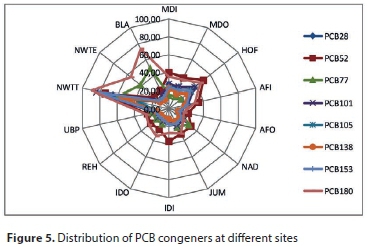
The most contaminated site was NWTT (Fig. 6 and Fig. A8, Appendix). This was attributed to the accumulation of contaminants from wastewater since the site stores wastewater before it is discharged into the river. Being a store of wastewater and having an excess of plant life as a result of eutrophication, this site (NWTT) may contain more organic carbon than other sites. This may allow for partitioning of more PCBs and may be the reason for the high concentrations found at this site. A study of fate and persistence of PCBs in soil revealed that their persistence was greater in soil with higher organic carbon content (Ayris and Harrad, 1999).

 

 

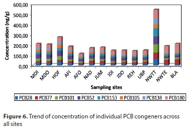
Comparison of levels of PCBs and OCPs in soil from various locations globally

The levels of PCBs detected in the present study were compared to the levels of PCBs detected in various locations around the world (Table 5). The total PCB concentration ranged from 112.79 to 542.95 ng/g, with mean of 203.73 ng/g) (Table 4). The PCB concentrations detected were lower than the results obtained by Yuan and co-workers who found total PCB concentrations in topsoils of Beijing in China ranging from 47.04 to 3 883.77 ng/g, with a mean of 679.62 ng/g (Yuan et al., 2014). Levels of PCBs in eastern Romania were determined by Dragan and co-workers who found this to range between 34 and 1 132 ng/g, with a mean of 278 ng/g (Dragan et al., 2006). The total concentrations of OCPs in topsoil of Beijing in China were found to vary from 2.38 to 933.12 ng/g, with a mean of 68.76 ng/g (Yuan et al., 2014). Table 5 summarizes the results obtained from different regions of the globe. The results obtained in this study were far below those reported by Yuan and co-workers in the top-soil of a topical urban area in Beijing, China, where the levels of OCPs ranged from 2.4 to 3 883.8 ng/g (Yuan et al., 2014), as well as those detected in South East Romanian soil (58-1662 ng/g) (Ene et al., 2012) and those detected at Patagonia in Argentinian soil (38 100-46 500 ng/g) (Gonzaleza et al., 2010). However, the Umgeni River OCP levels were higher than the levels investigated in the Chao River soil in China (0.8145-16.8524 ng/g) (Yu et al., 2014).

Being ubiquitous, the organochlorine pesticides occur everywhere in any environmental compartment in different parts of the globe. Table 6 shows the comparison of the results of the present study with those of other investigations carried out worldwide.

 

CONCLUSION

In this study, assessment of the levels and distribution of OCPs and PCBs in soil collected from the banks of the Umgeni River was carried out. All the contaminants investigated were detected at all sites. The distribution of OCPs and PCBs in the soil from the banks of the Umgeni River was ubiquitous because of different potential sources, such as agricultural runoff, industries, wastewater treatment plants and non-point sources. Considering the levels of OCPs and PCBs detected in this study, the bank soil from the Umgeni River is contaminated, which may leach into the river. Therefore, serious measures must be taken by the local government to reduce the contamination effects of the river water and protect the environment. This was the first study on the presence of organic pollutants in the soil of the Umgeni River which has added to the present limited knowledge of their environmental distribution in bank river soils from KwaZulu-Natal in South Africa.

 

ACKNOWLEDGEMENTS

The authors are grateful to the University of KwaZulu-Natal, Water Research Commission (WRC) of South Africa and Government of Rwanda, through Rwanda Education Board (REB), for financial support. The constructive advice of Dr F Agunbiade is appreciated.

 

REFERENCES

AGAPKINA GI, EFIMENKO ES, BRODSKIY ES, SHELEPCHIKOV AA and FESHIN DB (2012) Priority organic pollutants in soil of arboretum in botanical garden of Lomonosov MSU report 1. Peculiarities of vertical distribution of polychlorinated biphenyls in urbanozem profile. Vestnik Moskovskogo Univ. 17 42-49.         [ Links ]

AIGNER EJ, LEON AD and FALCONER RL (1998) Concentrations and enantiomeric ratios of organochlorine pesticides in soils from the U.S. corn belt. Environ. Sci. Technol. 32 1162-1168. https://doi.org/10.1021/es970750h        [ Links ]

AYRIS S and HARRAD S (1999) The fate and persistence of polychlorinated biphenyls in soil. J. Environ. Monit. 1 395-401. https://doi.org/10.1039/a903017d        [ Links ]

BARRIADA-PEREIRA M, GONZALEZ-CASTRO MJ, MUNIATEGUI-LORENZO S, LOPEZ-MAHIA P, PRADA-RODRIGUEZ D and FERNANDEZ-FERNANDEZ E (2005) Organochlorine pesticides accumulation and degradation products in vegetation samples of a contaminated area in Galicia (NW Spain). Chemosphere 58 1571-1578. https://doi.org/10.1016/j.chemosphere.2004.10.016        [ Links ]

BARRIE LA, GREGOR D, HARGRAVE B, LAKE R, MUIR D, SHEARER R, TRACEY B and BIDLEMAN T (1992) Arctic contaminants: sources, occurrences and pathways. Sci. Total Environ. 122 1-74. https://doi.org/10.1016/0048-9697(92)90245-N        [ Links ]

BIDLEMAN TF, FALCONER RL and WALLA MD (1995) Toxaphene and other organochlorine compounds in air and water at Resolute Bay, N.W.T., Canada. Sci. Total Environ. 160 & 161 55-63. https://doi.org/10.1016/0048-9697(95)04344-Z        [ Links ]

BOUWMAN H, COOPPAN RM, BECKER PJ and NGXONGO S (1991) Malaria control and levels of DDT in serum of two populations in KwaZulu-Natal. J. Toxicol. Environ. Health 33 141-155. https://doi.org/10.1080/15287399109531514        [ Links ]

BREIVIK K, GIOIA R, CHAKLABORTY P, ZHANG G and JONES KC (2011) Are reductions in industrial organic contaminants emmissions in rich countries achieved partly by export of toxic wastes? Environ. Sci. Technol. 45 9154-9160. https://doi.org/10.1021/es202320c        [ Links ]

CONCHA-GRANA E, TURNES-CAROU MI, MUNIATEGUI-LORENZO S, LOPEZ-MAHIA P, PRADA-RODRIGUEZ D and FERNANDEZ-FERNANDEZ E (2006) Evaluation of HCH isomers and metabolites in soils, leachates, river water and sediments of a highly contaminated area. Chemosphere 64 588-595. https://doi.org/10.1016/j.chemosphere.2005.11.011        [ Links ]

DE VOOGT P, WELLS DE, REUTERGRDH L and BRINKMAN UAT (1990) Biological activity, determination and occurrence of planar, mono-ortho and di-ortho PCBs. Int. J. Environ. Anal. Chem. 40 1-46. https://doi.org/10.1080/03067319008030516        [ Links ]

DIMITROVA A, STOYANOVA Y and TACHEV A (2013) Distribution and risk assessment of polychlorinated biphenyls (PCBs) in urban soils of Sofia City, Bulgaria. In: Duarte JA, Kibler MR and Hefferlin R (eds) Recent Advances in Chemical Engineering, Biochemistry and Computational Chemistry. ISBN:978-960-474-342-1. 48-54.         [ Links ]

DIMOND JB and OWEN RB (1996) Long-term residue of DDT compounds in forest soils in Maine. Environ. Pollut. 92 227-230. https://doi.org/10.1016/0269-7491(95)00059-3        [ Links ]

DOINA T, SIMONA CM, JANA B, JANA K and ADRIAN C (2013) Organochlorine pesticides in soil, moss and tree-bark from North-Eastern Romania. Sci. Total Environ. 456-457 317-324. https://doi.org/10.1016/j.scitotenv.2013.03.103        [ Links ]

DRAGAN D, CUCU-MAN S, DIRTU AC, MOCANU R, VAECK LV and COVACI A (2006) Occurrence of organochlorine pesticides and polychlorinated biphenyls in soils and sediments from Eastern Romania. Int. J. Environ. Anal. Chem. 86 833-842. https://doi.org/10.1080/03067310600665571        [ Links ]

ENE A, BOGDEVICHB O and SIONA A (2012) Levels and distribution of organochlorine pesticides (OCPs) and polycyclic aromatic hydrocarbons (PAHs) in topsoils from SE Romania. Sci. Total Environ. 439 76-86. https://doi.org/10.1016/j.scitotenv.2012.09.004        [ Links ]

FALANDYSZ J, BRUDNOWSKA B, KAWANO and WAKIMOTO T (2001) Polychlorinated biphenyls and organochlorine pesticides in soils from the southern part of Poland. Arch. Environ. Contam. Toxicol. 40 173-178. https://doi.org/10.1007/s002440010160        [ Links ]

GAO Y, WANG Y and ZHOU Q (2015) Distribution and temporal variation of PCBs and PAHs in soils and sediments from an e-waste dismantling site in china. Environ. Earth Sci. 74 2925-2935. https://doi.org/10.1007/s12665-015-4320-z        [ Links ]

GONG ZM, TAO S, XU FL, DAWSON R, LIU WX, CUI YH, CAO J, WANG XJ, SHEN WR, ZHANG WJ, QING BP and SUN R (2004) Level and distribution of DDT in surface soils from Tianjing, China. Chemosphere 54 1247-1253. https://doi.org/10.1016/j.chemosphere.2003.10.021        [ Links ]

GONZALEZA M, MIGLIORANZA KSB, AIZPUNA JE, ISLA FI and PENAB A (2010) Assessing pesticide leaching and desorption in soils with different agricultural activities from Argentina (Pampa and Patagonia). Chemosphere 81 351-358. https://doi.org/10.1016/j.chemosphere.2010.07.021        [ Links ]

HARNER T, BIDLEMAN TF, JANTUNEN LMM and MACKAY D (2001) Soil-air exchange model of persistent pesticides in the United States cotton belt. Environ. Toxicol. Chem. 20 1612-1621. https://doi.org/10.1002/etc.5620200728        [ Links ]

HARRY BM, LYNN SW and JUDITH AS (2008) Alternative approches to collecting and interpreting matrix spike data. 27^th Annual EPA Conference on Managing Environmental Quality Systems. URL: http://www.epa.gov/QUALITY/qs-2008/alternative.pdf (Accessed 12 June 2014).         [ Links ]

JONES KC and DE VOOGT P (1999) Persistent organic pollutants (POPs): state of the science. Environ. Pollut. 100 209-221. https://doi.org/10.1016/S0269-7491(99)00098-6        [ Links ]

LI BG, CAO J, LIU WX, SHEN WR, WANG XJ and TAO S (2006) Geostatistical analysis and kriging of hexachlorocyclohexane residues in topsoil from Tianjin, China. Environ. Pollut. 142 567-575. https://doi.org/10.1016/j.envpol.2005.10.039        [ Links ]

LI Y and MACDONALD R (2005) Sources and pathways of selected organochlorine pesticides to the Arctic and the effect of pathway divergence on HCH trends in biota: A review. Sci. Total Environ. 342 87−106. https://doi.org/10.1016/j.scitotenv.2004.12.027        [ Links ]

LI YF (1999) Global technical hexachlorocyclohexane usage and its contamination consequences in the environment: from 1948 to 1997. Sci. Total Environ. 232 121-158. https://doi.org/10.1016/S0048-9697(99)00114-X        [ Links ]

LI Y, SCHOLTZ MT and MCMILLAN A (1996) Global HCH usage with longitude/latitude resolution. Environ. Sci. Technol. 30 3525-3533. https://doi.org/10.1021/es960312v        [ Links ]

LIU H, QI S, YANG D, HU Y, LI F, LIU J and XING X (2013) Soil concentrations and soil-air exchange of organochlorine pesticides along the Aba profile, east of the Tibetan Plateau, western China. Earth Sci. 7 395-405.         [ Links ]

MAHARAJ R, MTHEMBU DJ and SHARP BL (2005) Impact of DDT re-introduction on malaria transmission in KwaZulu-Natal. S. Afr. Med. J. 95 871-874        [ Links ]

MALISZEWSKA-KORDYBACH B, SMRECZAK B and KLIMKOWICZ-PAWLAS A (2014) Evaluation of status of contamination of arable soils in Poland with DDT and HCH residues; national and regional scales. Pol. J. Environ. Stud. 23 139-148.         [ Links ]

MANOHAR K, SRINIVASA RS and MOHAN KR (2014) Spatial distribution, ecological risk evaluation and potential sources of organochlorine pesticides from soils in India. Environ. Earth Sci. 74 4031. https://doi.org/10.1007/s12665-014-3189-6        [ Links ]

MEIJER SN, STEINNES E, OCKENDEN WA and JONES KC (2002) Influence of environmental variables on the spatial distribution of PCBs in Norwegian and UK soils: implications for global cycling. Environ. Sci. Technol. 36 2146-2153. https://doi.org/10.1021/es010322i        [ Links ]

MIGLIORANZA KSB, DE MORENO JEA and MORENO JV (2003) Dynamics of organochlorine pesticides in soils from a southeastern region of Argentina. Environ. Toxicol. Chem. 22 712-717. https://doi.org/10.1002/etc.5620220405        [ Links ]

NAKATA H, KAWAZOE M, ARIZONO K, ABE S, KITANO T, SHIMADA H, LI W and DING X (2002) Organochlorine pesticides and polychlorinated biphenyl residues in foodstuffs and human tissues from China: status of contamination, historical trend, and human dietary exposure. Arch. Environ. Contam. Toxicol. 43 473-480. https://doi.org/10.1007/s00244-002-1254-8        [ Links ]

NAUD Y and ROHWER ER (2012) Novel method for determing DDT in vapour and particulate phases within contaminated indoor air in a malaria area of south Africa. Anal. Chim. Acta 730 112-119. https://doi.org/10.1016/j.aca.2012.02.054        [ Links ]

OLESZEK-KUDLAK S, SHIBATA E, NAKAMURA T, Li XW, YUA YM and DONGA XD (2007) Review of the sampling and pretreatment methods for dioxins determination in solids, liquids and gases. J. Chin. Chem. Soc. 54 245-262. https://doi.org/10.1002/jccs.200700037        [ Links ]

PREDA M, LACATUSU R, MOTELICA DM, VRINCEANU N and TANASE V (2010) Adsorption of polychlorinated biphenyls by soil. Ann. Food Sci. Technol. 11 36-40.         [ Links ]

RIBES A and GRIMALT JO (2002) Temperature and organic matter dependence of the distribution of organochlorine compounds in mountain soils from the subtropical Atlantic (Teide, Tenerife Island). Environ. Sci. Technol. 36 821-827. https://doi.org/10.1021/es010272h        [ Links ]

ROLLIN HB, SANDANGER TM, HANSEN R, CHANNA K and ODLAND JO (2009) Concentration of selected persistent organic pollutants in blood from delivering women in South Africa. Sci. Total Environ. 408 146-152.         [ Links ]

ROTHER HA and JACOBS R (2008). Pesticide health risk for South African emerging farmers. Surplus People Project (SPP), Cape Town. URL: http://www.spp.org.za/booklets/pesticide_booklet.pdf (Accessed 26 June 2014).         [ Links ]

SADASIVAIAH S, TOZAN Y and BREMAN JG (2007) Dichlorodiphenyltrichloroethane (DDT) for indoor spraying in Africa: How can it be used for malaria control? Am J. Trop. Med. Hyg. 77 249-264. https://doi.org/10.4269/ajtmh.2007.77.249        [ Links ]

SHRIVASTAVA A and GUPTA VB (2011) Method for the determination of limit of detection and limit of quantitation of the analytical methods. Chron. Young Sci. 2 21-25. https://doi.org/10.4103/2229-5186.79345        [ Links ]

SULTANA J, SYED JH, MAHMOOD A, ALI U, ABDUR REHMAN MY, MALIK RN, LI J and ZHANG G (2014) Investigation of organochlorine pesticides from the Indus Basin, Pakistan: Sources, air-soil exchangefluxes and risk assessment. Sci. Total Environ. 497-498 113-122. https://doi.org/10.1016/j.scitotenv.2014.07.066        [ Links ]

THOMPSON AL, DARWISH SW, IKENAKA Y, NAKAYAMA MMS, MIZUKAWA H and ISHIZUKA M (2017) Organochlorine pesticide contamination of foods in Africa: incidence and public health significance. J. Vet. Med. Sci. 79 751-764. https://doi.org/10.1292/jvms.16-0214        [ Links ]

USEPA (United States Environmental Protection Agency) (1996) Method 3540C: soxhlet extraction. URL: http://www.epa.gov/osw/hazard/testmethods/sw846/pdfs/3540c.pdf [Accessed 10 March 2014). USEPA, Washington DC.         [ Links ]

USEPA (United States Environmental Protection Agency) (2007) Method 3620: Florisil cleanup. URL: http://www.epa.gov/osw/hazard/testmethods/sw846/pdfs/3620c.pdf (Accessed 10 March 2014). USEPA, Washington DC.         [ Links ]

USEPA (United States Environmental Protection Agency) (2007b) Method 1699: Pesticides in water, soil, sediment, biosolids, and tissue by HRGC/HRMS (EPA-821-R-08-001). URL: https://www.epa.gov/sites/production/files/2015-10/documents/method_1699_2007.pdf (Accessed 31 October 2014). USEPA, Washington DC.         [ Links ]

USEPA (United States Environmental Protection Agency) (2008) Method 1668B: Chlorinated biphenyl congeners in water, soil, sediment, biosolids, and tissue by HRGC/HRMS. Quantitative determination. USEPA, Washington DC.         [ Links ]

USEPA (United States Environmental Protection Agency) (2009) Technical factsheet on: Endrin. URL: http://www.epa.gov/ogwdw/pdfs/factsheets/soc/tech/endrin.pdf (Accessed 12 April 2015). USEPA, Washington DC.         [ Links ]

VAN DYK JC, BOUWMAN H, BARNHOORN IEJ and BORNMAN M (2010) DDT contamination from indoor residual spraying for malaria control. Sci. Total Environ. 408 2745-2752. https://doi.org/10.1016/j.scitotenv.2010.03.002        [ Links ]

VANE CH, KIM AW, BERIRO DJ, CAVE MR, NIGHTS K, MOSS-HAYES V, NATHANAIl CP (2014). Polycyclic aromatic hydrocarbons (PAH) and polychlorinated biphenyls (PCB) in urban soils of Greater London, UK. Appl. Geochem. 51 303-314. https://doi.org/10.1016/j.apgeochem.2014.09.013        [ Links ]

VESNA M, DANIJELA B, ANTE B, TOMISLAV Z,) (2006) Distribution of polychlorinated biphenyls (PCBs) in surface sediments from the Middle and South Adriatic coastal waters. Fresen. Environ. Bull. 15 997-1002.         [ Links ]

VOLDNER EC, LI, YF (1995) Global usage of selected persistent organochlorines. Sci. Total Environ.160 201-210. https://doi.org/10.1016/0048-9697(95)04357-7        [ Links ]

WANG Y, LUO CL, LI G, YIN H, LI XD, ZHANG G (2011) Characterisation and risk assessment of polychlorinated biphenyls in soils and vegetations near an electronic waste recycling site, South China. Chemosphere 85 344-350. https://doi.org/10.1016/j.chemosphere.2011.06.096        [ Links ]

WANG F, JIANG X, BIAN YR, YAO FX, GAO HJ, YU GF, MUNCH JC, SCCHROLL R (2007) Organochlorine pesticides in soils under different land usage in the Taihu Lake region, China. J. Environ. Sci. 19 584-590. https://doi.org/10.1016/S1001-0742(07)60097-7        [ Links ]

WHO (2010) World malaria report, World Health Organization. URL: http://www.who.int/malaria/publications/country-profiles/profile_zaf_en.pdf (Accessed 12 April 2015).         [ Links ]

WILCKE W, KRAUSS M, SAFRONOV G, FOKIN AD and KAUPENJOHANN M (2006) Polychlorinated biphenls (PCBs) in soils of the Moscow region: concentrations and small-scale distribution along an urban-rural transect. Environ. Pollut. 141 327-335. https://doi.org/10.1016/j.envpol.2005.08.038        [ Links ]

WILD SR and JONES KC (1995) Polynuclear aromatic-hydrocarbons in the United-Kingdom environment - a preliminary source inventory and budget. Environ. Pollut. 88 91-108. https://doi.org/10.1016/0269-7491(95)91052-M        [ Links ]

WONG MH, WU SC, DENG WJ, YU XZ, LUO Q and LEUNG AOW (2007) Export of toxic chemicals-a review of the case of uncontrolled electronic-waste recycling. Environ. Pollut. 149 131-140. https://doi.org/10.1016/j.envpol.2007.01.044        [ Links ]

YU Y, LI Y, SHEN Z, YANG Z, MO L, KONG Y and LOU I (2014) Occurrence and possible sources of organochlorine pesticides (OCPs) and polychlorinated biphenyls (PCBs) along the Chao River, China. Chemosphere 114 136-143. https://doi.org/10.1016/j.chemosphere.2014.03.095        [ Links ]

YUAN GL, WU HZ, FU S, HAN P and LANG XX (2014) Persistent organic pollutants (POPs) in the topsoil of typical urban renewal area in Beijing, China: Status, sources and potential risk. J. Geochem. Explor. 138 94-103. https://doi.org/10.1071/EG13066        [ Links ]

ZHONGHUA Z, HAIAO Z, JINGLU W and LU Z (2013) Organochlorine pesticide (OCP) residues in mountain soils from Tajikistan. Environ. Sci Process Imp. 15 608-616. https://doi.org/10.1039/c2em30849e        [ Links ]

ZHU ZC, CHEN SJ, ZHENG J, TIAN M, FENG AH, LUO XJ and MAI BX (2014) Occurrence of brominated flame retardants (BFRs), organochlorine pesticides (OCPs), and polychlorinated biphenyls (PCBs) in agricultural soils in a BFR-manufacturing region of North China. Sci. Total Environ. 481 47-54. https://doi.org/10.1016/j.scitotenv.2014.02.023        [ Links ]

 

 

Received 19 December 2018
Accepted in revised form 23 September 2019

 

 

* Corresponding author, email: Moodleyb3@ukzn.ac.za

 

 

 

 

 

 

 

 

 

 

 

 

 

 

 

 

^rND^sAGAPKINA^nGI^rND^sEFIMENKO^nES^rND^sBRODSKIY^nES^rND^sSHELEPCHIKOV^nAA^rND^sFESHIN^nDB^rND^sAIGNER^nEJ^rND^sLEON^nAD^rND^sFALCONER^nRL^rND^sAYRIS^nS^rND^sHARRAD^nS^rND^sBARRIADA-PEREIRA^nM^rND^sGONZALEZ-CASTRO^nMJ^rND^sMUNIATEGUI-LORENZO^nS^rND^sLOPEZ-MAHIA^nP^rND^sPRADA-RODRIGUEZ^nD^rND^sFERNANDEZ-FERNANDEZ^nE^rND^sBARRIE^nLA^rND^sGREGOR^nD^rND^sHARGRAVE^nB^rND^sLAKE^nR^rND^sMUIR^nD^rND^sSHEARER^nR^rND^sTRACEY^nB^rND^sBIDLEMAN^nT^rND^sBIDLEMAN^nTF^rND^sFALCONER^nRL^rND^sWALLA^nMD^rND^sBOUWMAN^nH^rND^sCOOPPAN^nRM^rND^sBECKER^nPJ^rND^sNGXONGO^nS^rND^sBREIVIK^nK^rND^sGIOIA^nR^rND^sCHAKLABORTY^nP^rND^sZHANG^nG^rND^sJONES^nKC^rND^sCONCHA-GRANA^nE^rND^sTURNES-CAROU^nMI^rND^sMUNIATEGUI-LORENZO^nS^rND^sLOPEZ-MAHIA^nP^rND^sPRADA-RODRIGUEZ^nD^rND^sFERNANDEZ-FERNANDEZ^nE^rND^sDE VOOGT^nP^rND^sWELLS^nDE^rND^sREUTERGRDH^nL^rND^sBRINKMAN^nUAT^rND^sDIMITROVA^nA^rND^sSTOYANOVA^nY^rND^sTACHEV^nA^rND^sDIMOND^nJB^rND^sOWEN^nRB^rND^sDOINA^nT^rND^sSIMONA^nCM^rND^sJANA^nB^rND^sJANA^nK^rND^sADRIAN^nC^rND^sDRAGAN^nD^rND^sCUCU-MAN^nS^rND^sDIRTU^nAC^rND^sMOCANU^nR^rND^sVAECK^nLV^rND^sCOVACI^nA^rND^sENE^nA^rND^sBOGDEVICHB^nO^rND^sSIONA^nA^rND^sFALANDYSZ^nJ^rND^sBRUDNOWSKA^nB^rND^sKAWANO^rND^sWAKIMOTO^nT^rND^sGAO^nY^rND^sWANG^nY^rND^sZHOU^nQ^rND^sGONG^nZM^rND^sTAO^nS^rND^sXU^nFL^rND^sDAWSON^nR^rND^sLIU^nWX^rND^sCUI^nYH^rND^sCAO^nJ^rND^sWANG^nXJ^rND^sSHEN^nWR^rND^sZHANG^nWJ^rND^sQING^nBP^rND^sSUN^nR^rND^sGONZALEZA^nM^rND^sMIGLIORANZA^nKSB^rND^sAIZPUNA^nJE^rND^sISLA^nFI^rND^sPENAB^nA^rND^sHARNER^nT^rND^sBIDLEMAN^nTF^rND^sJANTUNEN^nLMM^rND^sMACKAY^nD^rND^sJONES^nKC^rND^sDE VOOGT^nP^rND^sLI^nBG^rND^sCAO^nJ^rND^sLIU^nWX^rND^sSHEN^nWR^rND^sWANG^nXJ^rND^sTAO^nS^rND^sLI^nY^rND^sMACDONALD^nR^rND^sLI^nYF^rND^sLI^nY^rND^sSCHOLTZ^nMT^rND^sMCMILLAN^nA^rND^sLIU^nH^rND^sQI^nS^rND^sYANG^nD^rND^sHU^nY^rND^sLI^nF^rND^sLIU^nJ^rND^sXING^nX^rND^sMAHARAJ^nR^rND^sMTHEMBU^nDJ^rND^sSHARP^nBL^rND^sMALISZEWSKA-KORDYBACH^nB^rND^sSMRECZAK^nB^rND^sKLIMKOWICZ-PAWLAS^nA^rND^sMANOHAR^nK^rND^sSRINIVASA^nRS^rND^sMOHAN^nKR^rND^sMEIJER^nSN^rND^sSTEINNES^nE^rND^sOCKENDEN^nWA^rND^sJONES^nKC^rND^sMIGLIORANZA^nKSB^rND^sDE MORENO^nJEA^rND^sMORENO^nJV^rND^sNAKATA^nH^rND^sKAWAZOE^nM^rND^sARIZONO^nK^rND^sABE^nS^rND^sKITANO^nT^rND^sSHIMADA^nH^rND^sLI^nW^rND^sDING^nX^rND^sNAUD^nY^rND^sROHWER^nER^rND^sOLESZEK-KUDLAK^nS^rND^sSHIBATA^nE^rND^sNAKAMURA^nT^rND^sLi^nXW^rND^sYUA^nYM^rND^sDONGA^nXD^rND^sPREDA^nM^rND^sLACATUSU^nR^rND^sMOTELICA^nDM^rND^sVRINCEANU^nN^rND^sTANASE^nV^rND^sRIBES^nA^rND^sGRIMALT^nJO^rND^sROLLIN^nHB^rND^sSANDANGER^nTM^rND^sHANSEN^nR^rND^sCHANNA^nK^rND^sODLAND^nJO^rND^sSADASIVAIAH^nS^rND^sTOZAN^nY^rND^sBREMAN^nJG^rND^sSHRIVASTAVA^nA^rND^sGUPTA^nVB^rND^sSULTANA^nJ^rND^sSYED^nJH^rND^sMAHMOOD^nA^rND^sALI^nU^rND^sABDUR REHMAN^nMY^rND^sMALIK^nRN^rND^sLI^nJ^rND^sZHANG^nG^rND^sTHOMPSON^nAL^rND^sDARWISH^nSW^rND^sIKENAKA^nY^rND^sNAKAYAMA^nMMS^rND^sMIZUKAWA^nH^rND^sISHIZUKA^nM^rND^sVAN DYK^nJC^rND^sBOUWMAN^nH^rND^sBARNHOORN^nIEJ^rND^sBORNMAN^nM^rND^sVANE^nCH^rND^sKIM^nAW^rND^sBERIRO^nDJ^rND^sCAVE^nMR^rND^sNIGHTS^nK^rND^sMOSS-HAYES^nV^rND^sNATHANAIl^nCP^rND^sVESNA^nM^rND^sDANIJELA^nB^rND^sANTE^nB^rND^sTOMISLAV^nZ^rND^sVOLDNER^nEC^rND^sLI^nYF^rND^sWANG^nY^rND^sLUO^nCL^rND^sLI^nG^rND^sYIN^nH^rND^sLI^nXD^rND^sZHANG^nG^rND^sWANG^nF^rND^sJIANG^nX^rND^sBIAN^nYR^rND^sYAO^nFX^rND^sGAO^nHJ^rND^sYU^nGF^rND^sMUNCH^nJC^rND^sSCCHROLL^nR^rND^sWILCKE^nW^rND^sKRAUSS^nM^rND^sSAFRONOV^nG^rND^sFOKIN^nAD^rND^sKAUPENJOHANN^nM^rND^sWILD^nSR^rND^sJONES^nKC^rND^sWONG^nMH^rND^sWU^nSC^rND^sDENG^nWJ^rND^sYU^nXZ^rND^sLUO^nQ^rND^sLEUNG^nAOW^rND^sYU^nY^rND^sLI^nY^rND^sSHEN^nZ^rND^sYANG^nZ^rND^sMO^nL^rND^sKONG^nY^rND^sLOU^nI^rND^sYUAN^nGL^rND^sWU^nHZ^rND^sFU^nS^rND^sHAN^nP^rND^sLANG^nXX^rND^sZHONGHUA^nZ^rND^sHAIAO^nZ^rND^sJINGLU^nW^rND^sLU^nZ^rND^sZHU^nZC^rND^sCHEN^nSJ^rND^sZHENG^nJ^rND^sTIAN^nM^rND^sFENG^nAH^rND^sLUO^nXJ^rND^sMAI^nBX^rND^1A01^nDM^sJacklin^rND^1A02^nIC^sBrink^rND^1A01^nJ^sde Waal^rND^1A01^nDM^sJacklin^rND^1A02^nIC^sBrink^rND^1A01^nJ^sde Waal^rND^1A01^nDM^sJacklin^rND^1A02^nIC^sBrink^rND^1A01^nJ^sde Waal

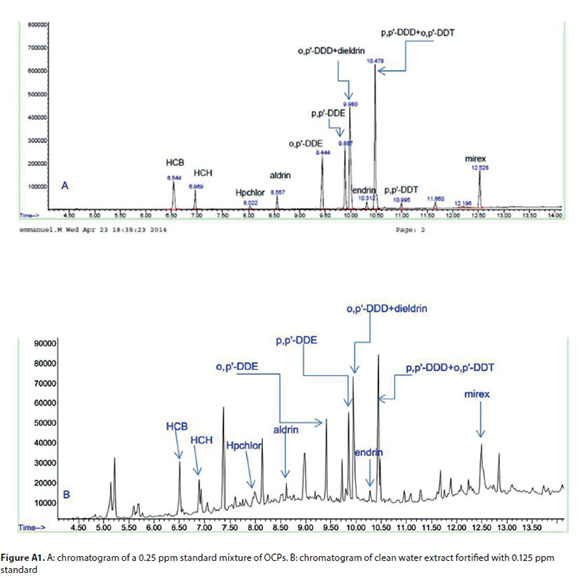
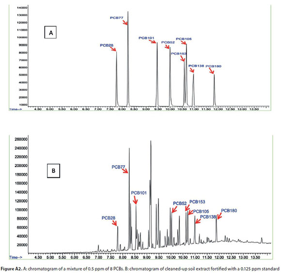
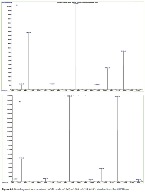
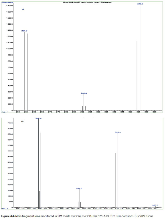
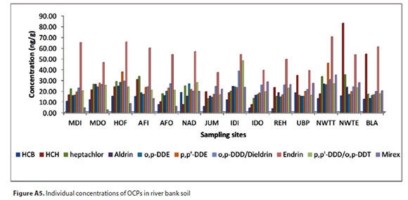
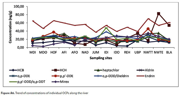
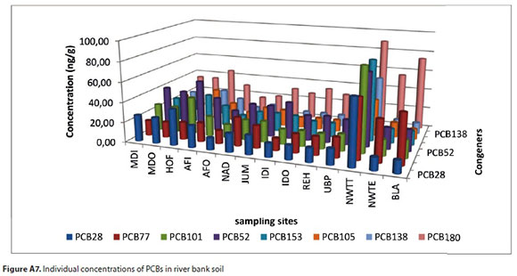
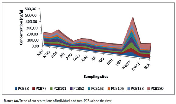
RESEARCH PAPERS

 

Laboratory method design for investigating the phytoremediation of polluted water

 

 

DM Jacklin^I; IC Brink^II; J de Waal^{I, *}

^IDepartment of Geography and Environmental Studies, Stellenbosch University, Private Bag X1, Matieland 7602, South Africa
^IIDepartment of Water and Environmental Engineering, Stellenbosch University, Private Bag X1, Matieland 7602, South Africa

 

 

---

ABSTRACT

The performance of plants to remove, remediate or immobilise environmental contaminants in a growth matrix through natural biological, chemical or physical activities was studied in a laboratory phytoremediation system. This study aimed to develop a novel phytoremediation system capable of investigating the remediation of agricultural pollutants by individual and multiple plant species. The designed system analysed community phytoremediation by uniquely implementing multiple plant species within the same growth silo, with indigenous and alien assemblages compared to establish community performance, highlighting the importance of biodiversity in plant assemblages. The constructed system successfully analysed the phytoremediatory capabilities of plant species within the critically endangered Renosterveld vegetation type, with unvegetated soil controls included to illustrate the pollutant removal efficiency of plants only. Growth silos were constructed from PVC piping and irrigated with drippers from a submersible pump. Eighteen different plant species were included in the experiment, i.e., 14 indigenous species, 3 invasive alien plant (IAP) species, and Palmiet. Five agricultural pollutant parameters were analysed, i.e., for fertilizers NH₃-N, NO₃⁻-N and PO₄³⁻-P and for herbicide contamination using two glyphosate concentrations. The growth silos and unvegetated soil control were irrigated using a pollutant-municipal water solution at 3-day intervals. The multiple plants per silo design approach seeks to contribute to the limited literature pertaining heterogeneity importance, by comparing the pollutant removal performance of plant assemblages. Community comparison further investigated the biofilter implementation potential of indigenous South African plants as an alternative to their more invasive alien counterparts, adding to the knowledge base of plant-based phytoremediation by indigenous South African plant species. The laboratory phytoremediation system successfully measured the agricultural pollutant removal performance of individual plants and vegetative communities, with soil remediation influence acknowledged. The proposed system is a simple and inexpensive method for obtaining the plant-based biofiltration efficiency of individual and multiple plant species.

Keywords: experimental design, phytoremediation, water quality, bioremediation

---

 

 

INTRODUCTION

Globally, terrestrial surface and groundwaters are affected by pollution from a range of industrial and agricultural activities (Schoumans et al., 2014). In particular, fertilizers and pesticides, derived from various agricultural practices, lead to the degradation of both surface and groundwater (Barcelo, 1997; Donoso et al., 1999; Lam et al., 2010). Diffuse water pollution from agricultural applications carry an immense cost to society, including environmental and ecosystem damage, loss of aquaculture and fisheries income and increased treatment costs for drinking water (Norse et al., 2001; Norse, 2005; Smith and Siciliano, 2015). Nitrogen (N) and phosphorus (P) fertilizers, and glyphosate-based (C₃H₈NO₅P) herbicides, can cause nutrient loading and widespread water quality degradation to both surface and groundwater (Schachtschneider et al., 2010; Hashemi et al., 2016). However, vegetation buffers between agricultural fields and watercourses can potentially slow the migration of chemicals, thus limiting agricultural pollutants into adjacent waterways (Campbell, 1999; Beltrano et al., 2013). Due to the hazardous effects of agricultural pollutants on the environment, specifically non-point source aquatic ecosystem pollution, techniques to reduce nutrient and herbicide discharge must be developed (Tesfamariam et al., 2009; Schoumans et al., 2014).

In developing countries phytoremediation has become a technology of choice for remediation projects, due to cost-effectiveness and implementation ease (Terry and Banuelos, 1999). The technique additionally takes into account the probable end-use of the site once it has been remediated (Pilon-Smits, 2005). Conventional approaches to remediation often produce infertile soil by destroying the microenvironment (Kennen and Kirkwood, 2015). Additionally, knowledge regarding the phytoremediatory capabilities of individual plant species is limited. Since plants and soils respond differently when exposed to polluted water, it is essential to determine the independent remediation efficiencies of these media. For effective phytoremediation, the implemented system needs to be capable of remediating pollutants without displaying ecosystem invasive properties. It is for this reason that the phytoremediatory capabilities of individual plant species and a vegetative community as a whole need to be studied.

The purpose of this paper is to demonstrate the design and construction of a laboratory phytoremediation system, capable of establishing the performance of individual plant species and vegetative communities, by investigating agricultural pollutant remediation. In assessing the remediation performance of multiple plants per growth silo, the important role of biodiversity in vegetative assemblages is highlighted. The efficacy of the proposed laboratory method design is tested by comparing the pollutant extraction capabilities of individual, multiple-indigenous and alien wetland plant species commonly used for phytoremediation.

 

MATERIALS AND METHODS

Experimental design

To evaluate the pollutant extraction capabilities of plant species, the system was required to integrate 5 influent pollutants across multiple growth silos whilst guaranteeing uniform standardized influent irrigation throughout. Growth silos were constructed from polyvinyl chloride (PVC) piping, each containing a threaded slit drainage pipe that protruded from the sealed base of each silo - enabling effluent collection into sampling containers directly below. Silos for individual plants and larger growth silos for multiple species (indigenous and alien) within a singular silo were constructed from PVC, to test the overall contribution of phytoremediation (Fig. 1). The larger silos accommodated 4 plant species within each silo. Voids were cut along the length of the silos for the establishment of plants at different intervals. At each void a plant species was introduced. The quantity per plant species introduced depended on the surface cover associated with that species, for instance, quantity of grasses to be introduced was greater than the quantity of sedges. For each growing compartment (void) a roof-like structure was inserted, ensuring soil stability and preventing collapsed media and pollutants cascading onto and potentially harming the plants.

An equivalent growth medium volume between different silo sizes ensured that the effect of degradation and adsorption by soil was consistent. It is important to acknowledge the remediation effect of soil media within the different silo sizes, thus soil controls associated with the different silo sizes were included.

Soil growth volume calculation

For the individual plant per silo experiment, the silo dimensions were selected to represent a growth volume (V) capable of supporting rhizosphere processes and plant root growth. Considering that only a portion of the silo is used as growth medium and the rest as a layer of natural filtration, the selected growth medium height for individual species per silo was 30 cm (Fig. 2).

The selected soil growth volume for all plants was standardized at 2 548.46 cm³ (Fig. 2). Growth volume for each plant species was consistent throughout. The soil control volume of the multiple plant species silo combined the soil growth volume of the individual plant species per silo, adapted to represent a combination of four species. As voids were created to allow for efficient plant growth, the growth volumes were adjusted to accommodate the areas lost by the voids.

Drainage layers

Paired drainage layers comprising of coarse sand and gravel were added below the soil growth, to cover the drainage pipe. These drainage layers prevented sedimentation within the slits of the drainage pipe, preventing clogging of the effluent runoff. The thickness of the drainage layers was comparable with previous urban drainage studies (Bratieres et al., 2008; Read et al., 2008; Milandri et al., 2012)Australia, to test the performance of stormwater biofilters for the removal of sediment, nitrogen and phosphorus. The aim of the study was to provide guidance on the optimal design for reliable treatment performance. A variety of factors were tested, using 125 large columns: plant species, filter media, filter depth, filter area and pollutant inflow concentration. The results demonstrate that vegetation selection is critical to performance for nitrogen removal (e.g. Carex appressa and Melaleuca ericifolia performed significantly better than other tested species.

Soil utilized as growth medium

The soil growth medium was selected to reflect the natural conditions for plant root growth and pollutant adsorption. The use of the soil type which the plants under study are naturally accustomed to alleviates stress during plant extraction and transplantation. For similar studies it is recommended that soil be included which is associated with the plant species under study, as rhizosphere-condition familiarity would minimise the acclimatisation period (Bunt, 2012).

Irrigation

An automated irrigation system was installed to ensure a consistent irrigation regime with frequency of 72 h. The system contained three submersible pumps, one for each of the three treatments (fertilizer, herbicide and municipal control), submersed within their respective storage containers (Fig. 3). The capacity of each container was 45 L; with each container fitted with an external clear pipe marked to indicate the volume of the solution within. The municipal control container was fitted to a municipal tap to refill the water volume as the submersible pump transported solution to the system. The capacity within the container was controlled by a domestic toilet flow inlet control valve connected to a float ball, to ensure a constant water level. Each submersible pump transferred the water from their respective storage containers using 15 mm irrigation pipes attached to 35 treatment silos via drippers; each pipe was fitted with an Emjay filter to remove any material that may impede the flow.

Added storage tanks were constructed for the herbicide and fertilizer containers. Two 70 L storage tanks were included in the study to increase the mixed herbicide and fertilizer solution capacities. The tanks were placed above the experimental set-up on scaffolding, to allow transport of fluid to the 45 L containers below, containing the submersible pumps, by gravitational flow. The solution was transported to the submersible pump containers by 15 mm irrigation lines, controlled with internal valves, with the ability to impede the flow when maintenance on the submersible pump containers was required.

The capacity of the submersible pump containers was controlled by attaching the irrigation inflow, from the storage tanks above to a domestic toilet flow inlet control valve. The valves were connected to float balls. This ensured consistent irrigation of solution volume into the growth silos. Drippers of dissimilar irrigation rates were used for the different silo sizes, 870 mL/h and 2 070 mL/h for the smaller individual plant species silos and the larger multiple plant species silos, respectively.

Treatments consisted of municipal tap water (as the control), a fertilizer solution and a herbicide solution. The solutions were mixed prior to each treatment cycle. Each container housed an additional submersible pump, to prevent stagnation and ensure complete dispersion of nutrients and chemicals. After transplantation, the plants received municipal tap water for 6 months, this period allowed the plants to acclimatize to their new growing conditions. The process was mitigated by establishing similar environmental growing conditions, with the utilization of soil excavated from the selected field study site. The duration of the acclimatization period granted the species sufficient time to develop into stronger, more mature plants and, if any adverse impacts resulting from plant transplantation and translocation were experienced, time to recuperate.

Lighting

An indoor laboratory phytoremediation system is prone to irregular natural light, limiting uniform plant growth, thus artificial lighting was provided to produce a uniform distribution. The lighting was distributed by fluorescent tubes via Osram Biolux lamps due to their wavelength distribution comparable to sunlight (Osram, 2018). Eight 58W Biolux tubes were mounted throughout the system, placed at specific locations to ensure uniform light distribution. The fluorescent lights were controlled by a mechanical timer, switching the lights on and off according to a programmable schedule. The timer was programmed to display light between 05:30 and 20:00, to reflect natural growing conditions.

Plants for phytoremediation

Plant species vary with regard to their pollutant removal abilities, with the most effective plant species characterised by long roots, deep root depth, and heavy root mass (Read et al., 2010). The introduction of certain plant species for phyto-extraction may, however, pose a set of alien invasive problems, necessitating investigation into the removal efficiencies of plant species indigenous to contaminated areas (Schachtschneider et al., 2010; Leguizamo et al., 2017). For this reason, indigenous South African plant species were included for plant-based biofilter investigation. Various phytotechnologies utilize different plant properties and typically implement different plant species for each scenario. Properties that have been accepted as advantageous to phytoremediation are: fast growing, high biomass, competitive and high tolerance to pollution (Pilon-Smits, 2005).

The pollutant removal efficiency of indigenous plant species and invasive alien plant (IAP) and Palmiet species (commonly used in phytoremediation) were investigated and compared. A sample of indigenous plants displaying non-invasive properties, and being potentially capable of remediating pollutants with either matching or superior efficacy to the IAP, and Palmiet species are tested. The implementation of these species as phyto-extractors, rather than their potentially invasive counterparts, benefit biodiversity conservation initiatives.

Plant collection and transplantation

The plant species were all either removed from areas where they naturally occur, from drainage canals and catchments, or sourced from nurseries in the Western Cape, South Africa. During the transplantation process, special attention was given to remove all visible foreign organic matter from the soil. This limited the contribution of any external factors during the phytoremediation process, ensuring equal conditions throughout the growth silos. Immediately following transplantation, the specimens received municipal tap water irrigation for 6 months, allowing time to mature and adjust to growing conditions. Thereafter, the plants received standardized contaminated fertilizer and herbicide water treatments. From Fig. 4, the individual plant species experiment and alien vs. indigenous community comparison experiment layout is depicted in the constructed laboratory system. Species locality was selected to minimise the effect of a dominant neighbour, creating a canopy and hindering light distribution, further inhibiting uniform growth.

Pollutants

The dosing concentrations of nitrogen (N) and phosphorus (P), viz. 46.376 mg/L and 17.391 mg/L, were selected as a result of recommendations from the Department of Agriculture, Forestry and Fisheries (DAFF) for site-specific agricultural practices affecting the watercourses under study (DAFF, 1996). Three analytical grade compounds were used to create a fertilizer mixture similar to the recommended products. In commercial fertilizers ammonia (NH₄) and nitrate (NO₃⁻) is generally the source of N with phosphate (PO₄³⁻) the source of P. N and P are represented by NH₄Cl + KNO₃ and K₂HPO₄ respectively. The concentration of the analytical grade compound is calculated from the initial 46.376 mg/L N and 17.391 mg/L P.

 

 

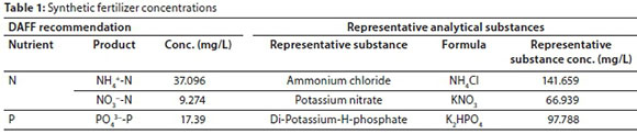
A glyphosate-based herbicide was selected to represent the agricultural herbicide pollutant on a basis of relevance, as a result of its popularity in the agricultural sector. The agricultural practices under study apply Springbok 360 SL, a product of Arysta LifeScience, prior to planting crops and after a rainfall event. Two glyphosate concentrations were selected for this study, viz. 0.7 mg/L glyphosate and 225 mg/L glyphosate; representing a non-toxic contamination to aquatic ecosystems and a worst-case scenario acute contamination, respectively.

Contamination treatment

After the initial 6-month water irrigation, the pollutant treatments commenced. The irrigation regime, every 3 days, was based on the saturation and permeability of the growth silos. A dosage of 0.653 L/3-day and 1.553 L/3-day, for the individual plant species per growth silos and multiple plant species per growth silos, respectively, was regarded as the optimum volume and rate for irrigation. Every 10 days the influent solutions were drained and replaced with a fresh mixture of pollutants, thus hindering the effect of pollutant degradation in the storage tanks.

Sampling process

Samples were collected on 5 occasions during the study. The first round of sampling was for the purpose of examining the baseline nutrient concentrations. This determined the nutrient concentrations within the growth silos prior to treatment. The baseline determination allowed for precise comparison between influent and effluent water. The percentage removal by all specimens was compared as influent concentrations were premixed to known standardized concentrations and baseline concentrations were known. Sampling intervals ensured sufficient time for previous dosage solutions to percolate through the column, ensuring influent removal analyses were not duplicated over the duration of the experiment. Sampling time correlated with the proposed irrigation schedule for agricultural activities applicable where the plants are distributed (DAFF, 2016).

Treated effluent water was collected with collection containers directly below the drainage pipes of each growth silo. Two plants per species received treatment, establishing experimental duplication and reducing outlier influence. The effluent solutions were collected in 90 mL specimen containers, with twin plant species' effluent solutions mixed post effluent collection.

Analysis

In order to evaluate the efficacy of the experiment's pollutant removal, various water quality parameters were measured throughout the experiment. These include pH, dissolved oxygen (DO), electrical conductivity (EC), nitrogen in ammonia (NH₃-N), nitrogen in nitrate (NO₃⁻-N), phosphorus in orthophosphate/soluble reactive phosphorus (PO₄³⁻-P/SRP) and glyphosate (C₃H₈NO₅P).

The pH, DO and EC were measured using the HQ440d Benchtop Multi-Parameter Meter manufactured by Hach. The NH₃-N, NO₃⁻-N and PO₄³⁻-P concentrations were measured colorimetrically using the DR3900 Benchtop Spectrophotometer and their associated TNTplus test kits. For glyphosate analysis, the acuity ultra-performance liquid chromatography (UPLC) was coupled to a Xevo Triple Quadrupole Tandem Mass Spectrometer (MS/MS) and used for high-resolution UPLC-MS/MS analysis (Waters, 2018). Glyphosate was further separated by multiple reactions monitoring (MRM) using electrospray ionisation in a positive mode.

 

RESULTS AND DISCUSSION

The experimental design allows for the comparison of chemical removal in vegetated silos and that of the soil medium control. This allows for the determination of the relative chemical absorption by both the plant and soil components. The system further indicated that there is potential to rather integrate the indigenous plant species as an alternative to their alien counterparts currently used in local and international constructed wetlands, SuDS and biofiltration systems.

In evaluating removal efficiencies (the difference between the influent and effluent concentrations), baseline concentration values need to be known. The baseline values indicate the initial nutrient content within the growth silos prior to the addition of pollutants. Without this information, one cannot deduce the removal efficiencies of the system. The initial baseline concentration of every growth silo was measured before contaminants were added to the system. Baseline concentrations were deducted from the effluent concentrations to allow for the calculation of percentage removal for each sampling round. The following equation was used:

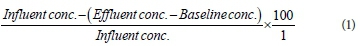
where:

Influent conc. = Influent concentration (mg/L)

Effluent conc. = Effluent concentration (mg/L)

Baseline conc. = Baseline concentration (mg/L)

The Kruskal-Wallis H-test, non-parametric ANOVA, was used for the evaluation of Renosterveld phytoremediation vs. unvegetated soil; thereafter a Student's t-test was used for the evaluation of multiple indigenous wetland plant species vs. multiple IAP species and Palmiet. Statistical analyses were executed in Python by means of the data analytical library.

Phytoremediation versus unvegetated soil

Confirming the remediation capabilities of vegetation, the concentration of pollutants removed by individual plant species was compared to the pollutants removed by the unvegetated soil silos. The percentage pollutant removal is depicted on the vertical axis as a function of time, indicating days of sampling. The initial baseline nutrient and herbicide concentrations were taken into consideration to allow for comparison between influent and effluent. Figure 5 compares the average percentage removal of all nutrients (NH₃-N, NO₃⁻-N and PO₄³⁻-P/SRP) for vegetation and the unvegetated soil control for the duration of the experiment.

 

 

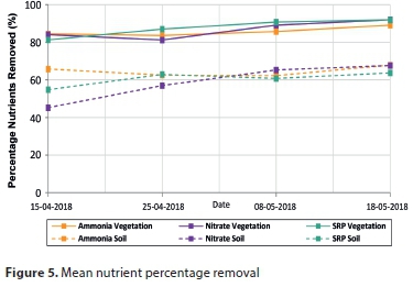
The plant species all reduced the effluent concentration of the nutrients. The percentage removal averaged 85.75%, 86.62% and 87.78% for NH₃-N, NO₃⁻-N and PO₄³⁻-P (SRP) respectively. The average percentage nutrient removal in Fig. 5 indicates that the vegetation, on average, was more effective in the removal of nutrient pollutants than was soil, attributed to the phytoremediatory capabilites of plants. There was no obvious difference between NH₃, NO₃⁻ and PO₄³⁻ remediation within vegetation, whereas considerable percentage nutrient removal variation existed between vegetated and unvegetated media.

Similar to the fertilizer nutrients, the vegetation removed a greater percentage of both 0.7 mg/L glyphosate and 225 mg/L glyphosate, compared to soil only. Although, from Fig. 6, percentage removal of the unvegetated soil was comparatively high, it is evident that vegetation more effectively remediated pollutants at both glyphosate concentrations. The percentage removal of the soil control dropped with time, indicating herbicide accumulation in the absence of vegetation, resulting in increased leaching and transportation of glyphosate, whereas vegetative performance remained constant. Environmentally, glyphosate leachate results in increased agricultural pollution of adjacent freshwater aquatic systems.

 

 

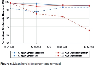
Indigenous versus alien plants plus Palmiet

In comparing the removal efficiencies of indigenous species and alien species currently implemented locally and internationally, the feasibility of replacing alien plants with local species was tested. Plants of similar physiology were selected for community comparison. The indigenous wetland species selected for this test included: Phragmites australis, Cyperus textilis, Typha capensis and Cynodon dactylon, which can be found in Renosterveld vegetation regions among others. The alien species were: Canna indica, Arundo donax and Pennisetum clandestinum. Prionium serratum, a South African indigenous plant species, is included with the alien assemblage due to its aggressive growth properties and absence in the agricultural area of interest in this study.

Figure 7 represents the mean percentage pollutants removed between the indigenous samples, the alien samples with Palmiet and the unvegetated soil control. It was inferred that there was no evidence that suggested one sample group to be more effective in removing pollutants than the other. It was however evident that both the Renosterveld and alien assemblages were more effective in the removal of pollutants than the unvegetated soil control. These comparative removal abilities of the two plant groups show the indigenous plant group to be as effective as internationally used species. This therefore supports the recommendation of rather implementing indigenous plants than their more invasive counterparts for remediation in sensitive contaminated sites.

 

 

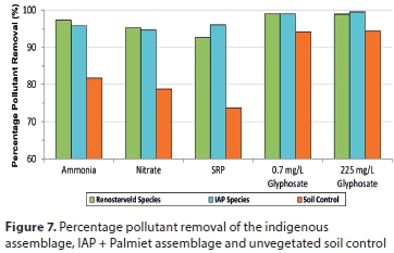
CONCLUSIONS

The designed system allowed for the evaluation of the phytoremediatory capabilities of selected plant species. This design and the use of the multiple plant silo allows for the comparison of indigenous species efficacy with that of alien plants commonly used for phytoremediation. The findings produced by the experimental system are comparable with literature from previous local and international studies, indicating the system accurately measures phytoremediatory capabilities of plant species. The system has been specifically designed to evaluate individual plant species of varying physiology and may thus be used to analyse species occupying different habitat types, i.e., wetland or dryland. Plant species can be successfully evaluated in terms of bioremediation capabilities, with the opportunity to incorporate different soil types (growth media) and pollutants. However, silo width plays a significant role, where pollutants are intercepted by a dense root system more effectively. The contaminants bind to the root structure and cell walls and hemicellulose within the cell wall and bind hydrophobic organic chemicals. The system is not limited to seasonal variability and conditions, granting the researcher the freedom to analyse pollutant remediation throughout the year. Further, proven effective plant species need to be investigated in a field setting, and with a cost analysis included.

 

ACKNOWLEDGEMENTS

This research was funded by The Rufford Foundation (UK), with project identity: [23296-1].

 

REFERENCES

BARCELO D (1997) Trace Determination of Pesticides and their Degradation Products in Water. Elsevier, Amsterdam.         [ Links ]

BELTRANO J, RUSCITTI M, ARANGO C and RONCO M (2013) Changes in the accumulation of shikimic acid in mycorrhized Capsicum annuum L. grown with application of glyphosate and phosphorus. Theoretical and Experimental Plant Physiol. 25 (2) 125-136. https://doi.org/10.1590/S2197-00252013000200005        [ Links ]

BRATIERES K, FLETCHER TD, DELETIC A and ZINGER Y (2008) Nutrient and sediment removal by stormwater biofilters: a large-scale design optimisation study. Water Res. 42 (14) 3930-3940. https://doi.org/10.1016/j.watres.2008.06.009        [ Links ]

BUNT AC (2012) Media and Mixes for Container-Grown Plants: A Manual on the Preparation and use of Growing Media for Pot Plants. Springer, London.         [ Links ]

CAMPBELL CS (1999) Constructed Wetlands in the Sustainable Landscape. John Wiley and Sons, New York.         [ Links ]

RSA (Republic of South Africa) (1996) Fertilizers, Farm Feeds, Agricultural Remedies and Stock Remedies Act. Act No. 36 of 1947. Government Printer, Pretoria.         [ Links ]

DAFF (Department of Agriculture, Forestry and Fisheries, South Africa) (2016) Production guideline for canola. DAFF, Pretoria.         [ Links ]

DONOSO G, CANCINO J and MAGRI A (1999) Effects of agricultural activities on water pollution with nitrates and pesticides in the Central Valley of Chile. Water Sci. Technol. 39 (3) 49-60. https://doi.org/10.2166/wst.1999.0134        [ Links ]

HASHEMI F, OLESEN JE, DALGAARD T and BØRGENSEN CD (2016) Review of scenario analyses to reduce agricultural nitrogen and phosphorus loading to the aquatic environment. Sci. Total Environ. 573 608-626. https://doi.org/10.1016/j.scitotenv.2016.08.141        [ Links ]

KENNEN K and KIRKWOOD N (2015) Phyto: Principles And Resources For Site Remediation And Landscape Design. Routledge, London. https://doi.org/10.4324/9781315746661        [ Links ]

LAM QD, SCHMALZ B and FOHRER N (2010) Modelling point and diffuse source pollution of nitrate in a rural lowland catchment using the SWAT model. Agric. Water Manage. 97 (2) 317-325. https://doi.org/10.1016/j.agwat.2009.10.004        [ Links ]

LEGUIZAMO MAO, GÓMEZ WDF and SARMIENTO MCG (2017) Native herbaceous plant species with potential use in phytoremediation of heavy metals, spotlight on wetlands: a review. Chemosphere 168 1230-1247. https://doi.org/10.1016/j.chemosphere.2016.10.075        [ Links ]

MILANDRI SG, WINTER KJ, CHIMPANGO SBM, ARMITAGE NP, MBUI DN, JACKSON GE and LIEBAU V (2012) The performance of plant species in removing nutrients from stormwater in biofiltration systems in Cape Town. Water SA 38 (5) 275-662.         [ Links ]

NORSE D (2005) Non-point pollution from crop production: Global, regional and national issues. Pedosphere 15 (4) 499-508.         [ Links ]

NORSE D, LI J, JIN L and ZHANG Z (2001) Environmental Costs of Rice Production in China: Lessons from Hunan and Hubei. Aileen International Press, Bethesda.         [ Links ]

OSRAM (2018) Biolux T8 Product data sheet. URL: http://www.osram.com/osram_com/products/lamps/fluorescentlamps/%0Afluorescent-lamps-t8/fluorescent-lamps-t8-special-versions/biolux-t8/index.jsp (Accessed 17 July 2017).         [ Links ]

PILON-SMITS E (2005) Phytoremediation. Annu. Rev. Plant Biol. 56 15-39. https://doi.org/10.1146/annurev.arplant.56.032604.144214        [ Links ]

READ J, FLETCHER TD, WEVILL T and DELETIC A (2010) Plant traits that enhance pollutant removal from stormwater in biofiltration systems. Int. J. Phytoremed. 12 (1) 34-53. https://doi.org/10.1080/15226510902767114        [ Links ]

READ J, WEVILL T, FLETCHER TD and DELETIC A (2008) Variation among plant species in pollutant removal from stormwater in biofiltration systems. Water Res. 42 (4-5) 893-902. https://doi.org/10.1016/j.watres.2007.08.036        [ Links ]

SCHACHTSCHNEIDER K, MUASYA M and SOMERSET V (2010) Are indigenous sedges useful for phytoremediation and wetland rehabilitation? Report no CSIR NE04-PO. CSIR, Pretoria.         [ Links ]

SCHOUMANS OF, CHARDON WJ, BECHMANN ME, GASCUEL-ODOUX C, HOFMAN G, KRONVANG B, RUBAEK GH, ULÉN B and DORIOZ JM (2014) Mitigation options to reduce phosphorus losses from the agricultural sector and improve surface water quality: a review. Sci. Total Environ. 468 1255-1266. https://doi.org/10.1016/j.scitotenv.2013.08.061        [ Links ]

SMITH LED and SICILIANO G (2015) A comprehensive review of constraints to improved management of fertilizers in China and mitigation of diffuse water pollution from agriculture. Agric. Ecosyst. Environ. 209 15-25. https://doi.org/10.1016/j.agee.2015.02.016        [ Links ]

TERRY N and BANUELOS GS (1999) Phytoremediation of Contaminated Soil and Water. Ringgold, Portland. https://doi.org/10.1201/9781439822654        [ Links ]

TESFAMARIAM T, BOTT S, CAKMAK I, RÖMHELD V and NEUMANN G (٢٠٠٩) Glyphosate in the rhizosphere - role of waiting times and different glyphosate binding forms in soils for phytotoxicity to non-target plants. Eur. J. Agron. 31 (3) 126-132. https://doi.org/10.1016/j.eja.2009.03.007        [ Links ]

WATERS (2018) Xevo TQ-XS Triple Quadrupole Mass Spectrometry. URL: http://www.waters.com/waters/en_ZA/Xevo-TQ-XS-Triple-Quadrupole-Mass-Spectrometry/nav.htm?cid=134889751&locale=en_ZA (Accessed 15 May 2018).         [ Links ]

 

 

Received 1 October 2018
Accepted in revised form 26 September 2019

 

 

* Corresponding author, email: janniedw@sun.ac.za

^rND^sBELTRANO^nJ^rND^sRUSCITTI^nM^rND^sARANGO^nC^rND^sRONCO^nM^rND^sBRATIERES^nK^rND^sFLETCHER^nTD^rND^sDELETIC^nA^rND^sZINGER^nY^rND^sDONOSO^nG^rND^sCANCINO^nJ^rND^sMAGRI^nA^rND^sHASHEMI^nF^rND^sOLESEN^nJE^rND^sDALGAARD^nT^rND^sBØRGENSEN^nCD^rND^sLAM^nQD^rND^sSCHMALZ^nB^rND^sFOHRER^nN^rND^sLEGUIZAMO^nMAO^rND^sGÓMEZ^nWDF^rND^sSARMIENTO^nMCG^rND^sMILANDRI^nSG^rND^sWINTER^nKJ^rND^sCHIMPANGO^nSBM^rND^sARMITAGE^nNP^rND^sMBUI^nDN^rND^sJACKSON^nGE^rND^sLIEBAU^nV^rND^sNORSE^nD^rND^sPILON-SMITS^nE^rND^sREAD^nJ^rND^sFLETCHER^nTD^rND^sWEVILL^nT^rND^sDELETIC^nA^rND^sREAD^nJ^rND^sWEVILL^nT^rND^sFLETCHER^nTD^rND^sDELETIC^nA^rND^sSCHOUMANS^nOF^rND^sCHARDON^nWJ^rND^sBECHMANN^nME^rND^sGASCUEL-ODOUX^nC^rND^sHOFMAN^nG^rND^sKRONVANG^nB^rND^sRUBAEK^nGH^rND^sULÉN^nB^rND^sDORIOZ^nJM^rND^sSMITH^nLED^rND^sSICILIANO^nG^rND^sTESFAMARIAM^nT^rND^sBOTT^nS^rND^sCAKMAK^nI^rND^sRÖMHELD^nV^rND^sNEUMANN^nG^rND^1A01^nSiqi^sWang^rND^1A01^nYinghua^sLi^rND^1A01^nHaibo^sLi^rND^1A01^nLei^sYang^rND^1A01^nSiqi^sWang^rND^1A01^nYinghua^sLi^rND^1A01^nHaibo^sLi^rND^1A01^nLei^sYang^rND^1A01^nSiqi^sWang^rND^1A01^nYinghua^sLi^rND^1A01^nHaibo^sLi^rND^1A01^nLei^sYang

RESEARCH PAPERS

 

Transport of pore-water oxygen with/without aeration in subsurface wastewater infiltration system

 

 

Siqi Wang; Yinghua Li^*; Haibo Li; Lei Yang

School of Resources and Civil Engineering, Northeastern University, Shenyang 110819, China

 

 

---

ABSTRACT

In this study, three subsurface wastewater infiltration systems (SWISs) at different aeration were set up to study the transport of pore-water oxygen and quantify the amount of trapped gas. Bromide and dissolved oxygen were introduced into SWISs as partitioning tracer and non-partitioning tracer, respectively. A model named CXTFIT based on the convection diffusion equation was used to describe the shape of breakthrough curves for bromide and dissolved air in column experiments. In CXTFIT code, the parameter β obtained from the bromide test ranging from 0.2940 to 0.7600 indicates that the physical non-equilibrium model was relatively suitable for dissolved air transport. Retardation factors obtained by CXTFIT code indicate 2-20% porosity filled with gas. Tracing the transport of air and determining the percentage of porosity filled with trapped gas has lain a foundation for further study on gas clogging in SWISs.

Keywords: gas-partitioning tracer, convection diffusion equation, subsurface wastewater infiltration system, dissolved air transport, gas clogging

---

 

 

INTRODUCTION

Subsurface wastewater infiltration systems (SWISs) are effective wastewater treatment methods due to the integrated mechanism of chemical, physical and biological reactions, as wastewater passes through the unsaturated soil in SWISs (Jiang, 2017). SWISs are widely used due to their low operation cost, easy maintenance, and low energy consumption (Li, 2017b).

Unfortunately, SWISs have the disadvantage of poor performance if clogging occurs. Clogging can be divided into four types: physical clogging (caused by suspended solids) (Yang, 2018; Alem, 2015); bioclogging (caused by accumulated biofilms) (Newcomer, 2016; Hua, 2014); chemical clogging (caused by chemical materials such as carbonate and iron oxide ) (Larroque, 2011; Weidner, 2012); and gas clogging (caused by gas bubbles) (Heilweil, 2013). Currently, researchers are devoted to the study of physical clogging, bioclogging and chemical clogging, but little is known about gas clogging. Gas bubbles can block pore throats, increasing the resistance to flow and reducing permeability (Martin, 2013). To study gas clogging, the sources and characteristics of gas in SWISs need to be understood.

The presence of gas bubbles in SWISs has been attributed to the biogenic gas and entrapped air. Previous studies have investigated biogenic gas. Nitrogen and nitrous oxide are produced by nitrification and denitrification. The impacts of influent loadings, drying-wetting cycles and carbon-nitrogen ratio on nitrous oxide emission and spatial distribution of nitrous oxide have been studied by Ying-Hua Li (Li, 2017a; Li, 2018). N₂O conversion rate decreased with an increase in hydraulic loading (HL) but increased with increasing pollutant loading (PL) (Li, 2017a). A moderate carbon-nitrogen ratio leads to an increase in N₂O emission rate and the 0-75 cm depth layer was the main contributor to N₂O emissions (Li, 2018).

However, there is limited knowledge on the pathways of entrapped air transportation. Dissolved gases carried with the influent were a major source of entrapped air bubbles. Compared to a saturated system, dissolved gases are more inclined to separate from the influent and penetrate into small pores in an unsaturated system like a SWIS. Entrapped air bubbles are no longer connected to the atmosphere, occurring in the form of small, immobilized, disconnected bubbles (Heilweil, 2013). By reducing the effective (quasi-saturated) hydraulic conductivity, entrapped air bubbles impact water flow and solute and contaminant transport (Marinas, 2013). In order to research entrapped air, a gas-partitioning tracer test was introduced to distinguish between two fluid phases. The gas-partitioning tracer test was initially used to determine residual oil saturation by the petroleum industry (Tang, 1991a; Tang, 1991b). This has been applied more recently for the movement of air in the non-saturated zone and to measure air-filled porosity. Both a partitioning tracer and a non-partitioning tracer are injected simultaneously with influent and measured in effluent. A partitioning tracer, the low-solubility dissolved gas, will partition to the gas phase partially while a non-partitioning tracer stays in the liquid phase, which results in a partitioning tracer travelling at a lower velocity than a non-partitioning tracer. Common partitioning tracers are oxygen (Fry, 1996) and noble gas (e.g. helium, neon and argon) (Burnard, 2013; Reid, 2013). Common non-partitioning tracers are chloride and bromide. A series of transport experiments showed that the presence of small amounts of entrapped gas in the pore space could result in retardation factors for dissolved oxygen (Fry, 1995). The retardation factor is interpreted as the ratio of groundwater velocity to dissolved gas velocity and Fry reported retardation factors for dissolved oxygen varying from 1.0 to 8.0 (Fry, 1995). Higher retardation factors indicate more entrapped air. Heilweil used retardation factors obtained from a gas partitioning tracer to quantify entrapped gas in an infiltration experiment and indicated that 7% to more than 26% of the porosity was filled with gas (Heilweil, 2004). Vulave (2002) used dissolved Kr and SF₆ gases to determine hydrogeological parameters. Through there were lower aqueous diffusion coefficients for SF₆ than that for Kr, both Kr and SF₆ can be used with confidence to delineate and validate aquifer characteristics. It is noted that there is a special gas-partitioning tracer test referred as the 'Push-Pull' test (PPT). In the 'Push-Pull' test, a partitioning tracer and a non-partitioning tracer are injected ('pushed') into a porous media and then extracted ('pulled') in situ. Reid exploited the 'Push-Pull' test to research dissolved gas dynamics in wetland soils (Reid, 2015).

In this study, laboratory experiments were conducted, combined with numerical simulations, with the aim of achieving better understanding of the transport of dissolved air under various aeration conditions and quantifying the amount of trapped gas in SWISs. Tracing the transport of air and determining the percentage of porosity filled with trapped gas has lain the foundation for further studies on gas clogging in SWISs.

 

MATERIALS AND METHODS

System description

The soil column made of plexiglass was constructed (height 180 cm and internal diameter 29 cm) and operated indoors. The 145 cm high substrate was built on top of 5 cm of gravel (0.6-0.9 cm, diameter). The substrate was evenly mixed with sand, slag and farmland soil at a ratio of 1:2.5:6.5. The porosity of the substrate was 55.0%. The gravel at the bottom was used to support the infiltration system, evenly distribute the treated water and prevent outlet blockage. Influent from the water tank to the column was pumped with a peristaltic pump and distributed via a 2-cm-diameter perforated water distribution pipe placed at 65 cm depth under the soil. The water was purified by the substrate and finally collected at the outlet. Rhizon soil solution samplers were placed at 40, 70, 100 and 130 cm depths (Fig. 1).

 

 

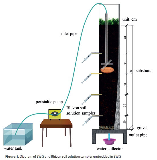
Wastewater

Artificial domestic wastewater was prepared with tap water including glucose, ammonium chloride, potassium nitrate, sodium nitrite and monopotassium phosphate. The parameters of the wastewater were as follows: COD 330.21 ± 7 mg/L, NO₃⁻-N 3.12 ± 0.1 mg/L, NO₂⁻-N 0.40 ± 0.004 mg/L, NH₄⁺-N 49.08 ± 0.6 mg/L, TP 4.0 ± 0.3 mg/L. The domestic wastewater was treated in different ways to form the following 4 kinds of water:

•Degassed water (DW): The domestic wastewater was filtered through a degasification membrane. DO concentration was 2.0 mg/L.

•Non-aerated water (NW): The domestic wastewater without any treatment. DO concentration was 6.0 mg/L, the same as that of tap water.

•Micro-aerated water (MW): The domestic wastewater was continuously aerated by a 45 L/min aeration pump. DO concentration was 9.1 mg/L. Gas bubble content was 3.6%. Gas content was measured following the method of Du (2016).

•Aerated water (AW): The domestic wastewater was aerated continuously by a 70 L/min aeration pump. DO concentration was 9.2 mg/L. Gas bubble content was 6.3%.

Gas-partitioning tracer test operation

Bromide tracer test

Phenol was added to the four types of water (DW, NW, MW and AW) as a biocide to prevent biological consumption of oxygen. Phenol concentration was 1%. When the operation of the system was steady, DW was dosed in the SWIS for the first time for several days to maintain the same initial conditions. Table 1 shows measured DO concentrations after DW was injected for several days. Potassium bromide (KBr) was added to the influent and Br⁻ concentration was 10 g/L. The influent with KBr was injected for 4 h via a peristaltic pump. Then DW was introduced to the SWIS for the second time for about 4 days to discharge all KBr. The hydraulic loading was 0.14 m/d. Water samples were collected at 40, 70, 100, 130 and 150 cm depths. KBr was measured to get breakthrough curves at different depths. KBr, a non-partitioning tracer without retardation, was used to select an adaptive model and parameters for the transport of DO.

 

 

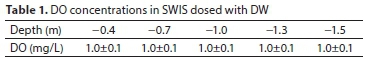
Oxygen tracer test

Instead of the influent with KBr, NW, MW and AW were injected for 4 h after dosing DW for the first time. All other experimental procedures were the same as for bromide tracer test. With the model and parameters acquired from bromide tracer test, DO concentrations were measured to get breakthrough curves at different depths and various aerations. Aeration with air was used to increase air content, i.e., increase oxygen content; the transport of DO represents the transport of air.

Numerical simulations

CXTFIT code was developed by the U.S. Salinity Laboratory. Based on the convection-dispersion equation (CDE), CXTFIT code is a model developed to estimate parameters in equilibrium and non-equilibrium transport from laboratory or field tracer experiments (Toride, 1995). CXTFIT allows for analyses of concentration distributions versus time as well as depth, and permits the use of the equilibrium and non-equilibrium transport formulations (Van Genuchten, 2012).

In CXTFIT code, the dimensionless form of equilibrium transport according to the convection-dispersion equation (CDE) is written as:

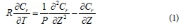
where R is retardation factor, C_r is the dimensionless solute concentration, T is the dimensionless time, P is the Peclet number, Z is the dimensionless distance. The following equations define the dimensionless parameters:

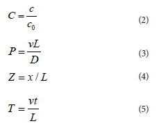
where c is the measured concentration (g/L or mg/L), c₀ is the initial concentration (g/L or mg/L), x is distance (m), L is the characteristic length (m) representing the column length, D is the dispersion coefficient (m²/d), t is time (d), v is the average pore-water velocity (m/d).

In CXTFIT code, the non-equilibrium transport includes chemical and physical non-equilibrium processes. The chemical non-equilibrium can be described by a two-site non-equilibrium model. The two-site non-equilibrium model divides adsorption sites into instantaneous equilibrium adsorption sites and non-equilibrium adsorption sites governed by first-order kinetics. The two-site non-equilibrium model reduced to the dimensionless form can be written as:

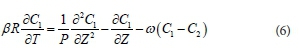
where β is a partitioning coefficient, ω is a dimensionless mass transfer coefficient, and the subscripts 1 and 2 represent the (mobile) liquid phase and the (immobile) trapped gas phase, respectively.

The physical non-equilibrium can be described by a two-region non-equilibrium model. The two-region non-equilibrium model supposes that the liquid phase can be partitioned into mobile and immobile regions. Mass transfer between the two regions is simulated as a first-order process. The two-region non-equilibrium model reduced to the dimensionless form can be written as:

In this study, the equilibrium and physical non-equilibrium model in CXTFIT code was used to simulate breakthrough and elution curves of KBr and DO in SWISs. CXTFIT code uses a non-linear least-square optimization approach based on the Levenberg-Marquardt method to estimate unknown parameters (Toride, 1995). R is fixed as 1 due to no retardation for non-partitioning tracers such as bromide. For equilibrium transport, CXTFIT code is used to fit D and v. For non-equilibrium transport, v is the set value, CXTFIT code is used to fit D. Partitioning tracers have same D and v with non-partitioning tracers. For partitioning tracers such as oxygen, D and v are fixed to be the same as for non-partitioning tracers. CXTFIT code is used to fit R in equilibrium transport and R, β as well as ω in non-equilibrium transport.

Sampling and analytical methods modification

Water sampling was done at 40, 70, 100 and 130 cm depths via Rhizon soil solution samplers and effluent was collected at 150 cm depth.

Bromide was measured via the phenol red spectrophotometric method (Tomiyasu, 1996). The phenol red spectrophotometric method is suitable for low concentrations nd water samples should be diluted. DO concentrations were measured using a dissolved oxygen meter.

Method to quantify trapped gas

Fry put forward the following equation to describe the retardation factor (Fry, 1995):

where H′ is dimensionless Henry's law constant, V_g is volume of trapped gas per volume of pore space and V_w is volume of water per volume of pore space.

With R from CXTFIT code and dimensionless Henry's law constants for oxygen from Fry's research (Fry, 1995), the percentage of gas-filled porosity can be obtained by the following equation:

where θ_g is the per cent gas-filled porosity.

 

RESULTS AND DISCUSSION

Transport of bromide

Figure 2 shows bromide transport at different depths in SWISs. The peak measured bromide concentration reached 7.83 g/L (C/C₀ = 0.783) at 4 h (T = 0.028) and 0.7 m from the surface, due to the nearby water distribution pipe placed at 0.65 m depth under the soil. After bromide was injected for the first 4 h, the measured bromide concentration decreased rapidly to zero at 0.7 m from the surface. Under capillarity action, water travelled upward and the peak measured bromide concentration reached 1.07 g/L (C/C₀= 0.107) at 6 h (T = 0.042) and 0.4 m from the surface. Subsequently, water moved down along the column. The time to reach peak measured bromide concentration was 12 h (T = 0.085), 32 h (T = 0.226) and 58 h (T = 0.410) at 1.0, 1.3, 1.5 m from the surface, respectively. Except for 0.4 m from the surface, the peak measured bromide concentrations decreased with increasing depth.

 

 

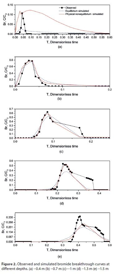
The bromide tracer test not only showed the transport of non-partitioning tracer, but was also used to choose a suitable model and parameters for the transport of DO. The constraint for the chemical non-equilibrium model is that 1/R ≤ β ≤ 0.9999. Because R is fixed as 1 in the simulation of non-partitioning tracers, the chemical non-equilibrium model is unfit for the transport of bromide. As shown in Fig.2, the equilibrium and physical non-equilibrium model were exploited to simulate bromide transport. Table 2 presents the fitted model parameters in the equilibrium and physical non-equilibrium model. Both the equilibrium and physical non-equilibrium model didn't fit bromide transport at 0.4 m. Compared with the equilibrium model, the physical non-equilibrium model was more suitable for bromide transport due to higher r². In the physical non-equilibrium model, the simulation was strong and significant with r² > 0.8 at 0.7, 1.0, 1.3, 1.5 m under the soil while it was very weak at 0.4 m under the soil (CXTFIT code didn't obtain a correlation coefficient). The highest dispersivity (0.01488 m) at 0.7 m under the soil was probably due to water distributed nearby, which meant much more complicated water flow conditions than other positions. The dispersivity increased from 2.712 × 10⁻³ to 7.280 × 10⁻³ m with depths from 1.0 to 1.5 m under the soil. The partitioning coefficient, β, determines the distribution of soil water between mobile and immobile regions. Through water in immobile regions doesn't move, mass exchange between mobile and immobile regions is carried out by molecular diffusion. β ranged from 0.2940 to 0.7600 (except for 0.4 m under the soil), which meant that mobile regions accounted for 0.2940 to 0.7600 of the soil water and the other was immobile regions, which also had a wide range of values. A wide range of immobile regions indicates that immobile regions played an important role in bromide transport and the physical non-equilibrium couldn't be neglected. The asymmetric breakthrough of bromide also proved the importance of immobile regions. Therefore the physical non-equilibrium model was shown to be suitable for bromide transport. With v and D obtained by bromide transport in Table 2, the physical non-equilibrium was used to simulate oxygen transport.

 

 

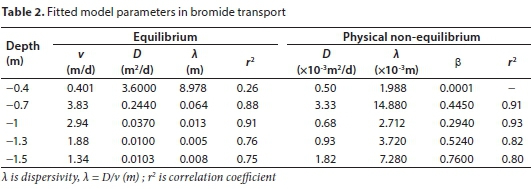
Transport of dissolved air in NW

Figure 3 shows the transport of oxygen in NW. DO concen-trations greater than 2.0 mg/L commonly refer to aerobic environments, while less than 0.2 mg/L represents anaerobic environments (Pan, 2016). DO concentration was 5.0 mg/L at 0.7 m under the soil, attributed to dissolved air carried by influent. DO climbed up first and then flowed down along the water's pathway. Without biological consumption of oxygen, DO could reach as deep as 1.0 m under the soil. All DO concentrations stabilized to be about 0.9 mg/L after 30 h, indicating that the system with NW was under an anoxic environment. DO concentrations remained at about 0.9 mg/L at 1.3 and 1.5 m under the soil for the whole run, revealing that DO couldn't run through the whole column due to dissolved air partitioning to gas phase. The time of the peak measured DO concentrations was at 7 h, 6 h, and 14 h at 0.4, 0.7, and 1.0 m under the soil. Comparing the breakthrough curves of DO at 0.4, 0.7 and 1.0 m under the soil with bromide, the time of peak measured DO concentrations was later than peak measured bromide at 0.4, 0.7 and 1.0 m under the soil, which is referred to as retardation.

 

 

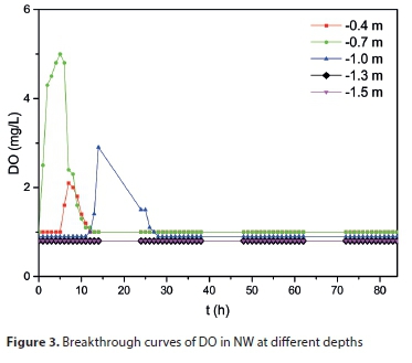
The simulated DO breakthrough curves and model parameters are presented in Fig. 4 and Table 3, respectively. Retardation factors ranged from 1.5-7.8 indicating 1.6-18.3% pore space was filled with gas. 1.6-18.3% of the pore space was filled with gas, mainly occurring at 0.65-1.0 m under the soil. DO couldn't run through the whole column, so R at −1.3 m and −1.5 m couldn't be obtained, thus pore space filled with gas at −1.3 m and −1.5 m couldn't be determined. A possible explanation for the low percentage of gas-filled porosity at 0.7 m under the soil is that the influent was distributed nearby and drove away the gas. With water moving down along the column, the dissolved air in water would gradually partition to the gas phase, resulting in higher gas-filled porosity at a deeper position.

 

 

 

 

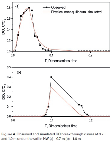
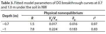
In oxygen tracer tests, C and C₀ was obtained by measured values minus the background values in Table 1.

Transport of dissolved air in MW

Breakthrough curves of DO in MW at different depths are shown in Fig. 5. The peak measured DO concentrations in MW were higher than NW at all depths. The low DO concentrations were measured at 48-49 h and 1.3 m under the soil. That deeper DO reach position can be explained by higher initial DO concentrations due to aeration.

 

 

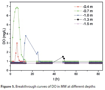
The simulated DO breakthrough curves and model parameters are presented in Fig. 6 and Table 4, respectively. Although DO concentrations were measured at 1.3 m under the soil, the measured values were too few to obtain a simulated curve. Retardation factors ranging from 1.4-8.1 indicate 1.3-23.4% pore space filled with gas.

 

 

 

 

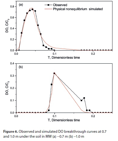
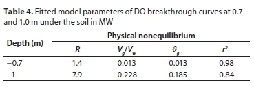
Transport of dissolved air in AW

Breakthrough curves of DO in AW at different depths are shown in Fig. 7. Compared to the breakthrough curves of DO in NW, MW and AW, breakthrough curves showed a similar shape and tendency. Both peak measured DO concentrations in MW and AW were much higher than in NW, mirroring that aeration improved the aerobic and anaerobic conditions in the substrate. The peak measured DO concentration at 0.7 m under the soil in AW was almost the same as in MW. But the peak measured DO concentration at 1.0 m under the soil in AW was a little higher than in MW, which is probably due to the higher gas content in AW than in MW. DO concentrations in MW and AW were both measured at 1.3 m under the soil, reflecting that higher DO concentrations could cause deeper breakthrough positions.

 

 

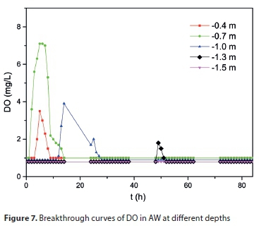
The simulated DO breakthrough curves and model parameters are presented in Fig. 8 and Table 5, respectively. Simulations of NW, MW and AW produce better model fitting at 0.7 m under the soil and relatively worse fitting at 1.0 m under the soil. This is probably because water climbing to 0.4 m under the soil moved down to 1.0 m under the soil and affected the simulation effect. At 0.7 m under the soil, the measured DO concentrations were relatively high and water climbing to 0.4 m under the soil had little effect. Retardation factors indicate 1.9-17.1% of porosity filled with gas. Retardation factors remained similar at various aerations. Two possible causes can explain this phenomenon: (i) When gases in dissolved air (e.g. nitrogen, oxygen, carbon dioxide, noble gas) partition to the gas phase, gases in the gas phase (e.g. nitrogen, nitrous oxide, methane, nitrogen dioxide) partition to the liquid phase simultaneously. Gas exchange between the gas phase and the liquid phase reach equilibrium, keeping almost unchanged the percentage of porosity filled with gas. (ii) Gases in dissolved air partitioning to the gas phase move with the mobile water, resulting in a stable percentage of porosity filled with gas.

 

 

 

 

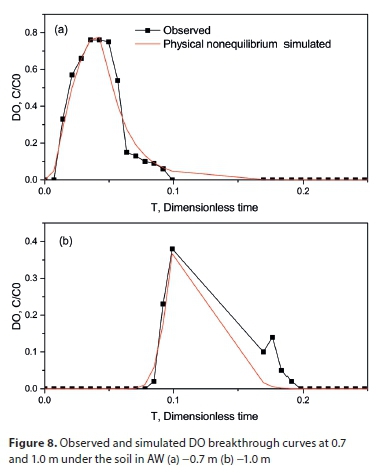
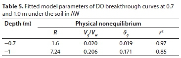
CONCLUSIONS

•CXTFIT code was first used to study dissolved air transport in SWISs. The parameter β, ranging from 0.2940 to 0.7600, indicates that immobile regions crucially affect solute transport. So the physical non-equilibrium model was suitable for DO transport.

•DO breakthrough curves shows the process of oxygen transport. Only a small amount of DO climbed up with the water. Higher DO concentrations resulted in reaching deeper positions. Saturated DO could reach 1.3 m under the soil and couldn't travel through the whole soil column (1.5 m). Oxygen was added by aeration, which means dissolved oxygen transport can represent dissolved air transport.

•Retardation factors of DO indicated 2-20% of pore space was filled with gas. Different aeration had similar retardation factors at each depth, reflecting the percentage of porosity filled with gas remained almost the same at each depth in SWISs and higher DO or gas content in wastewater had little effect on the percentage of porosity filled with gas.

Dissolved air transport is the basis of gas clogging. Based on this preliminary study, gas clogging can be relieved by reducing bubble accumulation. Therefore, a substrate with good permeability can prevent gas clogging. The mechanism of gas clogging requires further investigation.

 

ACKNOWLEDGEMENTS

This work was financially supported by the National Natural Science Foundation of China [grant numbers 41571455, 51578115] and Basic Science Research Fund for Northeastern University [grant number 160104004].

 

REFERENCES

ALEM A, AHFIR ND, ELKAWAFI A and WANG H (2015) Hydraulic operating conditions and particle concentration effects on physical clogging of a porous medium. Transp. Por. Media 106 (2) 303-321. https://doi.org/10.1007/s11242-014-0402-8.         [ Links ]

BURNARD P (2013) The Noble Gases as Geochemical Tracers. Springer, New York. 391 pp. https://doi.org/10.1007/978-3-642-28836-4        [ Links ]

DU L (2016) Experimental study on gas phase clogging in aquifer recovery. Doctoral dissertation, Ji′nan University. (in Chinese) DOI: 10.14042/j.cnki.32.1309.2017.05.013.         [ Links ]

FRY VA, ISTOK JD, SEMPRINI L, O'REILLY KT and BUSCHECK TE (1995) Retardation of dissolved oxygen due to a trapped gas phase in porous media. Groundwater 33 (3) 391-398. https://doi.org/10.1111/j.1745-6584.1995.tb00295.x        [ Links ]

FRY VA, ISTOK JD and O'REILLY KT (1996) Effect of trapped gas on dissolved oxygen transport-Implications for in situ bioremediation. Groundwater 34 (2) 200-210. https://doi.org/10.1111/j.1745-6584.1996.tb01880.x        [ Links ]

HEILWEIL VM and MARSTON T (2013) Evaluation of potential gas clogging associated with managed aquifer recharge from a spreading basin, Southwestern Utah, USA. In: Clogging Issues Associated With Managed Aquifer Recharge Methods. IAH Commission on Managing Aquifer Recharge, Australia. ISBN: 978-0-646-90852-6.         [ Links ]

HEILWEIL VM, KIP SOLOMON D, PERKINS KS and ELLETT KM (2004) Gas‐partitioning tracer test to quantify trapped gas during recharge. Groundwater 42 (4) 589-600. https://doi.org/10.1111/j.1745-6584.2004.tb02627.x        [ Links ]

HUA G, ZENG Y, ZHAO Z, CHENG K and CHEN G (2014) Applying a resting operation to alleviate bioclogging in vertical flow constructed wetlands: an experimental lab evaluation. J. Environ. Manage. 136 47-53. https://doi.org/10.1016/j.jenvman.2014.01.030        [ Links ]

JIANG Y, SUN Y, PAN J and ZHANG Y (2017) Use of dewatered sludge as microbial inoculum of a subsurface wastewater infiltration system: effect on start-up and pollutant removal. Water SA 43 (4) 595-601. https://doi.org/10.4314/wsa.v43i4.07        [ Links ]

LARROQUE F and FRANCESCHI M (2011) Impact of chemical clogging on de-watering well productivity: numerical assessment. Environ. Earth Sci. 64 (1) 119-131. https://doi.org/10.1007/s12665-010-0823-9        [ Links ]

LI YH, LI HB, XU XY, XIAO SY, WANG SQ and XU SC (2017a) Field study on N₂O emission from subsurface wastewater infiltration system under variable loading rates and drying-wetting cycles. Water Sci. Technol. 76 (8) 2158-2166. https://doi.org/10.2166/wst.2017.388        [ Links ]

LI YH, LI HB, XU XY, XIAO SY, WANG SQ and XU SC (2017b) Fate of nitrogen in subsurface infiltration system for treating secondary effluent. Water Sci. Eng. 10 (3) 217-224. https://doi.org/10.1016/j.wse.2017.10.002        [ Links ]

LI YH, LI HB, XU XY, WANG SQ and PAN J (2018) Does carbon-nitrogen ratio affect nitrous oxide emission and spatial distribution in subsurface wastewater infiltration system? Bioresour. Technol. 250 846-852. https://doi.org/10.1016/j.biortech.2017.12.024        [ Links ]

MARINAS M, ROY JW and SMITH JE (2013) Changes in entrapped gas content and hydraulic conductivity with pressure. Groundwater 51 (1) 41-50. https://doi.org/10.1111/j.1745-6584.2012.00915.x        [ Links ]

MARTIN R (2013) Clogging Issues Associated With Managed Aquifer Recharge Methods. IAH Commission on Managing Aquifer Recharge, Australia.8 pp. ISBN: 978-0-646-90852-6.         [ Links ]

NEWCOMER ME, HUBBARD SS, FLECKENSTEIN JH, MAIER U, SCHMIDT C, THULLNER M, ULRICH G, FLIPO N and RUBIN Y (2016) Simulating bioclogging effects on dynamic riverbed permeability and infiltration. Water Resour. Res. 52 (4) 2883-2900. https://doi.org/10.1002/2015WR018351        [ Links ]

PAN J, YUAN F, ZHANG Y, HUANG L, CHENG F, ZHENG F and LIU R (2016) Nitrogen removal in subsurface wastewater infiltration systems with and without intermittent aeration. Ecol. Eng. 94 471-477. https://doi.org/10.1016/j.ecoleng.2016.06.025        [ Links ]

REID MC and JAFFÉ PR (2013) A push-pull test to measure root uptake of volatile chemicals from wetland soils. Environ. Sci. Technol. 47 (7) 3190-3198. https://doi.org/10.1021/es304748r        [ Links ]

REID MC, PAL DS and JAFFÉ PR (2015) Dissolved gas dynamics in wetland soils: Root‐mediated gas transfer kinetics determined via push‐pull tracer tests. Water Resour. Res. 51 (9) 7343-7357. https://doi.org/10.1002/2014WR016803        [ Links ]

TOMIYASU T, TAGA Y, SAKAMOTO H and YONEHARA N (1996) Spectrophotometric determination of trace bromide by its catalytic effect on the tetrabase-chloramine T reaction. Anal. Chim. Acta 319 (1-2) 199-204. https://doi.org/10.1016/0003-2670(95)00490-4        [ Links ]

TANG JS and HARKER BJ (1991a) Interwell tracer test to determine residual oil saturation in a gas-saturated reservoir, Part 1. Theory and design. J. Can. Petrol. Technol. 30 (3) 76-85. https://doi.org/10.2118/91-03-08        [ Links ]

TANG JS and HARKER BJ (1991b) Interwell tracer test to determine residual oil saturation in a gas-saturated reservoir, Part 2: Field applications. J. Can. Petrol. Technol. 30 (4) 34-42. https://doi.org/10.1016/0148-9062(92)93816-3        [ Links ]

TORIDE N, LEIJ FJ and VAN GENUCHTEN MT (1995) The CXTFIT code for estimating transport parameters from laboratory or field tracer experiments. Research Report No. 137. US Salinity Laboratory, US Dept of Agriculture.         [ Links ]

VAN GENUCHTEN MT, ŠIMUNEK J, LEIJ FJ, TORIDE N and ŠEJNA M (2012) STANMOD: Model use, calibration, and validation. Trans. ASABE 55 (4) 1355-1366. https://doi.org/10.13031/2013.42247        [ Links ]

VULAVA VM, PERRY EB, ROMANEK CS and SEAMAN JC (2002). Dissolved gases as partitioning tracers for determination of hydrogeological parameters. Environ. Sci. Technol. 36 (2) 254-262. https://doi.org/10.1021/es0107024        [ Links ]

WEIDNER C, HENKEL S, LORKE S, RÜDE TR, SCHÜTTRUMPF H and KLAUDER W (2012) Experimental modelling of chemical clogging processes in dewatering wells. Mine Water Environ. 31 (4) 242-251. https://doi.org/10.1007/s10230-012-0188-2        [ Links ]

YANG M, LU M, BIAN H, SHENG L and HE C (2018) Effects of physical clogging on the performance of a lab-scale vertical subsurface flow constructed wetland system and simulation research. Ecol. Indic. 92 11-17. https://doi.org/10.1016/j.ecolind.2017.05.058        [ Links ]

 

 

Received 20 November 2018
Accepted in revised form 25 September 2019

 

 

* Corresponding author, email: liyinghua@mail.neu.edu.cn

^rND^sALEM^nA^rND^sAHFIR^nND^rND^sELKAWAFI^nA^rND^sWANG^nH^rND^sFRY^nVA^rND^sISTOK^nJD^rND^sSEMPRINI^nL^rND^sO'REILLY^nKT^rND^sBUSCHECK^nTE^rND^sFRY^nVA^rND^sISTOK^nJD^rND^sO'REILLY^nKT^rND^sHEILWEIL^nVM^rND^sMARSTON^nT^rND^sHEILWEIL^nVM^rND^sKIP SOLOMON^nD^rND^sPERKINS^nKS^rND^sELLETT^nKM^rND^sHUA^nG^rND^sZENG^nY^rND^sZHAO^nZ^rND^sCHENG^nK^rND^sCHEN^nG^rND^sJIANG^nY^rND^sSUN^nY^rND^sPAN^nJ^rND^sZHANG^nY^rND^sLARROQUE^nF^rND^sFRANCESCHI^nM^rND^sLI^nYH^rND^sLI^nHB^rND^sXU^nXY^rND^sXIAO^nSY^rND^sWANG^nSQ^rND^sXU^nSC^rND^sLI^nYH^rND^sLI^nHB^rND^sXU^nXY^rND^sXIAO^nSY^rND^sWANG^nSQ^rND^sXU^nSC^rND^sLI^nYH^rND^sLI^nHB^rND^sXU^nXY^rND^sWANG^nSQ^rND^sPAN^nJ^rND^sMARINAS^nM^rND^sROY^nJW^rND^sSMITH^nJE^rND^sNEWCOMER^nME^rND^sHUBBARD^nSS^rND^sFLECKENSTEIN^nJH^rND^sMAIER^nU^rND^sSCHMIDT^nC^rND^sTHULLNER^nM^rND^sULRICH^nG^rND^sFLIPO^nN^rND^sRUBIN^nY^rND^sPAN^nJ^rND^sYUAN^nF^rND^sZHANG^nY^rND^sHUANG^nL^rND^sCHENG^nF^rND^sZHENG^nF^rND^sLIU^nR^rND^sREID^nMC^rND^sJAFFÉ^nPR^rND^sREID^nMC^rND^sPAL^nDS^rND^sJAFFÉ^nPR^rND^sTOMIYASU^nT^rND^sTAGA^nY^rND^sSAKAMOTO^nH^rND^sYONEHARA^nN^rND^sTANG^nJS^rND^sHARKER^nBJ^rND^sTANG^nJS^rND^sHARKER^nBJ^rND^sVAN GENUCHTEN^nMT^rND^sŠIMUNEK^nJ^rND^sLEIJ^nFJ^rND^sTORIDE^nN^rND^sŠEJNA^nM^rND^sVULAVA^nVM^rND^sPERRY^nEB^rND^sROMANEK^nCS^rND^sSEAMAN^nJC^rND^sWEIDNER^nC^rND^sHENKEL^nS^rND^sLORKE^nS^rND^sRÜDE^nTR^rND^sSCHÜTTRUMPF^nH^rND^sKLAUDER^nW^rND^sYANG^nM^rND^sLU^nM^rND^sBIAN^nH^rND^sSHENG^nL^rND^sHE^nC^rND^1A01 A02^nLe Anh^sPham^rND^1A01^nJulien^sLaurent^rND^1A01^nPaul^sBois^rND^1A01^nAdrien^sWanko^rND^1A01 A02^nLe Anh^sPham^rND^1A01^nJulien^sLaurent^rND^1A01^nPaul^sBois^rND^1A01^nAdrien^sWanko^rND^1A01 A02^nLe Anh^sPham^rND^1A01^nJulien^sLaurent^rND^1A01^nPaul^sBois^rND^1A01^nAdrien^sWanko

RESEARCH PAPERS

 

Finding optimal algal/bacterial inoculation ratio to improve algal biomass growth with wastewater as nutrient source

 

 

Le Anh Pham^{I, II}; Julien Laurent^{I, *}; Paul Bois^I; Adrien Wanko^I

^IICube, UMR 7357, ENGEES, CNRS, Université de Strasbourg, 2 rue Boussingault, 67000 Strasbourg, France
^IIDepartment of Water-Environment-Oceanography, University of Science and Technology of Hanoi, Vietnam Academy of Science and Technology, 18 Hoang Quoc Viet, Hanoi, Vietnam

 

 

---

ABSTRACT

Algal growth, nutrient removal and settling efficiency were quantified while inoculating sequencing batch reactors with a mixture of microalgae and bacteria (activated sludge). Three algae/bacteria inoculation ratios (5:1, 1:1 and 1:5) as well as pure algal biomass (control) were assessed. Algal biomass production increased with the addition of activated sludge. However, the addition of too much activated sludge can cause disturbance to the Al-Bac biomass growth and algal bacterial processes. All reactors including the control with only algae showed similar settling and nutrient removal efficiencies. Good settling was observed in all reactors with only 5% of total biomass found in supernatant after 1 h of settling. Removal efficiencies of COD, TN and PO₄-P in all reactors were 79-82%, 61-65% and 15-37%, respectively, with the lowest phosphorus removal efficiency belonging to 1:5 algae/activated sludge ratio. These results may be due to both long hydraulic (7 days) and solids retention times (up to 30 days). Finally, Al-Bac biomass with 1:1 inoculation ratio showed the best enhancement in terms of biomass growth and algal activities.

Keywords: microalgae, activated sludge, nutrients, wastewater, sequencing batch reactor

---

 

 

INTRODUCTION

The role of microalgae in wastewater treatment for photosynthetic aeration has been recognized for a long time (Oswald and Gotaas, 1957). Microalgae provide O₂ to heterotrophic aerobic bacteria that oxidize organic pollution for their growth and energy requirements, using in turn the CO₂ released from bacterial respiration for algal photosynthesis. This process is naturally driven, requiring only natural light for algal photosynthesis and hence significantly reducing operation costs as well as the carbon footprint of the wastewater treatment system, especially in comparison with conventional activated sludge technology (Van Den Hende et al., 2014). Moreover, during their growth, algal cells might accumulate high amount of lipids and carbohydrates. Hence algal biomass can be used as raw material for anaerobic digestion to produce biomethane or chemical extraction for biofuel production (Sirajunnisa and Surendhiran, 2016; Voloshin et al., 2016). Over the past few years, the use of microalgae for biomass production and wastewater treatment has received considerable attention and has been extensively studied (Park et al., 2011; Sutherland et al., 2015).

However, small cell size and low concentration in culture solution hampers efficient harvesting of algal biomass from water. An efficient harvesting process may account for up to 20 to 30% of total production cost (Mata et al., 2010; Pragya et al., 2013). Algae harvesting remains, therefore, one of the biggest challenges when operating these type of systems (Uduman et al., 2010; Christenson and Sims, 2011; Craggs et al., 2015). One possible solution might be to enhance algal biomass settleability by bio-flocculation (Salim et al., 2010; Vandamme et al., 2013). Indeed, inoculating activated sludge with algae in wastewater has been shown to improve biomass settling while maintaining good treatment efficiency (Gutzeit et al., 2005; Van Den Hende et al., 2011). Studies on algal-bacterial biomass indicated high gravitational settling efficiencies by flocculation between algae and bacteria (Gutzeit et al., 2005; Medina and Neis, 2007; Van Den Hende et al., 2014). Van Den Hende et al. (2014) recovered nearly 100% of algal-bacterial biomass from a pilot scale study via two simple harvesting steps, including gravity settling and dewatering by filter press, requiring no chemical addition or electricity. Most of these promising results, however, were achieved on pilot or semi-industrial scale. Although the potential of this technology is recognized, research on improving algal production while maintaining treatment efficiency is still needed before the system can be applied on an industrial scale (Park et al., 2011).

When co-culturing algae and bacteria, one important factor impacting algal growth is the inoculation ratio. Su et al. (2012b) reported that algae/activated sludge ratio of 5:1 was optimal to achieve good wastewater treatment and biomass settling. Roudsari et al. (2014) also compared several ratios between algae and activated sludge for processing anaerobic effluent from municipal wastewater. They suggested that biomass with a higher proportion of algal than bacterial biomass should be used. However, Van Den Hende et al. (2014, 2016) successfully developed an algal-bacterial biomass process with a higher proportion of activated sludge (1:1.8 to 1:3.8 for aquaculture and food-industrial wastewater treatment, respectively). It is important to note that these studies mainly focused on wastewater treatment efficiency and biomass harvesting. Data showing how the inoculation ratio of algae to activated sludge impacts algal growth, as well as the dynamics between the two biomasses, are still lacking.

Besides inoculation ratio, algal production is also limited by various environmental (light and temperature) as well as operational (pH, oxygen and mixing) factors (Park et al., 2011). Hence fundamental and pilot-scale studies should be conducted prior to application of the system at full scale for comprehensive understanding of these impacts on algal growth as well as performance of the system. An appropriate up-scaling approach involves: (i) studying the impact of inoculation ratio between algae and activated sludge on algal growth, settling and treatment efficiency, so that an optimal biomass ratio can be selected, (ii) applying the obtained optimal biomass ratio to a pilot-scale system for wastewater treatment and biomass production, in order to assess the modification of hydrodynamics and gas transfer due to biochemical processes, (iii) employing the knowledge from pilot studies in designing and operating the system at full scale, and (iv) using data collected from these studies to validate a mathematical model supporting system knowledge, management and optimization.

This study deals with the first part of the approach outlined above. Different algae/activated sludge inoculation ratios were compared in terms of algal growth, treatment efficiency and biomass settling. Lab-scale sequencing batch reactors were inoculated with different ratios and fed with synthetic wastewater. Biomass production, harvesting efficiency and treated effluent quality were monitored.

 

MATERIAL AND METHODS

Algae and activated sludge inoculations

Traditionally, in algae-based wastewater treatment systems, the term 'algae' usually refers to a consortium of local algal species grown in the wastewater which is allowed to develop in the system at the beginning of the process (Mara and Pearson, 1998). Although specific algal strain selection has been suggested to improve biomass growth and treatment efficiency, maintaining algal monoculture in a wastewater treatment system is difficult (Sutherland et al., 2015). An important advantage of using a local algal consortium is that it ensures compatibility between the algae and bacteria as well as between the microorganisms and wastewater used (Muñoz and Guieysse, 2006; Mata et al., 2010). Therefore, the experiments in this study used a local algal consortium as inoculation source.

Algal inoculation source was a green algal mixture collected by brushing the biomass attached to the wall of a secondary sedimentation tank of a full-scale wastewater treatment plant (WWTP - Rosheim, 67, France). The biomass was then stored in a plastic bottle and transported to the laboratory within 2 h of collection. At the laboratory, biomass was allowed to settle for 1 hour. After this, only settled biomass was collected and served as algal or bacterial inoculum. No purification process was carried out for algal biomass, hence bacterial contamination was unavoidable. Activated sludge was collected from the aeration tank in the same WWTP right before the experiment and processed similarly to algal biomass.

Microscopic observation (light microscope Olympus BH−2) showed that the mixture predominantly contained algae from the following microalgae genera: Chlorella sp., Ulothrix sp. or Klebsormidium sp., Desmodesmus sp., and Pseudanabaena sp.

This mixture was cultivated for 4 weeks with synthetic wastewater in a batch reactor as described under 'Experimental operation' below.

The inoculation ratio was based on final total suspended solids content (TSS) of algae and activated sludge in culture solution. The amount of algae inoculated was the same for all reactors in order to compare the growth of algae with different inoculation ratios. Four reactors were employed in which algal biomass concentration was 0.2 g∙L⁻¹ while activated sludge concentrations inoculated were 0.04, 0.2, 1 and 0 g∙L⁻¹, giving algal/sludge inoculation ratios of 5:1, 1:1, 1:5 and 1:0, respectively. The reactor with only algae (1:0) was used as a control. The algal-bacterial biomass developed in this study was referred as Al-Bac biomass.

Synthetic wastewater

Synthetic wastewater was the only nutrient source used to cultivate the biomass. It was prepared and adapted following the international standard of the Organization for Economic Cooperation and Development (OECD, 2001; O'Flaherty and Gray, 2013). The ingredients included meat extract Viandox (1 mL∙L⁻¹), peptone (160 mg∙L⁻¹), urea (30 mg∙L⁻¹), K₂HPO₄ (28 mg∙L⁻¹), NaCl (7 mg∙L⁻¹), CaCl₂∙2H₂O (4 mg∙L⁻¹), and Mg₂SO₄∙7H₂O (2 mg∙L⁻¹). The resulting wastewater parameters, immediately analysed after preparation, are shown in Table 1.

 

 

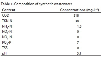
Experimental operation

Each biomass was cultured at room temperature (20.9 ± 0.6°C) in a 5 L (working volume) transparent glass bottle (18 cm diameter) with a cap (Fig. 1). Mixing was ensured by a magnetic stirrer at 300 r∙min⁻¹. Each reactor was operated as a sequencing batch reactor (SBR) without mechanical aeration. The SBR cycle consisted of a feeding phase (pump of 2.5 L of influent wastewater), a reaction phase, and a settling phase. A flexible plastic tube was used for extracting supernatant at the end of the settling phase and feeding the new synthetic wastewater at the beginning of the feeding phase. The volume exchange ratio was 50%. Feeding, reaction and settling phase durations were 1 h, 3.5 days and 1 h, respectively. The mean hydraulic residence time (HRT) was 7 days.

 

 

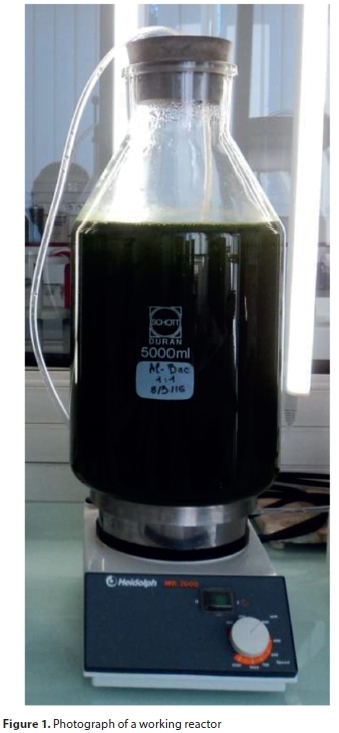
All reactors received the same illumination from 6 cool white light LEDs positioned 10 cm away from the reactors in vertical direction. Light intensity measured at the wall of reactor was 66 µEs⁻¹∙m⁻². Photoperiod was set up to 12 h light:12 h dark. Total culturing period was 1 month.

Analytical procedures

Dissolved oxygen concentration (DO) (WTW Inolab Oxi Level II Dissolved Oxygen Meter), pH and temperature (WTW pocket pH meter kits pH330) were measured daily at the central point of each reactor 5 h after illumination started and always before the settling phase. Due to this daily measurement frequency, it should be noticed that pH monitoring was performed once right before the feeding and then 1 day after.

Sampling for biomass analysis was performed twice per week at the end of each reaction phase. 100 mL of the well-mixed solution was sampled, right before the settling phase. Then the first 50 mL of this volume were filtered using 1.2 µm glass fibre filter (FILTRES RS) and used for TSS content determination (AFNOR NF T 90−105, 1997) The remaining 50 mL were filtered using 0.45 µm cellulose nitrate filter paper (Merck Millipore Ltd.) in dark conditions. The filter paper with suspension was then covered by aluminium paper, labelled and frozen before being analysed for total Chlorophyll _a (Chl-_a) content (AFNOR NF T 90−117, 1999).

The growth curves of TSS and Chl-_a were fitted using linear regression in order to compare the global growth rates between the experiments. Standard error was used to evaluate the variances of the fitted values and observed values of the biomass or Chl-_a growth rates (Crawley, 2012).

Sampling for nutrient content was performed daily including the same days as biomass sampling. Nutrient content was assessed in both input synthetic wastewater and supernatant effluent. At the beginning of each feeding phase, 300 mL of suspension was collected and filtered through sterile membrane (0.45 µm, filtraTECH) and frozen until analysis (within 1 month) of phosphorus (PO4-P) (ISO 6878:2004, 2004), nitrite nitrogen (NO2-N) (ISO 6777:1984, 1984), nitrate nitrogen (NO3-N) (ISO 7890-3:1988, 1988) and ammonium nitrogen (NH4-N) ((ISO 5664:1984, 1984)). Another unfiltered 100 mL sample was collected and used to analyse total Kjeldahl nitrogen (TKN-N) (ISO 5663:1984, 1984) and chemical oxygen demand (COD) (ISO 15705:2002, 2002).

Data analysis

Data collected were analysed by one-way analysis of variance (one-way ANOVA) with 95% confidence interval to assess if there was a statistical difference between the results for these systems. If a significant difference was detected, Holm tests were used to determine which pair of systems had a statistical difference at a 95% confidence interval. In addition, Welch test with 95% confidence interval was used to compare data representing different growing phases of each reactor. Data analysis was performed using R software (version 3.3.1 (2016-06−21)). Standard error was used to indicate the deviation from the mean with small sample size (_n < 30).

 

RESULTS AND DISCUSSION

Dynamics of dissolved oxygen and pH

The dynamics of algal-bacterial processes can be evaluated by assessing dissolved oxygen (DO) and pH variations. DO concentration is mainly governed by photosynthetic (oxygen production) and oxidative (oxygen uptake) activities of algae and bacteria, respectively (Muñoz and Guieysse, 2006). Via photosynthesis, algae consume inorganic carbon (HCO₃^-, CO₂) leading to an increase of pH in solution (Richmond, 2004; Park et al., 2010; Sutherland et al., 2015) while nitrification releases protons leading to pH decrease. These parameters were measured daily in each reactor to evaluate algal-bacterial processes during feeding and reaction phases (Figs 2 and 3).

 

 

 

 

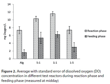
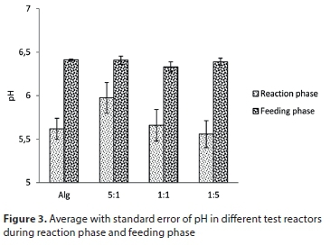
As expected, the feeding phase resulted in higher bacterial activity (heterotrophic growth and nitrification) because a high amount of dissolved organic matter and nutrients was available as substrate. For each reactor, this led to faster DO consumption and a decrease in its concentration: DO measured in the reaction phase was always higher than that in the feeding phase (_p < 0.05). Then, during the reaction phase, bacterial activity slowed down and O₂ release by algae led to O₂ increase in the medium.

The control reactor (algae only) and reactor with 1:5 algae/activated sludge inoculation ratio had similar DO content (_p > 0.05). This was also the case between reactors with 1:1 and 5:1 algae/activated sludge ratios (_p > 0.05). However, DO contents recorded in reactors with 1:1 and 5:1 algae/activated sludge ratios were higher than the control and 1:5 reactors (_p < 0.05). These results are in agreement with Chl-_a and TSS data (Figs 4 and 5) that showed that addition of activated sludge enhanced algal growth but that adding too much activated sludge leads to disturbances in algal growth.

 

 

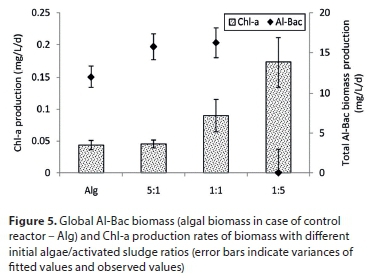
The pH level in an algal bacterial reactor is the consequence of algal productivity, algal/bacterial respiration, the alkalinity and ionic equilibriums, and autotrophic and heterotrophic microbial activities such as nitrification (Park et al., 2010).

Surprisingly, pH measured in the reaction phase was always lower than the pH measured in the feeding phase (Fig. 3), which was statistically proved by the Welch test with 95% confidence interval (_p < 0.05). However, one-way ANOVA with 95% confidence interval indicated that there is no significant difference between pH measured during the reaction phase of the four studied systems (_p > 0.05). The same conclusion was reached for pH in the feeding phase of all reactors (_p > 0.05).

Concerning pH, the observed values are globally acidic. Furthermore, photosynthesis during the reaction is supposed to make pH increase. However, the opposite trend was observed. Several causes can explain these unexpected trends:

•The prepared synthetic wastewater had a low pH (Table 1); this can explain the generally low pH level obtained during the entire experiment.

•The high pH increase (around one pH unit) between reaction and feeding phase indicated intensive photosynthetic activity following a feeding event (pH measurement was performed one day after).

•The decrease observed in the remaining days is mainly due to the nitrification process which acidifies the medium. This is consistent with Su et al. (2011) who observed a slight decrease in pH level over the first 5 days of each batch.

The fact that the nitrification process impact only appears after a few days is linked to the slower kinetics associated with this process: the maximum growth rates have been reported to be 1.3 d⁻¹ and 0.63 d⁻¹ at 20°C for algae and ammonia-oxidizing bacteria, respectively (Solimeno et al., 2017). Also, according to the stoichiometry of these biochemical reactions (Solimeno et al., 2017), the observed oxidation of around 25% of the nitrogen contained in the synthetic wastewater (see below) leads to the release of 1.35 meq H⁺∙L⁻¹ of protons (2 meq per mmol of N-NH₄⁺) while the maximum observed growth of algae (20 mg∙L⁻¹∙d⁻¹) leads to the release of 0.6 meq alkalinity∙L⁻¹. It should also be mentioned that the synthetic wastewater used had very low alkalinity, making it very sensitive to proton release. These low pH values could exert toxicity and/or inhibition effects on the biomass. However, the use of synthetic wastewater in this study could have played a role in avoiding these types of effects.

These results indicate that nitrification plays a significant role in TKN removal in these reactors.

Biomass growth

The growth of total Al-Bac biomass during the experimental period was estimated by TSS measurements. Since dissolved organic matter and nutrients were the only supplement provided for each reactor, any increase in total suspended solids inside the reactor was considered as a gain in biomass. Besides the total Al-Bac biomass, the global production of Chl-_a in each reactor during the experimental period, which is related to the increase of algae inside Al-Bac biomass (Park and Craggs, 2010), was also monitored (Fig. 4). TSS and Chl-_a concentrations increased almost linearly. The slopes of TSS and Chl-_a concentrations vs. time were used to derive the production rates displayed in Fig. 5.

After 1 month of experiments, all reactors showed a gain in biomass except the reactor with inoculation ratio of 1:5. The biomass growth rate in the reactor with only algae was lower than the ones inoculated with both algae and activated sludge (5:1 and 1:1). However, there was nearly no differences between growth rate of Al-Bac biomass 5:1 and 1:1. This result suggests that inoculation with both algae and activated sludge increases the production of Al-Bac biomass in comparison with only algae, but that an excessive amount of activated sludge added could decrease the growth of the biomass. A similar result was reported by Su et al. (2012b): with too much activated sludge added, the total algal-bacterial biomass increase at the end of the test was not as high as for other biomasses with lower activated sludge added. Disturbances in Al-Bac biomass growth could originate from the complex interactions between algae and bacteria in activated sludge (Cole, 1982; Kouzuma and Watanabe, 2015). Besides synergistic interactions resulting in fostering the growth of both algae and bacteria, there are antagonistic interactions between these organisms. These interactions, however, are numerous and depend on the species of algae and bacteria, growing states, and environmental conditions (Grossart and Simon, 2007).

In addition, the production rates of Chl-_a in reactors with 1:1 and 1:5 ratios were higher than the control reactor with only algae, indicating an acceleration of algal growth with the addition of activated sludge. However, there was no difference between Chl-_a production between Al-Bac biomass with 5:1 ratio and the control. This result is in good agreement with the conclusion reached by Roudsari et al. (2014), who observed that addition of activated sludge to up to 40% of the total biomass speeded up algal growth.

In comparison with literature, biomass volumetric production achieved in this study (below 20 mg∙L⁻¹∙d⁻¹⁾ could be considered to be rather low (Mata et al., 2010; Park et al., 2010). Su et al. (2011) cultivated an algae/activated sludge biomass in a batch reactor and reported a volumetric productivity of 38.8 mg∙L⁻¹∙d⁻¹. Van Den Hende et al. (2011) observed a mean value of 181 mg∙L⁻¹∙d⁻¹of algae/activated sludge biomass production in a reactor with flue gas supplement. In addition, Park and Craggs (2010) reported an algal-bacterial biomass volumetric production of 100 mg∙L⁻¹∙d⁻¹ obtained in an outdoor pilot high-rate algal pond wastewater treatment system with CO₂ addition. This may be explained by the low light intensity of 66 µEs⁻¹m⁻² applied in the present experiment. Indeed, algal growth and activity is enhanced under light intensity ranging from 200 to 400 µE s⁻¹m⁻² (Muñoz and Guieysse, 2006; Singh and Singh, 2015).

The increase of Al-Bac biomass and Chl-_a with 1:5 inoculation ratio suggests a significant replacement of the activated sludge biomass by algal biomass inside the Al-Bac biomass during the experiment. This illustrates the different dynamics of algal and bacterial growth in the system.

Biomass growth and settleability

Settling efficiency was evaluated by measuring supernatant TSS and Chl-_a concentrations after 1 h of gravitational settling. This reflects both wastewater treatment efficiency in terms of TSS and the possibility of efficiently harvesting the biomass.

All reactors provided good Chl-_a and Al-Bac biomass settling efficiencies (Table 2). This indicates good bio-flocculation between algae and activated sludge, as was observed in other studies (Gutzeit et al., 2005; Su et al., 2012b). Surprisingly, the control reactor with only algae also showed similar settling efficiency. This result differs from other studies which reported lower biomass settling efficiency of algae alone (Su et al., 2012b). The settling velocity of microalgal suspensions can differ greatly depending on culturing conditions (Gutiérrez et al., 2016). Several factors are involved, including long SRT (30 days) (Valigore et al., 2012), the dynamics of algae species (Su et al., 2012a) or pH (Vandamme et al., 2014). However, pH-induced flocculation is unlikely in the present study as pH was quite low (Fig. 3). In fact, the most probable factor explaining this observation is granulation as this was recently observed in SBRs (Liu et al., 2017; Cai et al., 2019). Indeed, the experimental conditions applied in this study may have selected for fast-settling biomass.

 

 

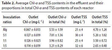
Nutrient removal efficiency

Similar effluent concentrations were recorded for all reactors (Table 3). The average COD removal efficiencies were 82±2, 79±2, 81±2 and 79±2% for the reactors with only algae, 5:1, 1:1 and 1:5 algae/activated sludge inoculation ratios, respectively. As there was significant COD removal in the control reactor with only algae, it does mean that bacteria growth occurred to some extent even without activated sludge inoculation. In comparison with other algal-bacterial biomass studies, COD removal efficiencies obtained in this study were at a good level (Gutzeit et al., 2005; Medina and Neis, 2007; Su et al., 2012b; Roudsari et al., 2014). However, phosphorus removal was not as high, with removal efficiencies of 30±5, 37±5, 33±3 and 15±11% for reactors with only algae, 5:1, 1:1 and 1:5 ratios, respectively.

 

 

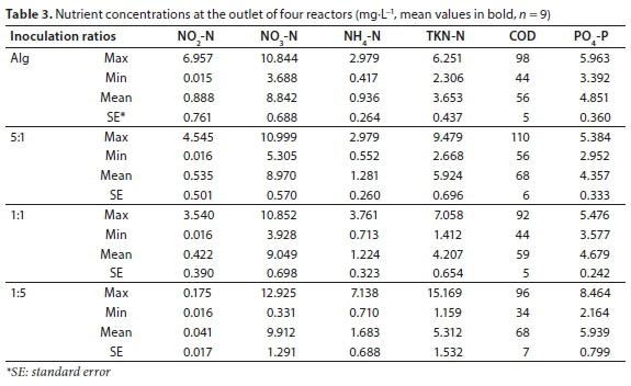
TKN-N removal ranged from 86 to 90%. Moreover, low NH₄-N and NO₂-N concentrations were measured in the effluent. Nitrification was therefore occurring to a large extent in all reactors, which is not in agreement with other algal-bacterial biomass studies (Gutzeit et al., 2005; Van Den Hende et al., 2011; Su et al., 2012b). Considering the NO₃-N concentrations, the total nitrogen removal efficiencies were 65±1, 61±2, 64±2, 61±3% for the reactors with only algae, 5:1, 1:1 and 1:5 algae/activated sludge inoculation ratios, respectively.

Nutrient removal efficiencies were similar between all tested reactors, which is not in agreement with other reports where different inoculation ratios induced varying efficiencies (Su et al., 2012b; Roudsari et al., 2014). Roudsari et al. (2014) conducted a 6-day batch experiment and concluded that a higher proportion of activated sludge improved COD removal while a higher proportion of algae improved ammonium nitrogen removal. The reason for these differences may derive from the long hydraulic and solids retention times (HRT = 7 days, SRT = 30 days) applied in the current experiment (García et al., 2000, 2002; Matamoros et al., 2015; Sutherland et al., 2015).

It is also important to note that the algal biomass inoculated in the control reactor was not pure culture, and thus bacteria, even in small amounts, were expected. Therefore, synthetic wastewater fed to the control reactor may stimulate bacterial growth. Thus, in this study, long HRT and SRT, as well as readily degradable organic matter, provide conditions that can promote the growth of this small amount of bacteria, even in the control reactor (Su et al., 2012b). Consequently, nitrification and heterotrophic growth of bacteria were also observed in this reactor.

The only exception was noted for phosphorus removal efficiency of Al-Bac biomass 1:5 reactor, where the removal efficiency varied widely (15±11%). This instability may originate from the high amount of activated sludge inoculated.

Final choice of optimal inoculation ratio

Results of this study showed an improvement in DO concentration in solution when an appropriate amount of activated sludge is added (1:1 and 5:1 algae/sludge ratios). In comparison, Al-Bac 5:1 had good total biomass growth, and good algal activity and nutrient removal efficiency. Nevertheless, it displayed a low algal growth rate similar the control reactor with only algal inoculum. Finally, Al-Bac 1:1 showed the best improvement in terms of total biomass, algal biomass growth and algal activity. A long-term study with a larger scale system is required to understand more about the dynamics between algae and bacteria. With these considerations, Al-Bac biomass with 1:1 inoculation ratio should be chosen for applying in a pilot culturing system for wastewater treatment and biomass production.

 

CONCLUSIONS

In this study, sequencing batch reactors were used to cultivate Al-Bac biomass with different algae/sludge inoculation ratios. In order to compare algal growth, initial algal biomass was similar in every test. DO concentration and Chl-_a content in all reactors were used to evaluate algal activities, with high levels of DO and Chl-_a growth rate indicating good algal activities in the reactor. Local algal biomass showed good incorporation with bacterial biomass (activated sludge): better algal growth occurred with Al-Bac biomass than with only algae.

Several conclusions were drawn as follows:

•Adding activated sludge accelerated the growth of Al-Bac biomass although the addition of too much activated sludge may cause disturbance to the total biomass growth. Algal growth also increased with addition of activated sludge but a significant amount of sludge was required to observe a significant change.

•Biomass settling and nutrient removal efficiencies were similar in every test including the control with only algae. Possible reasons include long hydraulic and solids retention times and occurrence of granulation.

•Among the three inoculation ratios evaluated, Al-Bac biomass with 1:1 inoculation ratio showed the best enhancement in total biomass, algal biomass growth, and algal activities.

 

REFERENCES

AFNOR NF T 90−105 (1997) Qualité de l'eau - Dosage des matières en suspension - Méthode par centrifugation. 1997.         [ Links ]

AFNOR NF T 90−117 (1999) Qualité de l'eau - Dosage de la chlorophylle a et d'un indice phéopigments - Méthode par spectrométrie d'absorption moléculaire. 1999.         [ Links ]

CAI W, ZHAO Z, LI D, LEI Z, ZHANG Z and LEE D-J (2019) Algae granulation for nutrients uptake and algae harvesting during wastewater treatment. Chemosphere 214 55-59. https://doi.org/10.1016/j.chemosphere.2018.09.107        [ Links ]

CHRISTENSON L and SIMS R (2011) Production and harvesting of microalgae for wastewater treatment biofuels and bioproducts. Biotechnol. Adv. 29 (6) 686-702. https://doi.org/10.1016/j.biotechadv.2011.05.015        [ Links ]

COLE JJ (1982) Interactions between bacteria and algae in aquatic ecosystems. Annu. Rev. Ecol. Syst. 13 (1) 291-314. https://doi.org/10.1146/annurev.es.13.110182.001451        [ Links ]

CRAGGS R, PARK J, SUTHERLAND D and HEUBECK S (2015) Economic construction and operation of hectare-scale wastewater treatment enhanced pond systems. J. Appl. Phycol. 27 (5) 1913-1922. https://doi.org/10.1007/s10811-015-0658-6        [ Links ]

CRAWLEY MJ (2012) The R Book (2^nd edn). Wiley-Blackwell, Chichester. 1076 pp.         [ Links ]

GARCÍA J., MUJERIEGO R and HERNANDEZ-MARINE M (2000) High rate algal pond operating strategies for urban wastewater nitrogen removal. J. Appl. Phycol. 12 (3-5) 331-339. https://doi.org/10.1023/A:1008146421368        [ Links ]

GARCÍA J, HERNÁNDEZ-MARINÉ M and MUJERIEGO R (2002) Analysis of key variables controlling phosphorus removal in high rate oxidation ponds provided with clarifiers. Water SA 28 (1) p-55. https://doi.org/10.4314/wsa.v28i1.4868        [ Links ]

GROSSART H-P and SIMON M (2007) Interactions of planktonic algae and bacteria: effects on algal growth and organic matter dynamics. Aquat. Microb. Ecol. 47 (2) 163. https://doi.org/10.3354/ame047163        [ Links ]

GUTIÉRREZ R, FERRER I, UGGETTI E, ARNABAT C, SALVADÓ H and GARCÍA J (2016) Settling velocity distribution of microalgal biomass from urban wastewater treatment high rate algal ponds. Algal Res. 16 409-417. https://doi.org/10.1016/j.algal.2016.03.037        [ Links ]

GUTZEIT G, LORCH D, WEBER A, ENGELS M and NEIS U (2005) Bioflocculent algal-bacterial biomass improves low-cost wastewater treatment. Water Sci. Technol. 52 (12) 9-18. https://doi.org/10.2166/wst.2005.0415        [ Links ]

ISO 5663:1984 (1984) Water quality - Determination of Kjeldahl nitrogen - Method after mineralization with selenium. 1984. ISO, Geneva.         [ Links ]

ISO 5664:1984 (1984) Water quality - Determination of ammonium - Distillation and titration method. 1984. ISO, Geneva.         [ Links ]

ISO 6777:1984 (1984) Water quality - Determination of nitrite - Molecular absorption spectrometric method. 1984. ISO, Geneva.         [ Links ]

ISO 6878:2004 (2004) Water quality - Determination of phosphorus - Ammonium molybdate spectrometric method. 2004. ISO, Geneva.         [ Links ]

ISO 7890-3:1988 (1988) Water quality - Determination of nitrate - Part 3: Spectrometric method using sulfosalicylic acid. 1988. ISO, Geneva.         [ Links ]

ISO 15705:2002 (2002) Water quality - Determination of the chemical oxygen demand index (ST-COD) - Small-scale sealed-tube method. 2002. ISO, Geneva.         [ Links ]

KOUZUMA A and WATANABE K (2015) Exploring the potential of algae bacteria interactions. Curr. Opin. Biotechnol. 33 125-129. https://doi.org/10.1016/j.copbio.2015.02.007        [ Links ]

LIU L, FAN H, LIU Y, LIU C and HUANG X (2017) Development of algae-bacteria granular consortia in photo-sequencing batch reactor. Bioresour. Technol. 232 64-71. https://doi.org/10.1016/j.biortech.2017.02.025        [ Links ]

MARA DD and PEARSON HW (1998) Design Manual for Waste Stabilization Ponds in Mediterranean Countries. Lagoon Technology International, Leeds, UK. 112 pp.         [ Links ]

MATA TM, MARTINS AA and CAETANO N (2010) Microalgae for biodiesel production and other applications: A review. Renew. Sustain. Energ. Rev. 14 (1) 217-232. https://doi.org/10.1016/j.rser.2009.07.020        [ Links ]

MATAMOROS V, GUTIÉRREZ R, FERRER I, GARCÍA J and BAYONA JM (2015) Capability of microalgae-based wastewater treatment systems to remove emerging organic contaminants: a pilot-scale study. J. Hazardous Mater. https://doi.org/10.1016/j.jhazmat.2015.02.002        [ Links ]

MEDINA M and NEIS U (2007) Symbiotic algal bacterial wastewater treatment: Effect of food to microorganism ratio and hydraulic retention time on the process performance. Water Sci. Technol. 55 (11) 165-71. https://doi.org/10.2166/wst.2007.351        [ Links ]

MUNOZ R and GUIEYSSE B (2006) Algal bacterial processes for the treatment of hazardous contaminants A review. Water Res. 40 (15) 2799-2815. https://doi.org/10.1016/j.watres.2006.06.011        [ Links ]

OECD (2001) OECD GUIDELINE FOR THE TESTING OF CHEMICALS. Simulation Test - Aerobic Sewage Treatment: 303 A: Activated Sludge Units - 303 B: Biofilms. 22. January 2001. OECD Publishing. https://doi.org/10.1787/9789264070424-en        [ Links ]

O'FLAHERTY E and GRAY NF (2013) A comparative analysis of the characteristics of a range of real and synthetic wastewaters. Environ. Sci. Pollut. Res. 20 (12) 8813-8830. https://doi.org/10.1007/s11356-013−1863-y        [ Links ]

OSWALD WJ and GOTAAS HB (1957) Photosynthesis in sewage treatment. Trans. Am. Soc. Civ. Eng. 122 (1) 73-97.         [ Links ]

PARK JBK and CRAGGS RJ (2010) Wastewater treatment and algal production in high rate algal ponds with carbon dioxide addition. Water Sci. Technol. 61 (3) 633. https://doi.org/10.2166/wst.2010.951        [ Links ]

PARK JBK, CRAGGS RJ and SHILTON AN (2010) Wastewater treatment high rate algal ponds for biofuel production. Bioresour. Technol. 102 (1) 35-42. https://doi.org/10.1016/j.biortech.2010.06.158        [ Links ]

PARK JBK, CRAGGS RJ and SHILTON AN (2011) Wastewater treatment high rate algal ponds for biofuel production. Bioresour. Technol. 102 (1) 35-42. https://doi.org/10.1016/j.biortech.2010.06.158        [ Links ]

PRAGYA N, PANDEY KK and SAHOO PK (2013) A review on harvesting, oil extraction and biofuels production technologies from microalgae. Renew. Sustain. Energ. Rev. 24 159-171. https://doi.org/10.1016/j.rser.2013.03.034        [ Links ]

RICHMOND A (2004) Handbook of Microalgal Culture: Biotechnology and Applied Phycology. Blackwell Publishing, Oxford, UK. 587 pp.         [ Links ]

ROUDSARI FP, MEHRNIA MR, ASADI A, MOAYEDI Z and RANJBAR R (2014) Effect of microalgae/activated sludge ratio on cooperative treatment of anaerobic effluent of municipal wastewater. Applied Biochemistry and Biotechnology 172 (1) 131-140. https://doi.org/10.1007/s12010-013-0480-z        [ Links ]

SALIM S, BOSMA R, VERMUË MH and WIJFFELS RH (2010) Harvesting of microalgae by bio-flocculation. J. Appl. Phycol. 23 (5) 849-855. https://doi.org/10.1007/s10811-010-9591-x        [ Links ]

SINGH SP and SINGH P (2015) Effect of temperature and light on the growth of algae species: A review. Renew. Sustain. Energ. Rev. 50 431-444. https://doi.org/10.1016/j.rser.2015.05.024        [ Links ]

SIRAJUNNISA AR and SURENDHIRAN D (2016) Algae - a quintessential and positive resource of bioethanol production: A comprehensive review. Renew. Sustain. Energ. Rev. 66 248-267. https://doi.org/10.1016/j.rser.2016.07.024        [ Links ]

SOLIMENO A, PARKER L, LUNDQUIST T and GARCÍA J (2017) Integral microalgae-bacteria model (BIO_ALGAE): Application to wastewater high rate algal ponds. Sci. Total Environ. 601-602 646-657. https://doi.org/10.1016/j.scitotenv.2017.05.215        [ Links ]

SU Y, MENNERICH A and URBAN B (2011) Municipal wastewater treatment and biomass accumulation with a wastewater-born and settleable algal-bacterial culture. Water Res. 45 (11) 3351-3358. https://doi.org/10.1016/j.watres.2011.03.046        [ Links ]

SU Y, MENNERICH A and URBAN B (2012a) Comparison of nutrient removal capacity and biomass settleability of four high-potential microalgal species. Bioresour. Technol. 124 157-162. https://doi.org/10.1016/j.biortech.2012.08.037        [ Links ]

SU Y, MENNERICH A and URBAN B (2012b) Synergistic cooperation between wastewater-born algae and activated sludge for wastewater treatment: Influence of algae and sludge inoculation ratios. Bioresour. Technol. 105 67-73. https://doi.org/10.1016/j.biortech.2011.11.113        [ Links ]

SUTHERLAND DL, HOWARD WILLIAMS C, TURNBULL MH, BROADY PA and CRAGGS RJ (2015) Enhancing microalgal photosynthesis and productivity in wastewater treatment high rate algal ponds for biofuel production. Bioresour. Technol. 184 (Advances in biofuels and chemicals from algae) 222-229. https://doi.org/10.1016/j.biortech.2014.10.074        [ Links ]

UDUMAN N, QI Y, DANQUAH MK, FORDE GM and HOADLEY A (2010) Dewatering of microalgal cultures: a major bottleneck to algae-based fuels. J. Renew. Sustain. Energ. 2 (1) 012701. https://doi.org/10.1063/1.3294480        [ Links ]

VALIGORE JM, GOSTOMSKI PA, WAREHAM DG and O'SULLIVAN AD (2012) Effects of hydraulic and solids retention times on productivity and settleability of microbial (microalgal-bacterial) biomass grown on primary treated wastewater as a biofuel feedstock. Water Res. 46 (9) 2957-2964. https://doi.org/10.1016/j.watres.2012.03.023        [ Links ]

VAN DEN HENDE S, BEELEN V, BORE G, BOON N and VERVAEREN H (2014) Upscaling aquaculture wastewater treatment by microalgal bacterial flocs From lab reactors to an outdoor raceway pond. Bioresour. Technol. 159 342-354. https://doi.org/10.1016/j.biortech.2014.02.113        [ Links ]

VAN DEN HENDE S, BEELEN V, JULIEN L, LEFOULON A, VANHOUCKE T, COOLSAET C, SONNENHOLZNER S, VERVAEREN H and ROUSSEAU DPL (2016) Technical potential of microalgal bacterial floc raceway ponds treating food-industry effluents while producing microalgal bacterial biomass: An outdoor pilot-scale study. Bioresour. Technol. 218 969-979. https://doi.org/10.1016/j.biortech.2016.07.065        [ Links ]

VAN DEN HENDE S, VERVAEREN H, DESMET S and BOON N (2011) Bioflocculation of microalgae and bacteria combined with flue gas to improve sewage treatment. New Biotechnol. 29 (1) 23-31. https://doi.org/10.1016/j.nbt.2011.04.009        [ Links ]

VANDAMME D, FOUBERT I and MUYLAERT K (2013) Flocculation as a low-cost method for harvesting microalgae for bulk biomass production. Trends Biotechnol. 31 (4) 233-239. https://doi.org/10.1016/j.tibtech.2012.12.005        [ Links ]

VANDAMME D, MUYLAERT K, FRAEYE I and FOUBERT I (2014) Floc characteristics of Chlorella vulgaris: Influence of flocculation mode and presence of organic matter. Bioresour. Technol. 151 383-387. https://doi.org/10.1016/j.biortech.2013.09.112        [ Links ]

VOLOSHIN RA, RODIONOVA MV, ZHARMUKHAMEDOV SK, NEJAT VEZIROGLU T and ALLAKHVERDIEV SI (2016) Review: Biofuel production from plant and algal biomass. Int. J. Hydrog. Energ. 41 (39) 17257-17273. https://doi.org/10.1016/j.ijhydene.2016.07.084        [ Links ]

 

 

Received 26 January 2018
Accepted in revised form 26 September 2019

 

 

* Corresponding author, email: julien.laurent@engees.unistra.fr

^rND^sCAI^nW^rND^sZHAO^nZ^rND^sLI^nD^rND^sLEI^nZ^rND^sZHANG^nZ^rND^sLEE^nD-J^rND^sCHRISTENSON^nL^rND^sSIMS^nR^rND^sCOLE^nJJ^rND^sCRAGGS^nR^rND^sPARK^nJ^rND^sSUTHERLAND^nD^rND^sHEUBECK^nS^rND^sGARCÍA^nJ^rND^sMUJERIEGO^nR^rND^sHERNANDEZ-MARINE^nM^rND^sGARCÍA^nJ^rND^sHERNÁNDEZ-MARINÉ^nM^rND^sMUJERIEGO^nR^rND^sGROSSART^nH-P^rND^sSIMON^nM^rND^sGUTIÉRREZ^nR^rND^sFERRER^nI^rND^sUGGETTI^nE^rND^sARNABAT^nC^rND^sSALVADÓ^nH^rND^sGARCÍA^nJ^rND^sGUTZEIT^nG^rND^sLORCH^nD^rND^sWEBER^nA^rND^sENGELS^nM^rND^sNEIS^nU^rND^sKOUZUMA^nA^rND^sWATANABE^nK^rND^sLIU^nL^rND^sFAN^nH^rND^sLIU^nY^rND^sLIU^nC^rND^sHUANG^nX^rND^sMATA^nTM^rND^sMARTINS^nAA^rND^sCAETANO^nN^rND^sMEDINA^nM^rND^sNEIS^nU^rND^sMUNOZ^nR^rND^sGUIEYSSE^nB^rND^sO'FLAHERTY^nE^rND^sGRAY^nNF^rND^sOSWALD^nWJ^rND^sGOTAAS^nHB^rND^sPARK^nJBK^rND^sCRAGGS^nRJ^rND^sPARK^nJBK^rND^sCRAGGS^nRJ^rND^sSHILTON^nAN^rND^sPARK^nJBK^rND^sCRAGGS^nRJ^rND^sSHILTON^nAN^rND^sPRAGYA^nN^rND^sPANDEY^nKK^rND^sSAHOO^nPK^rND^sROUDSARI^nFP^rND^sMEHRNIA^nMR^rND^sASADI^nA^rND^sMOAYEDI^nZ^rND^sRANJBAR^nR^rND^sSALIM^nS^rND^sBOSMA^nR^rND^sVERMUË^nMH^rND^sWIJFFELS^nRH^rND^sSINGH^nSP^rND^sSINGH^nP^rND^sSIRAJUNNISA^nAR^rND^sSURENDHIRAN^nD^rND^sSOLIMENO^nA^rND^sPARKER^nL^rND^sLUNDQUIST^nT^rND^sGARCÍA^nJ^rND^sSU^nY^rND^sMENNERICH^nA^rND^sURBAN^nB^rND^sSU^nY^rND^sMENNERICH^nA^rND^sURBAN^nB^rND^sSU^nY^rND^sMENNERICH^nA^rND^sURBAN^nB^rND^sSUTHERLAND^nDL^rND^sHOWARD WILLIAMS^nC^rND^sTURNBULL^nMH^rND^sBROADY^nPA^rND^sCRAGGS^nRJ^rND^sUDUMAN^nN^rND^sQI^nY^rND^sDANQUAH^nMK^rND^sFORDE^nGM^rND^sHOADLEY^nA^rND^sVALIGORE^nJM^rND^sGOSTOMSKI^nPA^rND^sWAREHAM^nDG^rND^sO'SULLIVAN^nAD^rND^sVAN DEN HENDE^nS^rND^sBEELEN^nV^rND^sBORE^nG^rND^sBOON^nN^rND^sVERVAEREN^nH^rND^sVAN DEN HENDE^nS^rND^sBEELEN^nV^rND^sJULIEN^nL^rND^sLEFOULON^nA^rND^sVANHOUCKE^nT^rND^sCOOLSAET^nC^rND^sSONNENHOLZNER^nS^rND^sVERVAEREN^nH^rND^sROUSSEAU^nDPL^rND^sVAN DEN HENDE^nS^rND^sVERVAEREN^nH^rND^sDESMET^nS^rND^sBOON^nN^rND^sVANDAMME^nD^rND^sFOUBERT^nI^rND^sMUYLAERT^nK^rND^sVANDAMME^nD^rND^sMUYLAERT^nK^rND^sFRAEYE^nI^rND^sFOUBERT^nI^rND^sVOLOSHIN^nRA^rND^sRODIONOVA^nMV^rND^sZHARMUKHAMEDOV^nSK^rND^sNEJAT VEZIROGLU^nT^rND^sALLAKHVERDIEV^nSI^rND^1A01^nWilza da Silva^sLopes^rND^1A01^nYsa Helena Diniz Morais de^sLuna^rND^1A02^nJose Tavares de^sSousa^rND^1A02^nWilton Silva^sLopes^rND^1A02^nValderi Duarte^sLeite^rND^1A01^nWilza da Silva^sLopes^rND^1A01^nYsa Helena Diniz Morais de^sLuna^rND^1A02^nJose Tavares de^sSousa^rND^1A02^nWilton Silva^sLopes^rND^1A02^nValderi Duarte^sLeite^rND^1A01^nWilza da Silva^sLopes^rND^1A01^nYsa Helena Diniz Morais de^sLuna^rND^1A02^nJose Tavares de^sSousa^rND^1A02^nWilton Silva^sLopes^rND^1A02^nValderi Duarte^sLeite

RESEARCH PAPERS

 

Evaluation of acidogenic sludge from anaerobic reactors running at low solids retention times to reduce sludge generation and enhance biogas production

 

 

Wilza da Silva Lopes^{I, *}; Ysa Helena Diniz Morais de Luna^I; Jose Tavares de Sousa^II; Wilton Silva Lopes^II; Valderi Duarte Leite^II

^IPrograma de Pós Graduação em Ciência e Tecnologia Ambiental, Universidade Estadual da Paraíba (UEPB),58429-500, Campina Grande, PB, Brazil
^IIDepartamento de Engenharia Sanitária e Ambiental, Universidade Estadual da Paraíba (UEPB), 58429-500, Campina Grande, PB, Brazil

 

 

---

ABSTRACT

Sludges generated in the biological processing of sewage are complex mixtures, the constituents of which pose risks to public health and the environment. Anaerobic digestion is considered the most sustainable option for treating sludge because it offers the possibility of generating biogas. The aim of this study was to compare the quantities, properties, biodegradabilities and biochemical methane potentials (BMP) of primary sludge (PS) generated by a primary decanter with acidogenic sludges produced by upflow anaerobic (UA) reactors operating at solids retention times (SRTs) of 2, 4, 6 and 8 days (Samples S2, S4, S6 and S8, respectively). Sludges from both pre-treatments were submitted to alkaline solubilization in order to determine the efficiency of the process in disrupting extracellular complexes. Based on the levels of total solids (TS) present, the primary decanter was found to generate higher quantities of excess sludge (yield of 3.1 gTS∙d⁻¹) than UA reactors operating at low SRTs (yields in the range 1.69 to 0.64 gTS∙d⁻¹). The concentrations of dissolved materials in PS and Samples S2 and S8 were considerably higher after alkaline solubilization, with respective increases of 8, 14 and 28-fold in dissolved organic carbon, 12, 20 and 40-fold in chemical oxygen demand, 25, 31 and 59-fold in proteins, and 17, 21 and 63-fold in carbohydrates. In addition, the BMP value for S8 was some 13% higher than that recorded for PS while the kinetic constant for gas production by S8 was 1.8-fold greater than that of PS. It is concluded that a pre-treatment combining anaerobic digestion at low SRT and alkaline solubilisation would lead to improved performance in subsequent stages of anaerobic digestion and, consequently, increased efficiency in biogas production.

Keywords: acidogenic sludge, sludge stabilisation, alkaline solubilisation, methanisation

---

 

 

INTRODUCTION

Sludge generated by the treatment of sewage is generally classified according to the stage of the process from which it originates. Thus, primary sludge arises from the gravitational sedimentation of suspended solids and organics, secondary sludge derives from the conversion of biodegradable material by microorganisms, and tertiary sludge originates from additional biological or chemical treatment.

Anaerobic digestion is considered the most sustainable option for the treatment of sludge because it is not only a relatively economical process but also produces biogas and a residue (biosolid) that can have green applications (Rani et al., 2012). In this context, decomposition of organic matter in the absence of free molecular oxygen affords some specific advantages such as the reduction of sludge volume by withdrawal of water, the transformation of highly biodegradable organic matter into relatively inert substances, the recovery of energy in the form of methane, and the generation of an end-product that can be disposed of in accordance with applicable legislation (Xu et al., 2014; Tchobanoglous et al., 2014).

The main steps involved in the anaerobic digestion of organic matter, namely hydrolysis, acidogenesis, acetogenesis and methanogenesis, require the balanced interaction of several groups of microorganisms in order to ensure rapid and successful degradation. The limiting step is hydrolysis in which insoluble substances, as well as high molecular weight compounds such as lipids, polysaccharides, proteins and nucleic acids, are broken down to soluble molecules that serve as substrates for the subsequent steps of the process (Gurje and Zehnder, 1983; Tchobanoglous et al., 2014). The hydrolytic step may also represent a pre-treatment method, since prior breakdown and solubilisation of sludge components accelerates anaerobic digestion and increases the efficiency of the process (Rani et al., 2012). A number of pre-treatment methods based on different operating strategies (i.e. biological, chemical, thermal, mechanical and combinations thereof) have been developed with the aim of improving the solubility of sludge solids (Chen et al., 2007; Cho et al., 2013; Bi et al., 2014; Tian et al., 2014; Xu et al., 2014; Sahinkaya, 2015).

Sludge derived from biological wastewater treatment contains two categories of organic complexes, namely soluble microbial products (SMP) and extracellular polymeric substances (EPS). The SMP comprise a pool of organic compounds that are weakly bound to cells or dissolved in solution, and may include humic acids, polysaccharides, proteins, amino acids, nucleic acids, organic acids, antibiotics, steroids, extracellular enzymes, structural components of cells and products of metabolism. The co-occurring EPS are the natural polymers secreted by microorganisms that play important roles in cell aggregation, cell adhesion, biofilm formation and, ultimately, protection against hostile environments (Sheng et al., 2010; Wang et al., 2014). Since EPS matrices are strongly attached to the cells, their disruption requires the application of powerful procedures such as alkaline solubilisation.

Upflow anaerobic (UA) reactors operating at a low solids retention time (SRT) generate less sludge than conventional primary decanters and could replace decanters in pre-treatment processes in order to minimise the volume of sludge to be treated. Hence, the aim of this study was to compare the quantities, properties, biodegradabilities and biochemical methane potentials (BMP) of primary sludge (PS) generated by a primary decanter with acidogenic sludges produced by UA reactors operating at SRTs of 2, 4, 6 and 8 days. Sludges from both pre-treatments were submitted to alkaline solubilization in order to determine the efficiency of the process in disrupting extracellular complexes.

 

METHODS

Pre-treatment of sanitary sewage

Two routes of pre-treatment of sanitary sewage were studied in parallel, as outlined in Figure 1, and the characteristics and energy potential of the sludges so-produced were compared.

 

 

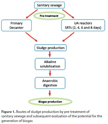
The sanitary sewage used in the experiment originated from the eastern interceptor of the Companhia de Água e Esgoto da Paraíba (CAGEPA; Campina Grande, PB, Brazil) and was characterized prior to treatment as follows: pH 7.62, total alkalinity 454.8 mgCaCO₃∙L⁻¹, total solids (TS) 820 mg∙L⁻¹, volatile suspended solids (VSS) 360 mg∙L⁻¹, total chemical oxygen demand (COD_T) 764 mg∙L⁻¹, soluble COD 272 mg∙L⁻¹, total phosphorus (TP) 14.5 mg∙L⁻¹, and total Kjeldahl nitrogen (TKN) 87.8 mg∙L⁻¹.

Acidogenic sludges were obtained from four UA reactors (each of volume 2 L) that were fed daily with sanitary sewage and operated simultaneously with hydraulic retention times (HRT) of 4 h, flow rates of 12 L∙day⁻¹ and SRTs of 2, 4, 6 or 8 days (S2, S4, S6 and S8 sludges, respectively). For sludge disposal, all of the reactor contents (mixed liquor) were withdrawn and, after homogenisation, quantities equivalent to ½, ¼, ¹�₆ and ⅛ of the total volume were removed for physicochemical analysis with the remainder being returned to the reactor to maintain SRTs of 2, 4, 6 and 8 days, respectively. Primary sludge was obtained by sedimentation of 12 L of sanitary sewage for 1 h. The supernatant was removed from the 1 L of thickened sewage so-formed, and the sediment that remained was characterized as PS.

Samples of sludges were characterized daily over a 2-month experimental period and excess sludge production of the primary decanter and UA reactors was calculated on the basis of the measured values of TS.

Physicochemical analyses of sludges

Viscosities of sludge samples were measured using a Q860M26 microprocessor-controlled rotational viscometer (Quimis, Diadema, SP, Brazil), while values of the specific resistance to filtration (SRF) were established according to methodology described by Almeida et al. (1991). Total dissolved solids (TDS), total volatile solids (TVS), total suspended solids (TSS), volatile dissolved solids (VDS), fixed dissolved solids (FDS), dissolved organic carbon (DOC), TS, VSS, COD_T, TKN and TP were determined following the methodologies recommended by the American Public Health Association (2012). Concentrations of SMP and EPS were assessed in terms of protein and carbohydrate content established according to the methods of Lowry et al. (1951) (as modified by Frølund et al., 1995) and Dubois et al. (1956), respectively. For this purpose, samples of sludge were centrifuged at 4°C for ١٥ min at 15 455 g and the supernatants were filtered through 0.45 μm glass fibre membranes and employed in the SMP assays, while the sediments were extracted with 0.05% NaCl solution for 30 min at 60°C (Li and Yang, 2007) and submitted to EPS assay.

Statistical analysis

Data were submitted to one-way analysis of variance (ANOVA) with post-hoc Tukey multiple comparison tests in order to detect significant differences (p < 0.05) between mean values of the parameters determined for the sludge samples. Based on the results of the statistical analysis, sludge samples PS, S2 and S8 were selected for further investigation as described below.

Alkaline solubilisation of sludges

The selected samples were submitted to alkaline solubilisation in triplicate in order to compare the degree of solubilisation of their constituents. Aliquots (100 mL) of sludges were adjusted to pH 12.0 with 1 M NaOH solution and maintained under constant agitation at 200 r∙min⁻¹ on a gyrotory shaker mixer model G-33 (New Brunswick Scientific, Edison, NJ, United Sates ) for 48 h at approximately 28°C (Monte et al., 2017). Treated samples were subsequently brought to neutral conditions (pH 7.0) by the addition of 1 M HCl and concentrations of carbohydrates, proteins, TDS, VDS, FDS, COD and DOC determined. The masses of NaOH and HCl required to adjust the pH values of sludge samples to those specified in the pre-treatment protocol were determined in a preliminary experiment in which 20 mL aliquots of each sample were titrated sequentially with 1M NaOH and 1M HCl solutions under constant monitoring of pH (Table 1).

 

 

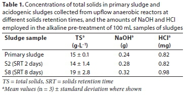
Determination of biochemical methane potential

Assessments of BMP were performed using 250 mL borosilicate flasks containing inoculum (from an upflow anaerobic sludge blanket reactor) and substrate sample (PS or S8 sludge) in the proportion of 2:1. The flasks were placed in an incubator at a constant temperature of 35±2°C (appropriate for mesophilic bacteria) with regular agitation. Assays were continued for 21 days, at which point the cumulative biogas curves had entered the plateau region (Angelidaki et al., 2009).

 

RESULTS AND DISCUSSION

Effect of low SRT on the chemical characteristics of acidogenic sludges

The mean values of solids, COD_T, TKN and TP, as determined from daily measurements of PS samples and on the accumulated levels in sludges collected during the acidogenic process in UA reactors operating at low SRTs, are shown at Table 2. The concentrations of TS and TSS in the sludges showed a general tendency to rise as SRT increased, even though the levels in S2 and S4 were similar. The overall pattern can be explained by the consumption of organic matter present in the sewage by metabolic processes of the microorganisms, in that the removal of organic matter from the effluent of the reactor and the quantity of sludge biomass produced were maximal at an SRT of 8 days. The volatile fraction accounted for the greater part (on average 75%) of the TS present in all of the sludge samples analysed. Regarding COD_T, the lowest concentration was observed in S2 while the highest was recorded in S8. TKN also tended to increase with increasing SRT, which may be explained by the assimilation of the nitrogen present in the sewage resulting from anabolism of the sludge biomass growing inside the reactors and by assimilation of nitrogen compounds by the EPS biofilm formed on the sludge flakes. No variations were detected in the concentrations of TP in any of the sludge samples, probably because all four reactors operated at low SRTs and the anaerobic process does not effectuate phosphorus removal.

Based on the TS values shown in Table 2, it is possible to estimate the amount of sludge generated in the primary decanter and the UA reactors. At a sewage flow of 12 L∙d⁻¹, the primary decanter produced 1L of PS with a TS concentration of 3.1 g∙L⁻¹, resulting in a yield of 3.1 g TS∙d⁻¹. Considering that 1/2, 1/4, 1/6 and 1/8 of the contents of the reactors S2, S4, S6 and S8, respectively, were removed for analysis, the corresponding amounts of excess sludge generated by the UA reactors would be 1.69, 0.82, 0.64 and 0.69 g TS∙d⁻¹.

Effect of low SRT on the biochemical composition and physical properties of acidogenic sludges

The concentration of proteins predominated over that of carbohydrates in the SMP and EPS fractions of all sludge samples analysed (Table 3), thereby corroborating the findings of Li and Yang (2007). With regard to SMP, the highest mean concentrations of proteins and carbohydrates were observed in PS and the lowest in S8 signifying that, for SRT > 2 days, the levels of SMP in the sludge decreased substantially with increasing SRT. Li and Yang (2007) also recorded higher SMP concentrations at lower SRTs, a finding that may be ascribed to the assimilation of soluble material by microorganisms present in the liquid fraction resulting in the development of cell aggregates that form part of the structure of the sludge. Since high concentrations of SMP can adversely affect the sedimentation and dewatering characteristics of sludge, an understanding of how factors such as SRT, HRT and organic load influence the production of SMP is important for improving the design and operation of wastewater treatment plants (Aquino et al., 2009; Kunacheva et al., 2017).

 

 

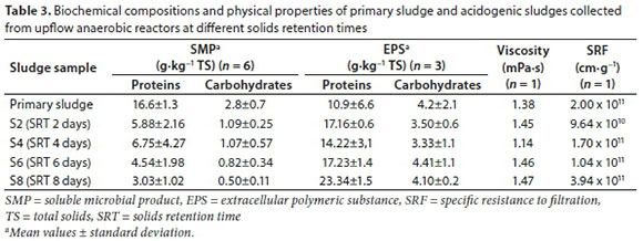
In the case of EPS, the highest mean concentration of proteins was observed in S8 and the lowest in PS (Table 3). On this basis, the levels of EPS in sludge would appear to show a tendency to rise with increasing SRT. On the other hand, the levels of carbohydrates in EPS showed relatively small fluctuations between sludge samples, a finding in accordance with the report of Li and Yang (2007) that the amount of EPS does not vary significantly with increasing SRT. According to Ye et al. (2011), the concentration of EPS in sludge depends on a number of variables, including the amount of residual water, level of nutrients, reactor configuration and SRT.

The viscosities of sludges S2, S6 and S8 were similar but showed slight rises with increasing SRT (Table 3). On the other hand, the viscosity of S4 was somewhat lower than that of the other sludges, reflecting the decreased concentration of EPS as indicated by the reduced protein and carbohydrate levels exhibited by this sample. Thus, our results suggest a direct relationship between viscosity and EPS concentration. A similar association can be observed between SRF and EPS, since the lowest resistance value was recorded with S2 and the highest with S8.

Aggregation of dispersed microorganisms leads to increased particle size, and this gives rise to denser flocs and promotes the incrementation of EPS. Moreover, dehydration of the sludge becomes more difficult with higher SRTs by virtue of the increases in SRF, EPS and viscosity (Feng et al., 2016). In the present study, the SRTs adopted were relatively low (maximum 8 days) and the elevated levels of EPS and viscosity observed did not appear to hinder sludge dewatering. Indeed, higher levels of EPS may be advantageous since the larger amount of organic matter present would allow higher biogas generation.

Solubilisation of acidogenic and primary sludges by alkaline pre-treatment

Since the mean values of most of the parameters determined for Sludges S2, S4 and S6 were not significantly different (Table 2), the SRT that was most applicable from the point of view of cost (namely, 2 days) was selected as representative of these samples for the alkaline solubilization test. After 48 h of alkaline pre-treatment, PS and sludge samples S2 and S8 presented elevated concentrations of dissolved materials with respective increases of 4.7, 3.9 and 5.7-fold in TDS, 5.7, 5.7 and 10-fold in VDS, and 4.3, 3.4 and 4.4-fold in FDS (Table 4).

The amounts of DOC in PS, S2 and S8 after alkaline solubilisation were, respectively, 8, 14 and 28-fold higher than those detected in the samples prior to the procedure (Table 4). It is important to note that, even though S2 had been generated with a very short SRT, the amount of solubilised material present in the sample after alkaline treatment was greater than that detected in solubilised PS. The levels of COD also rose appreciably after alkaline treatment with 12, 20 and 40-fold increases recorded in PS, S2 and S8, respectively. A number of researchers have reported significant enhancements in COD following alkaline solubilisation with recorded increases of 2-times (Cho et al., 2013), 17-times (Chen et al., 2007) and 100-times (Xu et al., 2014) the pre-treatment levels. Thus, alkaline solubilisation is an effective method of destroying cell matrices and increasing the concentration of soluble materials. Moreover, since the values of TDS, VDS, FDS, DOC and COD increased gradually from PS to S8, it would appear that the amount of soluble material produced by alkaline solubilisation is related directly to SRT.

The concentrations of dissolved proteins and carbohydrates increased considerably in PS, S2 and S8 following alkaline solubilisation, with respective gains of 25, 31 and 59-fold for proteins and 17, 21 and 63-fold for carbohydrates (Table 4). Previous studies of the effects of alkaline pre-treatment (pH 12) of sludges have revealed increases in the concentrations of proteins and carbohydrates, respectively, in the order of 9.4 and 7.8-fold (Chen et al., 2007), 2.8 and 1.4-fold (Cho et al., 2013), 3.0 and 2.8-fold (Xu et al., 2014) and 26.3 and 36.9-fold (Monte et al., 2017). Our results are in accord with earlier reports and demonstrate that alkaline solubilisation of acidogenic sludge is efficient in the disruption of EPS, thereby overcoming the limitations of the hydrolytic step of degradation and making available larger amounts of substrate for methanogenesis.

Samples of PS, S2 and S8 showed increased concentrations of dissolved TP and TKN following alkaline solubilisation (Table 4), although the respective gains (i.e. 1.5, 1.7 and 4.0-fold for TP and 2.9, 2.3 and 5.5-fold for TKN) were not as pronounced as those recorded for the other variables studied. Kim et al. (2003) also obtained low values for nitrogen and phosphorus using the alkaline solubilisation process, while Chen et al. (2007) reported that solubilisation at low pH values (4.0 to 5.0) was more effective in increasing the concentrations of these constituents. One explanation for this finding is that the activities of hydrolytic enzymes may be reduced at higher pH values.

Pre-treatment of sanitary sewage using a combination of UA digestion at low SRT and alkaline solubilisation affords a number of advantages considering that the process involves proven technologies that are simple to apply and control, and that the pH of the sludge can be raised using a wide range of low-cost materials such as limestone (CaCO₃), CaO, Ca(OH)₂, NaOH, Na₂CO₃ and ammonia. The disadvantages include the inclusion of a separate stage in the digestion process and the non-selectivity of the solubilisation stage.

Biogas production

The generation of biogas was evaluated with PS and with Sample S8 because sludge produced in a UA with an SRT of 8 days contained the highest concentrations of organic matter as indicated by the values of COD and EPS (Tables 2 and 3). As shown in Fig. 2, PS generated more biogas than S8 in the first 8 days, likely because the initial digestion process in S8 increased the lead-time for methanation since soluble materials present in the liquid fraction are first degraded and sludge flakes are formed. The volumes of biogas produced by PS and S8 were similar at Day 9, after which the production of biogas by S8 surpassed that of PS with both sludges reaching a constant rate at Day 16. According to the BMP values for PS and S8 (i.e. 56.8 and 64.1 NmL∙g⁻¹ VSS, respectively), the acidogenic sludge showed a 13% increase in biogas potential that could be explained by the incorporation of soluble material into the biomass, as demonstrated by the increase in EPS values. Kooijman et al. (2017) reported that the addition of flocculants during primary settling enhanced the removal of more readily degradable solids and increased the BMP of PS.

 

 

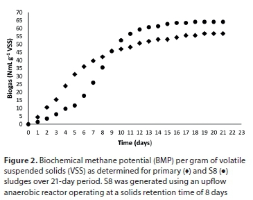
Although the difference in biogas production between PS and S8 was not remarkable, the increase observed with S8 would become more expressive during large-scale processing. More importantly, the values of the kinetic constants, derived from sludge biogas curves on the basis that biogas production obeys first-order kinetics, were established to be 0.09 d⁻¹ for PS and 0.165 d⁻¹ for S8. In this sense, the higher rate of conversion of organic matter obtained with S8 is significant because it implies that a shorter time would be required to stabilize the sludge in the reactor. From an engineering viewpoint, this finding is very relevant since it signifies that smaller digesters can be used in the treatment of such sludges with attendant reductions in processing costs.

 

CONCLUSIONS

The amount of solid material in sludges produced by four UA reactors running at a fixed HRT (4 h) with a 12 L∙day⁻¹ flow rate increased with SRTs within the range of 2 to 8 days. The level of EPS also increased with increasing SRT owing to the formation of cell aggregates with concomitant utilisation of soluble proteins and carbohydrates. The concentrations of TDS, VDS, FDS, DOC, COD, proteins and carbohydrates in the sludges increased after alkaline solubilisation according to the order S8 > S2 > PS. The results indicate that, in comparison with the primary decanter, UA reactors running at low SRTs produced less excess sludge, sludges with higher amounts of soluble materials and, consequently, higher biogas potential. In addition, alkaline solubilization of the sludge should lead to better performance in the last stages of anaerobic digestion with greater efficiency in biogas generation.

 

ACKNOWLEDGEMENTS

The authors thank Coordenação de Aperfeiçoamento de Pessoal de Nível Superior (CAPES), Conselho Nacional de Desenvolvimento Científico e Tecnológico (CNPq) and Financiadora de Estudos e Projetos (FINEP) for financial support.

 

REFERENCES

ALMEIDA GN, GONÇALVES MC and GUIMARÃES SAZ (1991) Utilização do teste de resistência específica na operação de filtros prensa. Revista DAE 160 20-26. http://revistadae.com.br/artigos/artigo_edicao_160_n_115.pdf        [ Links ]

AMERICAN PUBLIC HEALTH ASSOCIATION (2012) Standard Methods for the Examination of Water and Wastewater (22^nd edn). APHA, Washington.         [ Links ]

ANGELIDAKI I, ALVES M, BOLZONELLA D, BORZACCONI L, CAMPOS JL, GUWY AJ, KALYUZHNYI S, JENICEK P and VAN LIER JB (2009) Defining the biomethane potential (BMP) of solid organic wastes and energy crops: a proposed protocol for batch assays. Water Sci. Technol. 59 927-934. https://doi.org/10.2166/wst.2009.040        [ Links ]

AQUINO SF, GLORIA RM, SILVA SQ and CHERNICHARO CA (2009) Quantification of the inert chemical oxygen demand of raw wastewater and evaluation of soluble microbial product production in demo-scale upflow anaerobic sludge blanket reactors under different operational conditions. Water Environ. 81 608-616. https://doi.org/10.2175/106143008X370386        [ Links ]

BI W, LI Y and HU Y (2014) Recovery of phosphorus and nitrogen from alkaline hydrolysis supernatant of excess sludge by magnesium ammonium phosphate. Bioresour. Technol. 166 1-8. https://doi.org/10.1016/j.biortech.2014.04.092        [ Links ]

CHEN Y, JIANG S, YUAN H, ZHOU Q and GU G (2007) Hydrolysis and acidification of waste activated sludge at different pHs. Water Res. 41 683-689. https://doi.org/10.1016/j.watres.2006.07.030        [ Links ]

CHO HU, PARK SK, HA JH and PARK JM (2013) An innovative sewage sludge reduction by using a combined mesophilic anaerobic and thermophilic aerobic process with thermal-alkaline treatment and sludge recirculation. J. Environ. Manage. 129 274-282. https://doi.org/10.1016/j.jenvman.2013.07.009        [ Links ]

DUBOIS M, GILLES KA, HAMILTON JK, REBERS PA and SMITH F (1956) Colorimetric method for determination of sugars and related substances. Anal. Chem. 28 350-356. https://doi.org/10.1021/ac60111a017        [ Links ]

FENG X, TANG B, BIN L, SONG H, HUANG S, FU F, DING J, CHEN C and YU C (2016). Rheological behavior of the sludge in a long-running anaerobic digestor: Essential factors to optimize the operation. Biochem. Eng. J. 114 147-154. https://doi.org/10.1016/j.bej.2016.06.022        [ Links ]

FRØLUND B, GRIEBE T and NIELSEN PH (1995) Enzymatic activity in the activated-sludge floc matrix. Appl. Microbiol. Biotechnol. 43 755-761. https://doi.org/10.1007/BF00164784        [ Links ]

GURJE W and ZEHNDER AJB (1983) Conversion processes in anaerobic digestion. Water Sci. Technol. 15 127-167. https://doi.org/10.2166/wst.1983.0164        [ Links ]

KIM J, PARK C, KIM T-H, LEE M, KIM S, KIM S-W and LEE J (2003) Effects of various pretreatments for enhanced anaerobic digestion with waste activated sludge. J. Biosci. Bioeng. 95 271-275. https://doi.org/10.1016/S1389−1723(03)80028-2        [ Links ]

KOOIJMAN G, DE KREUK MK and VAN LIER JB (2017) Influence of chemically enhanced primary treatment on anaerobic digestion and dewaterability of waste sludge. Water Sci. Technol. 76 1629-1639. https://doi.org/10.2166/wst.2017.314        [ Links ]

KUNACHEVA C, SOH YNA and STUCKEY DC (2017) Effect of feed pH on reactor performance and production of soluble microbial products (SMPs) in a submerged anaerobic membrane bioreactor. Chem. Eng. J. 320 135-143. https://doi.org/10.1016/j.cej.2017.03.018        [ Links ]

LI XY and YANG SF (2007) Influence of loosely bound extracellular polymeric substances (EPS) on the flocculation, sedimentation and dewaterability of activated sludge. Water Res. 41 1022-1030. https://doi.org/10.1016/j.watres.2006.06.037        [ Links ]

LOWRY OH, ROSEBROUGH NJ, FARR AL and RANDALL RJ (1951) Protein measurement with the Folin phenol reagent. J. Biol. Chem. 193 265-275. http://www.jbc.org/content/193/1/265.short        [ Links ]

MONTE FP, BRITO ALM, LOPES WS and CEBALLOS BSO (2017) Aumento da produção de biogás (metano) a partir da solubilização de lodos de esgotos. In: Costa One GM and Albuquerque HN (eds). Saúde e Meio Ambiente: Os Desafios da Interdisciplinaridade nos Ciclos da Vida Humana. Instituto Bioeducação, Campina Grande. 276-294. http://cinasama.com.br/upload/160217040814257614.pdf        [ Links ]

RANI R U, KALIAPPAN S, KUMAR S A and BANU JR (2012) Combined treatment of alkaline and disperser for improving solubilization and anaerobic biodegradability of dairy waste activated sludge. Bioresour. Technol. 126 107-116. https://doi.org/10.1016/j.biortech.2012.09.027        [ Links ]

SAHINKAYA S (2015) Disintegration of municipal waste activated sludge by simultaneous combination of acid and ultrasonic pretreatment. Process Saf. Environ. 93 201-205. https://doi.org/10.1016/j.psep.2014.04.002        [ Links ]

SHENG G-P, YU H-Q and LIX-Y (2010) Extracellular polymeric substances (EPS) of microbial aggregates in biological wastewater treatment systems: A review. Biotechnol. Adv. 28 882-894. https://doi.org/10.1016/j.biotechadv.2010.08.001        [ Links ]

TCHOBANOGLOUS G, BURTON FL and STENSEL HD (2014) Wastewater Engineering: Treatment and Resource Recovery (5^th edn). McGraw Hill, New York.         [ Links ]

TIAN X, WANG C, TRZCINSKI A P, LIN L and NG WJ (2014) Insights on the solubilization products after combined alkaline and ultrasonic pre-treatment of sewage sludge. J. Environ. Sci. 29 97-105. https://doi.org/10.1016/j.jes.2014.07.024        [ Links ]

WANG Z, MA J, TANG CY, KIMURA K, WANG Q and HAN X (2014) Membrane cleaning in membrane bioreactors: A review. J. Membrane Sci. 468 276-307. https://doi.org/10.1016/j.memsci.2014.05.060        [ Links ]

XU J, YUAN H, LIN J and YUAN W (2014) Evaluation of thermal, thermal-alkaline, alkaline and electrochemical pretreatments on sludge to enhance anaerobic biogas production. J. Taiwan Inst. Chem. Eng. 45 2531-2536. https://doi.org/10.1016/j.jtice.2014.05.029        [ Links ]

YE F, PENG G and LI Y (2011) Influences of influent carbon source on extracellular polymeric substances (EPS) and physicochemical properties of activated sludge. Chemosphere 84 1250-1255. https://doi.org/10.1016/j.chemosphere.2011.05.004        [ Links ]

 

 

Received 2 April 2018
Accepted in revised form 23 September 2019

 

 

* Corresponding author, email: wilzasilvalopes@hotmail.com

^rND^sALMEIDA^nGN^rND^sGONÇALVES^nMC^rND^sGUIMARÃES^nSAZ^rND^sANGELIDAKI^nI^rND^sALVES^nM^rND^sBOLZONELLA^nD^rND^sBORZACCONI^nL^rND^sCAMPOS^nJL^rND^sGUWY^nAJ^rND^sKALYUZHNYI^nS^rND^sJENICEK^nP^rND^sVAN LIER^nJB^rND^sAQUINO^nSF^rND^sGLORIA^nRM^rND^sSILVA^nSQ^rND^sCHERNICHARO^nCA^rND^sBI^nW^rND^sLI^nY^rND^sHU^nY^rND^sCHEN^nY^rND^sJIANG^nS^rND^sYUAN^nH^rND^sZHOU^nQ^rND^sGU^nG^rND^sCHO^nHU^rND^sPARK^nSK^rND^sHA^nJH^rND^sPARK^nJM^rND^sDUBOIS^nM^rND^sGILLES^nKA^rND^sHAMILTON^nJK^rND^sREBERS^nPA^rND^sSMITH^nF^rND^sFENG^nX^rND^sTANG^nB^rND^sBIN^nL^rND^sSONG^nH^rND^sHUANG^nS^rND^sFU^nF^rND^sDING^nJ^rND^sCHEN^nC^rND^sYU^nC^rND^sFRØLUND^nB^rND^sGRIEBE^nT^rND^sNIELSEN^nPH^rND^sGURJE^nW^rND^sZEHNDER^nAJB^rND^sKIM^nJ^rND^sPARK^nC^rND^sKIM^nT-H^rND^sLEE^nM^rND^sKIM^nS^rND^sKIM^nS-W^rND^sLEE^nJ^rND^sKOOIJMAN^nG^rND^sDE KREUK^nMK^rND^sVAN LIER^nJB^rND^sKUNACHEVA^nC^rND^sSOH^nYNA^rND^sSTUCKEY^nDC^rND^sLI^nXY^rND^sYANG^nSF^rND^sLOWRY^nOH^rND^sROSEBROUGH^nNJ^rND^sFARR^nAL^rND^sRANDALL^nRJ^rND^sMONTE^nFP^rND^sBRITO^nALM^rND^sLOPES^nWS^rND^sCEBALLOS^nBSO^rND^sRANI R^nU^rND^sKALIAPPAN^nS^rND^sKUMAR S^nA^rND^sBANU^nJR^rND^sSAHINKAYA^nS^rND^sSHENG^nG-P^rND^sYU^nH-Q^rND^sLIX-Y^rND^sTIAN^nX^rND^sWANG^nC^rND^sTRZCINSKI A^nP^rND^sLIN^nL^rND^sNG^nWJ^rND^sWANG^nZ^rND^sMA^nJ^rND^sTANG^nCY^rND^sKIMURA^nK^rND^sWANG^nQ^rND^sHAN^nX^rND^sXU^nJ^rND^sYUAN^nH^rND^sLIN^nJ^rND^sYUAN^nW^rND^sYE^nF^rND^sPENG^nG^rND^sLI^nY

CANTRELL KJ, KAPLAN DI and WIETSMA TW (1995) Zero-valent iron for the in situ remediation of selected metals in groundwater. J. Hazardous Mater. 42 (2) 201-212. https://doi.org/10.1016/0304-3894(95)00016-n        [ Links ]

CHANDRAPPA AK and BILIGIRI KP (2016) Pervious concrete as a sustainable pavement material - research findings and future prospects: A state-of-the-art review. Constr. Build. Mater. 111 262-274. https://doi.org/10.1016/j.conbuildmat.2016.02.054        [ Links ]

CUNDY AB, HOPKINSON L and WHITBY RLD (2008) Use of iron-based technologies in contaminated land and groundwater remediation: A review. Sci. Total Environ. 400 42-51.         [ Links ]

EKOLU SO and BITANDI LK (2018) Prediction of longevities of ZVI and pervious concrete reactive barriers using the transport simulation model. J. Environ. Eng. 144 (9) https://doi.org/10.1061/(ASCE)EE.1943-7870.0001402.         [ Links ]

EKOLU SO, AZENE FZ and DIOP S (2014a) A concrete reactive barrier for acid mine drainage treatment. Water Manage. 167 (7) 373-380. https://doi.org/10.1680/wama.13.00035        [ Links ]

EKOLU SO, DIOP S and AZENE F (2014b) Bottom ash and fly ash wastes as alkalinising reagents for acid mine drainage. Proceedings of the International Conference on Construction Materials and Structures (ICCMATS), 24-26 November 2014, Johannesburg, South Africa. 1427-1435.         [ Links ]

EKOLU SO, DIOP S and AZENE F (2016a) Properties of pervious concrete for hydrological applications. Concrete Beton 144 18-25.         [ Links ]

EKOLU SO, DIOP S, AZENE F and MKHIZE N (2016b) Disintegration of concrete construction induced by acid mine drainage attack. J. S. Afr. Inst. Civ. Eng. 58 (1) 34-42. http://dx.doi.org/10.17159/2309-8775/2016/v58n1a4        [ Links ]

FERNANDO WAM, ILANKOON IMSK, SYED TH and YELLISHETTY M (2018) Challenges and opportunities in the removal of sulphate ions in contaminated mine water: A review. Miner. Eng. 117 74-90. https://doi.org/10.1016/j.mineng.2017.12.004        [ Links ]

FITZPATRICK RW (2003) Overview of acid sulfate soil properties, environmental hazards, risk mapping and policy development in Australia. In: Roach IC (ed.) Advances in Regolith. RC LEME, Adelaide. 22-125.         [ Links ]

FORD KL (2003) Passive treatment systems for acid mine drainage. Technical Note 409, Bureau of Land Management Web based report, Colorado. URL: www.blm.gov/nstc/library/pdf/TN409.PDF (Accessed 10 September 2017).         [ Links ]

FRIPP J, SIENKIEWICZ PF and CHAKRAVORKI H (2000) Acid mine drainage treatment. EMRRP Technical Notes Collection (ERDC TN-EMRRPSR-14). U.S. Army Engineer Research and Development Center, Vicksburg.         [ Links ]

GUSMÃO AD, DE CAMPOS T, NOBRE M and VARGAS E (2004) Laboratory tests for reactive barrier design. J. Hazardous Mater. 110 (1-3) 105-112. https://doi.org/10.1016/j.jhazmat.2004.02.043        [ Links ]

HARRIS DL, LOTTERMOSER BG and DUCHESNE J (2003) Ephemeral acid mine drainage at the Montalbion silver mine, north Queensland. Aust. J. Earth Sci. 50 (5) 797-809. https://doi.org/10.1111/j.1440-0952.2003.01029.x        [ Links ]

HASHIM MA, MUKHOPADHYAY S, SAHU JN and SENGUPTA B (2011) Remediation technologies for heavy metal contaminated groundwater. J. Environ. Manage. 92 (10) 2355-2388. https://doi.org/10.1016/j.jenvman.2011.06.009        [ Links ]

HENGEN TJ, SQUILLACE MK, O'SULLIVAN AD and STONE JJ (2014) Life cycle assessment analysis of active and passive acid mine drainage treatment technologies. Resour. Conserv. Recycl. 86 160-167. https://doi.org/10.1016/j.resconrec.2014.01.003        [ Links ]

HUNT CM (1966) Nitrogen sorption measurements and surface areas of hardened cement paste. In: Symposium on Structure of Portland Cement Paste and Concrete, Highway Research Board Special Report 90. Highway Research Board, Washington, DC. 11 pp.         [ Links ]

IGARASHI T and OYAMA T (1999) Deterioration of water quality in a reservoir receiving pyrite-bearing rock drainage and its geochemical modelling. Eng. Geol. 55 (1-2) 45-55. https://doi.org/10.1016/s0013-7952(99)00105-2        [ Links ]

JOBSON S (1999) Water Stressed Regions: The Middle East & Southern Africa - Global Solutions. University of London, London.         [ Links ]

KEFENI KK, MSAGATI TM, MAREE JP and MAMBA BB (2015) Metals and sulphate removal from acid mine drainage in two steps via ferrite sludge and barium sulphate formation. Miner. Eng. 81 79-87. https://doi.org/10.1016/j.mineng.2015.07.016        [ Links ]

KOMNITSAS K, XENIDIS A and ADAM K (1995) Oxidation of pyrite and arsenopyrite in sulphidic spoils in Lavrion. Miner. Eng. 8 (12) 1443-1454. https://doi.org/10.1016/0892-6875(95)00109-3        [ Links ]

KOMNITSAS K, BARTZAS G and PASPALIARIS I (2004) Efficiency of limestone and red mud barriers: laboratory column studies. Miner. Eng. 17 (2) 183-194. https://doi.org/10.1016/j.mineng.2003.11.006        [ Links ]

KOMNITSAS K, BARTZAS G and PASPALIARIS I (2006) Modeling of reaction front progress in fly ash permeable reactive barriers. Environ. Forensics 7 (3) 219-231. https://doi.org/10.1080/15275920600840552        [ Links ]

LINDSAY MBJ, PTACEK CJ, BLOWES DW and GOULD WD (2008) Zero-valent iron and organic carbon mixtures for remediation of acid mine drainage: Batch experiments. Appl. Geochem. 23 (8) 2214- 2225. https://doi.org/10.1016/j.apgeochem.2008.03.005        [ Links ]

MACÍAS F, CARABALLO MA and NIETO JM (2012a) Environmental assessment and management of metal-rich wastes generated in acid mine drainage passive remediation systems. J. Hazardous Mater. 229-230 107-114. https://doi.org/10.1016/j.jhazmat.2012.05.080.         [ Links ]

MACÍAS F, CARABALLO MA, NIETO JM, RÖTTING TS and AYORA C (2012b) Natural pre-treatment and passive remediation of highly polluted acid mine drainage. J. Environ. Manage. 104 93-100. https://doi.org/10.1016/j.jenvman.2012.03.027        [ Links ]

MAPANDA F, NYAMADZAWO G, NYAMANGARA J and WUTA M (2007) Effects of discharging acid-mine drainage into evaporation ponds lined with clay on chemical quality of the surrounding soil and water. Phys. Chem. Earth 32 (15-18) 1366-1375. https://doi.org/10.1016/j.pce.2007.07.041        [ Links ]

METESH JJ, JARRELL T and ORAVETZ S (1998) Treating acid mine drainage from abandoned mines in remote areas. Tech. Rep. 9871-2821-MTDC. USDA Forest Service Technology and Development Program. USDA, Missoula, Montana.         [ Links ]

MORACI N and CALABRÓ PS (2010) Heavy metal removal and hydraulic performances in zero-valent iron/pumice permeable reactive barriers. J. Environ. Manage. 91 (11) 2336-2341. https://doi.org/10.1016/j.jenvman.2010.06.019        [ Links ]

RSA (Republic of South Africa) (1999) Discharge limits and conditions set out in the National Water Act. Government Gazette No. 20526, 8 October 1999. Government Printer, Pretoria.         [ Links ]

OBIRI-NYARKO F, GRAJALES-MESA SJ and MALINA G (2014) An overview of permeable reactive barriers for in-situ sustainable groundwater remediation. Chemosphere 111 243-259. https://doi.org/10.1016/j.chemosphere.2014.03.112        [ Links ]

OCHIENG GM, SEANEGO ES and NKWONTA OI (2010) Impacts of mining on water resources in South Africa: A review. Sci. Res. Essays 5 (22) 3351-3357.         [ Links ]

OFFEDDU FG, CAMA J, SOLER JM, DÁVILA G, MCDOWELL A, CRACIUNESCU T and TISEANU I (2015) Processes affecting the efficiency of limestone in passive treatments for AMD: Column experiments. J. Environ. Chem. Eng. 3 (1) 304-216. https://doi.org/10.1016/j.jece.2014.10.013        [ Links ]

PAGNANELLI F, VIGGI CC, MAINELLI S and TORO L (2009) Assessment of solid reactive mixtures for the development of biological permeable reactive barriers. J. Hazardous Mater. 170 (2-3) 998-1005. https://doi.org/10.1016/j.jhazmat.2009.05.081        [ Links ]

PERKIN ELMER (2003) ELAN version 3.0 software guide: Simplify ultra-trace analysis. Perkin Elmer, Ontario.         [ Links ]

PETRIK L, BURGERS C, GITARI W, SURRENDER D, REYNOLDS K, ELLENDT A, ETCYHEBERS O, VADAPHALLI VRK, KEY D and IWUOHA E (2006) Stability and neutralisation capacity of potential mine backfilling material formed by neutralisation of fly ash and acid mine drainage. WRC Report No. 1458/1/06. Water Research Commission, Pretoria.         [ Links ]

PHILLIPS DH (2009) Permeable reactive barriers: A sustainable technology for cleaning contaminated groundwater in developing countries. Desalination 248 (1-3) 352-359. https://doi.org/10.1016/j.desal.2008.05.075        [ Links ]

PROCHÁZKA P, HÖNIG V, MAITAH M, PLJUČARSKÁ I and KLEINDIENST J (2018) Evaluation of water scarcity in selected countries of the Middle East. Water 10 (10) 1 482. https://doi.org/10.3390/w10101482        [ Links ]

SABS (South African Bureau of Standards) (2015) SANS 241. South African National Standard -Drinking Water. SABS, Pretoria.         [ Links ]

SCHOLZ M and GRABOWIECKI P (2007) Review of permeable pavement systems. Build. Environ. 42 (11) 3830-3836. https://doi.org/10.1016/j.buildenv.2006.11.016        [ Links ]

SCHWERTMANN U and MURAD E (1983) Effect of pH on the formation of goethite and hematite from ferrihydrate. Clays Clay Miner. 31 (4) 277-284. https://doi.org/10.1346/ccmn.1983.0310405        [ Links ]

SENEVIRATNE M (2007) A practical approach to water conservation for commercial and industrial facilities. Queensland Water Commission. Elsevier Ltd, Marrickville. 372 pp.         [ Links ]

SHABALALA A (2013) Assessment of locally available reactive materials for use impermeable reactive barriers (PRBs) in remediating acid mine drainage. Water SA 39 (2) 251-256. https://doi.org/10.4314/wsa.v39i2.8        [ Links ]

SHABALALA AN, EKOLU SO, DIOP S and SOLOMON F (2017) Pervious concrete reactive barrier for removal of heavy metals from acid mine drainage- column study. J. Hazardous Mater. 323 641-653. https://doi.org/10.1016/j.jhazmat.2016.10.027        [ Links ]

SOLPUKER U, SHEETS J, KIM Y and SCHWARTZ FW (2014) Leaching potential of pervious concrete and immobilization of Cu, Pb and Zn using pervious concrete. J. Contam. Hydrol. 161 35-48.https://doi.org/10.1016/j.jconhyd.2014.03.002        [ Links ]

SUPONIK T and BLANCO M (2014) Removal of heavy metals from groundwater affected by acid mine drainage. Physicochem. Probl. MI 50 (1) 359-372. http://dx.doi.org/10.5277/ppmp140130        [ Links ]

TESTA SM, LEHR JH and JAMES A (2013) Acid Mine Drainage, Rock Drainage, and Acid Sulphate Soils: Causes, Assessment, Prediction, Prevention, and Remediation (1^st edn) John Wiley and Sons Ltd, New Jersey. 520 pp.         [ Links ]

THIRUVENKATACHARI R, VIGNESWARAN S and NAIDU R (2008) Review: Permeable reactive barrier for groundwater remediation. J. Ind. Eng. Chem. 14 (2) 145-156. https://doi.org/10.1016/j.jiec.2007.10.001        [ Links ]

THOMAS JJ, JENNINGS HM and ALLEN AJ (1998) The surface area of cement paste as measured by neutron scattering-evidence of two C-S-H morphologies. Cement Concrete Res. 28 (6) 897-905.         [ Links ]

USEPA (United States Environmental Protection Agency) (1986) The Environment (Protection) Act, Rev. 1998, General standards for discharge of environmental pollutants Part-A: effluents, Schedule VI, Gazette of India, S.O. 844(E), Revised G.S.R. 7. URL: http://www.envfor.nic.in/legis/env/env4.html (Accessed 5 August 2017).         [ Links ]

VADAPALLI VRK, KLINK MJ, ETCHEBERS O, PETRIK LF, GITARI W, WHITE RA, KEY D and IWUOHA E (2008) Neutralization of acid mine drainage using fly ash, and strength development of the resulting solid residues. S. Afr. J. Sci. 104 (7-8) 317-322.         [ Links ]

WANG Y, PLEASANT S, JAIN P, POWELL J and TOWNSEND T (2016) Calcium carbonate-based permeable reactive barriers for iron and manganese groundwater remediation at landfills. Waste Manage. 53128-135. https://doi.org/10.1016/j.wasman.2016.02.018        [ Links ]

WHO (World Health Organization) (2003) Chromium in drinking-water. WHO/SDE/WSH/03.04/04. World Health Organization (WHO), Geneva. URL: https://www.who.int/water_sanitation_health/dwq/chemicals/chromium.pdf (Accessed 23 February 2019)        [ Links ]

YANG J and JIANG G (2003) Experimental study on properties of pervious concrete pavement materials. Cement Concrete Res. 33 (3) 381-386. https://doi.org/10.1016/s0008-8846(02)00966-3        [ Links ]

YOUNGER PL (2004) The mine water pollution threat to water resources and its remediation in practice. Hydrogeochemical Engineering Research and Outreach (HERO), School of Civil Engineering and Geosciences. University of Newcastle, Newcastle. 48 pp.         [ Links ]

ZHITKOVICH A (2011) Chromium in drinking water: sources, metabolism, and cancer risks. Chem. Res. Toxicol. 24 (10) 1617-1629. https://doi.org/10.1021/tx200251t        [ Links ]

 

 

Received 5 December 2017
Accepted in revised form 23 September 2019

 

 

* Corresponding author, email: Ayanda.Shabalala@ump.ac.za

^rND^sAKCIL^nA^rND^sKOLDAS^nS^rND^sAMOS^nPW^rND^sYOUNGER^nPL^rND^sANTIVACHIS^nDN^rND^sCHATZITHEODORIDIS^nE^rND^sSKARPELIS^nN^rND^sKOMNITSAS^nK^rND^sBARTZAS^nG^rND^sKOMNITSAS^nK^rND^sBICHAI^nF^rND^sGRINDLE^nAK^rND^sMURTHY^nSL^rND^sCANTRELL^nKJ^rND^sKAPLAN^nDI^rND^sWIETSMA^nTW^rND^sCHANDRAPPA^nAK^rND^sBILIGIRI^nKP^rND^sCUNDY^nAB^rND^sHOPKINSON^nL^rND^sWHITBY^nRLD^rND^sEKOLU^nSO^rND^sBITANDI^nLK^rND^sEKOLU^nSO^rND^sAZENE^nFZ^rND^sDIOP^nS^rND^sEKOLU^nSO^rND^sDIOP^nS^rND^sAZENE^nF^rND^sEKOLU^nSO^rND^sDIOP^nS^rND^sAZENE^nF^rND^sMKHIZE^nN^rND^sFERNANDO^nWAM^rND^sILANKOON^nIMSK^rND^sSYED^nTH^rND^sYELLISHETTY^nM^rND^sFITZPATRICK^nRW^rND^sGUSMÃO^nAD^rND^sDE CAMPOS^nT^rND^sNOBRE^nM^rND^sVARGAS^nE^rND^sHARRIS^nDL^rND^sLOTTERMOSER^nBG^rND^sDUCHESNE^nJ^rND^sHASHIM^nMA^rND^sMUKHOPADHYAY^nS^rND^sSAHU^nJN^rND^sSENGUPTA^nB^rND^sHENGEN^nTJ^rND^sSQUILLACE^nMK^rND^sO'SULLIVAN^nAD^rND^sSTONE^nJJ^rND^sHUNT^nCM^rND^sIGARASHI^nT^rND^sOYAMA^nT^rND^sKEFENI^nKK^rND^sMSAGATI^nTM^rND^sMAREE^nJP^rND^sMAMBA^nBB^rND^sKOMNITSAS^nK^rND^sXENIDIS^nA^rND^sADAM^nK^rND^sKOMNITSAS^nK^rND^sBARTZAS^nG^rND^sPASPALIARIS^nI^rND^sKOMNITSAS^nK^rND^sBARTZAS^nG^rND^sPASPALIARIS^nI^rND^sLINDSAY^nMBJ^rND^sPTACEK^nCJ^rND^sBLOWES^nDW^rND^sGOULD^nWD^rND^sMACÍAS^nF^rND^sCARABALLO^nMA^rND^sNIETO^nJM^rND^sMACÍAS^nF^rND^sCARABALLO^nMA^rND^sNIETO^nJM^rND^sRÖTTING^nTS^rND^sAYORA^nC^rND^sMAPANDA^nF^rND^sNYAMADZAWO^nG^rND^sNYAMANGARA^nJ^rND^sWUTA^nM^rND^sMORACI^nN^rND^sCALABRÓ^nPS^rND^sOBIRI-NYARKO^nF^rND^sGRAJALES-MESA^nSJ^rND^sMALINA^nG^rND^sOCHIENG^nGM^rND^sSEANEGO^nES^rND^sNKWONTA^nOI^rND^sOFFEDDU^nFG^rND^sCAMA^nJ^rND^sSOLER^nJM^rND^sDÁVILA^nG^rND^sMCDOWELL^nA^rND^sCRACIUNESCU^nT^rND^sTISEANU^nI^rND^sPAGNANELLI^nF^rND^sVIGGI^nCC^rND^sMAINELLI^nS^rND^sTORO^nL^rND^sPHILLIPS^nDH^rND^sPROCHÁZKA^nP^rND^sHÖNIG^nV^rND^sMAITAH^nM^rND^sPLJUČARSKÁ^nI^rND^sKLEINDIENST^nJ^rND^sSCHOLZ^nM^rND^sGRABOWIECKI^nP^rND^sSCHWERTMANN^nU^rND^sMURAD^nE^rND^sSHABALALA^nA^rND^sSHABALALA^nAN^rND^sEKOLU^nSO^rND^sDIOP^nS^rND^sSOLOMON^nF^rND^sSOLPUKER^nU^rND^sSHEETS^nJ^rND^sKIM^nY^rND^sSCHWARTZ^nFW^rND^sSUPONIK^nT^rND^sBLANCO^nM^rND^sTHIRUVENKATACHARI^nR^rND^sVIGNESWARAN^nS^rND^sNAIDU^nR^rND^sTHOMAS^nJJ^rND^sJENNINGS^nHM^rND^sALLEN^nAJ^rND^sVADAPALLI^nVRK^rND^sKLINK^nMJ^rND^sETCHEBERS^nO^rND^sPETRIK^nLF^rND^sGITARI^nW^rND^sWHITE^nRA^rND^sKEY^nD^rND^sIWUOHA^nE^rND^sWANG^nY^rND^sPLEASANT^nS^rND^sJAIN^nP^rND^sPOWELL^nJ^rND^sTOWNSEND^nT^rND^sYANG^nJ^rND^sJIANG^nG^rND^sZHITKOVICH^nA^rND^1A01^nMin^sPan^rND^1A02^nMingchuan^sZhang^rND^1A03^nXuehua^sZou^rND^1A01^nXuetong^sZhao^rND^1A01^nTianran^sDeng^rND^1A01^nTong^sChen^rND^1A01 A03^nXiaoming^sHuang^rND^1A01^nMin^sPan^rND^1A02^nMingchuan^sZhang^rND^1A03^nXuehua^sZou^rND^1A01^nXuetong^sZhao^rND^1A01^nTianran^sDeng^rND^1A01^nTong^sChen^rND^1A01 A03^nXiaoming^sHuang^rND^1A01^nMin^sPan^rND^1A02^nMingchuan^sZhang^rND^1A03^nXuehua^sZou^rND^1A01^nXuetong^sZhao^rND^1A01^nTianran^sDeng^rND^1A01^nTong^sChen^rND^1A01 A03^nXiaoming^sHuang

RESEARCH PAPERS

 

The investigation into the adsorption removal of ammonium by natural and modified zeolites: kinetics, isotherms, and thermodynamics

 

 

Min Pan^I; Mingchuan Zhang^II; Xuehua Zou^III; Xuetong Zhao^I; Tianran Deng^I; Tong Chen^I; Xiaoming Huang^{I, III, *}

^IKey Laboratory of Environmental Biotechnology (XMUT), Fujian Province University, School of Environmental Science and Engineering, Xiamen University of Technology, Xiamen, 361024, China
^IICollege of Resources and Civil Engineering, Northeastern University, Shenyang, 110819, China
^IIILaboratory of Nanomineralogy and Environmental Material, School of Resources and Environmental Engineering, Hefei University of Technology, Hefei, 230009, China

 

 

---

ABSTRACT

The objectives of this study were to modify Chinese natural zeolite by NaCl and to investigate its suitability as a low-cost clay adsorbent to remove ammonium from aqueous solution. The effect of pH on ammonium removal was investigated by batch experiments. The findings indicated that pH has a significant effect on the removal of ammonium by M-Zeo and maximum adsorption occured at pH 8. Ion exchange dominated the ammonium adsorption process at neutral pH, with the order of exchange selectivity being Na⁺ > Ca²⁺ > K⁺ > Mg²⁺. The Freundlich model provided a better description of the adsorption process than the Langmuir model. The maximum ammonium adsorption capacity was 17.83 mg/g for M-Zeo at 293K. Considering the adsorption isotherms and thermodynamic studies, the adsorption of ammonium by M-Zeo was endothermic and spontaneous chemisorption. Kinetic studies indicated that the adsorption of ammonium onto M-Zeo is well fitted by the pseudo-second-order kinetic model. E_a in the Arrhenius equation suggested the adsorption of ammonium on M-Zeo was a fast and diffusion-controlled process. The regeneration rate was 90.61% after 5 cycles. The removal of ammonium from real wastewater was carried out, and the removal efficiency was up to 99.13%. Thus, due to its cost-effectiveness and high adsorption capacity, M-Zeo has potential for use in ammonium removal from aqueous solutions.

Keywords: zeolite, sodium chloride modified, adsorbent, regeneration, wastewater

---

 

 

INTRODUCTION

Nitrogen compounds are nutrients and are essential to all forms of life. In surface water, concentrations of ammonium nitrogen (NH₄⁺-N) exceeding 0.3-0.5 mg/L (eutrophication) can promote the growth of algae and decrease the dissolved oxygen required for aquatic life (Hussain et al., 2007). With increased awareness and understanding of the deleterious effects of nitrogen, authorities have introduced stringent laws to restrict nitrogen discharges from both wastewater treatment facilities and other point-source contributors (Karapinar, 2009). Thus, efficient removal of ammonium has gained greater attention in water and wastewater treatment.

Traditionally, ammonium removal is achieved by a typical biological nitrogen removal (BNR) process, where NH₄⁺ is transformed to nitrite/nitrate in the nitrification process, and then nitrite/nitrate is finally transformed to nitrogen gas through the denitrification process (Pan et al., 2015; Pan et al., 2017). However, biological systems confront great challenges in full-scale treatment plants and water bodies with low ammonium concentrations (< 5 mg/L). As an alternative to biological treatment, NH₄⁺ removal by ion exchange and adsorption is of great importance for nutrient removal/recycling operations (Karapinar, 2009).

Considering the benefits of low-cost and high-safety ion exchange, zeolite has been shown to be an abundant cation exchange material and is economically used in water and wastewater treatment (Widiastuti et al., 2011; Kolakovic et al., 2014; Onyango et al., 2011). Zeolites are hydrated aluminosilicates with symmetrically stacked alumina- and silica-tetrahedrals, which results in an open and stable three-dimensional honeycomb structure possessing high cation exchange capacity, cation selectivity, higher void volume and great affinity for NH₄⁺ (Huang et al., 2010). However, the NH₄⁺ removal capacity of natural zeolite varies with the source of the zeolite, and the location within a particular deposit (Daramola et al., 2012; Zhao et al., 2010).

Malekian et al. (2011) reported the maximum NH₄⁺ exchange capacity of natural Iranian zeolite to be 11.31 mg/g. Sarioglu (2005) found the maximum NH₄⁺ exchange capacity of natural Turkish zeolite to be 25.93 mg/g. It seems that natural zeolite from different origins show different characteristics (Sarioglu, 2005). Therefore, each specific zeolite is required to be studied individually (Alshameri et al., 2014).

Additionally, the ion exchange selectivity of zeolite was reported to follow Cs⁺> Rb⁺> K⁺> NH₄⁺> Ba²⁺> Sr²⁺> Na⁺> Ca²⁺> Fe³⁺> Al³⁺> Mg²⁺> Li⁺ (Lin et al., 2013). Natural zeolite generally has a high Si/Al ratio and contains quite a few impurities, which greatly reduce its cation exchange capacity (Wang, Lin, and Pang, 2008). In order to enhance the NH₄⁺ adsorption capacity of zeolite, several modification methods have been applied, including microwave pre-treatment, NaOH, HCl, and NaCl solution treatment, magnetic material application, silicate-carbon solution treatment, among others (Lei, Li, and Zhang, 2008; Li et al., 2011; Liu et al., 2013). Many studies have proved that natural zeolite treated by NaOH solution could transform low-grade natural materials to high capacity cation exchangers (Wang, Lin, and Pang, 2008). However, in many of those studies, the long time of conversion, high temperature, complex operation process, and a significant amount of residual raw impurities have limited modified zeolite application in NH₄⁺ adsorption. NaCl-modified zeolite is a common and cheap method and the adsorbent was easily obtained. NaCl modification effectively increased ammonium adsorption capacity by increasing the Na contents in zeolite and by modifying the surface morphology to enhance film mass transfer rate (Lin et al., 2013).

Although a large number of studies related to the removal of ammonium by using types of zeolites have been reported in the literature, zeolites from different locations with special physical and chemical properties require individual investigation (Alshameri et al., 2014; Huang et al., 2010; Malekian et al., 2011; Sarioglu, 2005). The mineral reserve of clinoptilolite in Xuancheng is abundant, and clinoptilolite has significant performance in adsorption of ammonium from aqueous solution. Zeolite modified by sodium chloride solution can have a greatly increased adsorption capacity for ammonium. Therefore, it is important to study the property of ammonium adsorption for natural zeolite (N-Zeo) and NaCl-modified zeolite (M-Zeo). The objectives of this study were: (i) to prepare M-Zeo and systematically investigate its application for NH₄⁺ removal from aqueous solution; (ii) to elucidate the effects of environmental conditions, including pH, initial concentration of ammonium and temperature on the adsorption of ammonium to M-Zeo by batch experiments; (iii) to reveal the exchange selectivity of Na⁺, Ca²⁺, K⁺, Mg²⁺ contained in zeolite for ammonium; (iv) to study the adsorptive mechanism of NH₄⁺ on M-Zeo through adsorption isotherms, thermodynamic and kinetic models; (v) to discuss the rate-controlled process of NH₄⁺ adsorption onto M-Zeo according to the apparent activation energy; (vi) to investigate the treatment of real wastewater containing ammonium by M-Zeo. The aim of this paper is to evaluate the suitability of M-Zeo as an efficient and low-cost clay adsorbent for adsorption of ammonium from aqueous solution and wastewater in environmental clean-up, and the Arrhenius formula was employed to reveal the rate-controlled process of ammonium adsorption onto M-Zeo

 

MATERIALS AND METHODS

Materials

Natural zeolite (N-Zeo) used in the experiments was obtained from Xuancheng in Anhui Province, China, which was ground and selected for particle sizes of 45-74 µm. Due to adsorbents with smaller particle size and larger specific surface area showing higher adsorption performance, zeolite powder in the particle size of 45-74µm was used in this study. Zeolite samples (25 g) were dispersed in 500 mL of 2 mol/L NaCl solution by magnetic stirring for 24 h; the concentration of NaCl used followed Lin et al. (2013). Then the mixtures were centrifuged, washed 5 times with deionized water, and dried at 105°C for 12 h. The obtained NaCl-modified zeolite (M-Zeo) was finally ground and screened though a 200 mesh sieve (74 µm).

Stock ammonium solution (10000 mg NH₄⁺-N/L) was prepared by dissolving 38.207 g NH₄Cl into 1 L deionized water. All working solutions were prepared by diluting this stock solution with deionized water.

Batch adsorption experiments

To investigate the impact of pH values on the adsorption capacity of ammonium, natural and modified zeolite were tested. Ammonium solutions (25 mL, 1000 mg/L) were added into 150 mL conical flasks with stoppers, and the pH of solutions was adjusted to 5, 6, 7, 8, and 9 by adding 0.1-1 M NaOH solution and 0.1-1 M HCl solution. After adding 0.5 g of adsorbent, the flasks were stirred at 200 r/min in thermostatic shakers for 24 h at 293 K. After the mixture was centrifuged, the supernatant was filtered through a 0.45 µm membrane filter prior to the determination of ammonium concentrations. The equilibrium adsorptive capacity was calculated by Eq. 1:

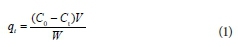
where q_t is the adsorptive capacity at time t, mg/g; C₀ is the initial concentration of ammonium in the solution, mg/L; C_t is the concentration of ammonium in the solution at time t, mg/L; V is the volume of the solution, L; and W is the mass of the adsorbent, g.

Adsorption isotherms for ammonium were carried out in thermostatic shakers for 24 h at desired temperatures (293, 303, 313 K). Adsorbents (0.5 g) were mixed with ammonium solutions (25 mL) at different initial concentrations ranging from 5 to 1 000 mg/L (5, 10, 25, 50, 100, 200, 500, 800, 1 000 mg/L) at pH 8. The order of exchange selectivity was evaluated by examining the concentrations of cations.

Adsorption kinetics for ammonium were evaluated at pH 8 and at an ambient temperature of 293 K. Adsorbents (0.5 g) were added to ammonium solutions (25 mL) with an initial concentration of 1 000 mg/L. Samples withdrawn at different time intervals of 0.25, 0.5, 1, 2, 3, 4, 8 and 12 h were analysed for ammonium concentration.

The regeneration study was performed by evaluating the effect of regeneration cycles on the ammonium adsorptive capacity at pH 8 and at an ambient temperature of 293 K. Adsorbents (0.5 g) were added in 25 mL of 1 000 mg/L ammonium solutions. The adsorbents were collected after adsorption and regenerated by 250 mL of 2 mol/L NaCl solution; the concentration of NaCl was consistent with the concentration used in the absorbent preparation. Then, the zeolites were washed by deionized water and centrifuged several times. The regenerated zeolite was reused for adsorption of ammonium from aqueous solution.

Analysis methods

Ammonium concentrations in liquid samples were analysed by spectrophotometry with a spectrophotometer (V-1100D, Mapada Co., Shanghai, China). The concentrations of Na⁺, K⁺, Ca²⁺ and Mg²⁺ in solution were measured by atomic absorption spectroscopy (AAS-6300C, Shimadzu, Japan). Elemental compositions of M-Zeo were determined using X-ray fluorescence (XRF) (XRF-1800, Shimadzu, Japan). Mineral phases were identified by X-ray diffraction (XRD) using a D/max-RB powder diffraction meter (Rigaku, Japan), with a Cu-target operated at 40 kV, 100 mA. The XRD patterns were taken in the range of 4-70° at a scan rate of 4°/min, which were analysed using the software (Search-Match) by comparing the experimental data with those included in the Joint Committee of Powder Diffraction Standards (JCPDSs) database.

 

RESULTS AND DISCUSSION

Characterization

XRD patterns of N-Zeo and M-Zeo are illustrated in Fig. 1. Diffraction patterns at 2θ = 9.88, 11.22, 17.34, 22.74, 26.12, 29.06, and 32° are identified as clinoptilolite when compared with the standard database. The characteristic peaks of quartz can be found at 26.7 and 50.1°. The intensity of quartz became weaker after modification. The XRD spectra of M-Zeo showed no significant differences from N-Zeo, indicating that the main mineral phases of zeolite were not changed after modification.

 

 

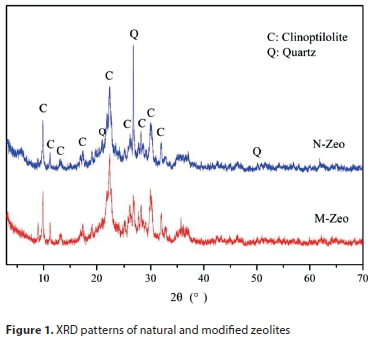
XRF was applied to analyse the elemental compositions of N-Zeo and M-Zeo, presented as percentage of element in the highest oxidation state (Table 1). It can be clearly seen that the contents of the exchangeable cations such as K⁺, Ca²⁺, and Mg²⁺ in the M-Zeo were decreased, while the amount of Na⁺ was increased significantly. The result suggested that Ca²⁺, K⁺, and Mg²⁺ were replaced by Na⁺, which can be used to remove NH₄⁺ in ion-exchange applications.

Effect of pH

Figure 2a shows the adsorption of ammonium onto N-Zeo and M-Zeo as a function of initial pH. In acidic condition, increasing pH favoured both N-Zeo and M-Zeo adsorption of ammonium. In basic conditions (pH 8 to 10), reduced adsorption capacity with increasing pH is seen in Fig. 2a, leading to the highest adsorption capacities of 11.39 and 17.77 mg/g on N-Zeo and M-Zeo, respectively, at pH 8. This clearly implies that ammonium adsorption onto both N-Zeo and M-Zeo was pH dependent. The dominant mechanism of ammonium adsorption onto N-Zeo and M-Zeo was assumed to be ion-exchange between cations (Na⁺, K⁺, Ca²⁺, Mg²⁺, et al.) on the adsorbent surface and ammonium in the solution. As shown in Fig. 2b, ammonium existed in the form of NH₄⁺ in aqueous solution at pH 2-8, and as NH₃ at pH 10-13. The species of ammonium were converted from NH₄⁺ to NH₃ when pH was between 8 and 10. At pH < 8, ammonium adsorption increased with increasing pH, principally being attributed to the decline in competing hydrogen ions, and with cation exchange being the dominant mechanism (Liu et al., 2013). At pH > 8, ammonium removal decreased with increasing pH, likely owing to the conversion of NH₄⁺ into NH₃ in alkaline solution. Thus, molecule adsorption was the main mechanism for ammonium removal, which resulted in the reduction of ion-exchange potential. This observation correlated with findings reported in the literature (He et al., 2016; Lin et al., 2013). Therefore, the optimum pH of M-Zeo for adsorption of ammonium is that of a neutral solution.

 

 

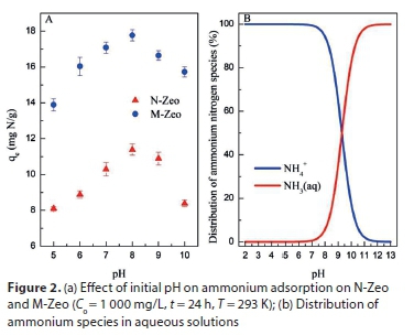
Ion-exchange adsorption

The ion exchange process between the zeolite frame and aqueous ammonium solution can be expressed by Eq. 2 (Lin et al., 2013):

where M represents the loosely held cations in zeolite and n is the number of electric charges. Assuming M in zeolite are Na⁺, K⁺, Ca²⁺ and Mg²⁺, the ion exchange capacity (IEC) can be calculated as the sum of exchange cations as follows:

As shown in Fig. 3, the adsorption capacity of ammonium onto M-Zeo increased significantly at different initial ammonium ion concentrations, while the equivalent concentrations of Mg²⁺, K⁺, Na⁺ and Ca²⁺ released into the solution increased significantly. The IEC for the sum of the four cations was a little lower than the ammonium adsorption capacity at equilibrium, indicating that ion exchange is predominant in the adsorption of ammonium by zeolite. The extra amount of ammonium adsorption on M-Zeo is ascribed to electrostatic attraction between negative charges on the adsorbent surface and NH₄⁺ (Alshameri, Ibrahim, et al., 2014).

 

 

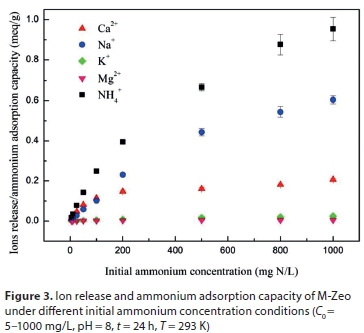
When the initial ammonium concentration rose to 25 mg/L, K⁺ started to be released from zeolite. Mg²⁺ appeared in the aqueous solution after the initial ammonium concentration rose to 50 mg/L. Na⁺ was the dominant cation exchanged with ammonia under an initial ammonia concentration of less than 100 mg/L, while Ca²⁺ was the dominant cation exchanged with ammonia under an initial ammonia concentration higher than 100 mg/L. Thus, the effect of the metal ions on ammonium adsorption to zeolite suggests an order of preference of Na⁺ > Ca²⁺ > K⁺ > Mg²⁺. A similar result was reported by other researchers (Lin et al., 2013). A slightl difference in the order was determined as Na⁺> K⁺> Ca²⁺ > Mg²⁺ by other researchers (Lei et al., 2008; Watanabe et al., 2007).

Adsorption isotherms

The adsorption isotherms of ammonium on zeolite were fitted by two typical models, Langmuir and Freundlich, as Eqs 4 and 5 (Liu et al., 2013; Langmuir, 1918):

where C_e is the equilibrium concentration (mg/L) in the solution; q_e is the adsorption capacity on adsorbent (mg/g); q_m refers to the maximum adsorption capacity at monolayer coverage (mg/g). The values of k (L/mg) and K_f (mg/g) are the Langmuir and Freundlich adsorption constants, respectively. 1/n is a constant relating to adsorption intensity or surface heterogeneity.

 

 

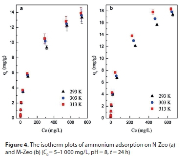
The relative parameters (q_m, k, K_f and 1/n) were calculated from the slope and intercept of the linear plots based on the Langmuir and Freundlich adsorption isotherms. As the correlation coefficient of the Freundlich model (R² > 0.9905) was higher than that of the Langmuir model (R² < 0.9815), the Freundlich model was suggested to better fit ammonium sorption onto both N-Zeo and M-Zeo. This indicated that adsorption occurred on a structurally heterogeneous adsorbent (Pan et al., 2017). The maximum adsorption capacity on a monomolecular layer of M-Zeo was estimated to be 17.83 mg/g at 293 K, which is higher than that found by other researchers. For example, Mazloomi and Jalali (2016) found the maximum adsorption of ammonium by Iranian zeolite to be 10.08 mg/g. Saltalı et al. (2007) reported that the adsorption capacity of ammonium by natural Turkish zeolite was 9.64 mg/g at 294 K (Saltali et al., 2007). It has also been reported that the maximum adsorption of ammonium using a salt-activated Chinese (Hulaodu) zeolite was 9.52 mg/g (Alshameri et al., 2014). Meanwhile the ammonium exchange capacity for natural and modified Yemeni zeolites were 11.18 mg/g and 8.29 mg/g, respectively (Alshameri et al., 2014). The constant of 1/n for the Freundlich model is related to the adsorption intensity, which varies with the heterogeneity of materials. The values of 1/n were lower than 0.52 in this study, which suggests that the adsorption of ammonium on N-Zeo and M-Zeo was highly favourable (Table 2).

The Dubinin-Redushckevich (D-R) isotherm was also employed to reveal the type of adsorption (physical adsorption or chemical adsorption) (Mazloomi and Jalali, 2016). The D-R equation has the linear form:

where q_m is the D-R adsorption capacity (mol/g); β is the constant of the adsorption energy (mol²/J²), related to the average energy of adsorption per mole of the sorbate as it is transferred to the surface of the solid from infinite distance in the solution; ε is Polanyi potential, which is described as:

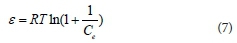
where T is the absolute temperature (K) and R is the gas constant (8.314 J/mol·K).

Moreover, the mean energy of adsorption E (kJ/mol) can be calculated from the D-R parameter β using the following formula:

As seen in Table 2, the correlation coefficients of the D-R model for ammonium sorption on N-Zeo and M-Zeo were higher than 0.977, suggesting the D-R model was acceptably applied to fit the experimental data in this study. The relative parameters (β and q_m) were calculated from the slope and intercept of Eq. 6. The value of mean energy of adsorption E is in the range of 1-8 kJ/mol and 8-16 kJ/mol for physical and chemical adsorption, respectively. In this study, the E values of ammonium adsorption on N-Zeo and M-Zeo were in the range of 8-16 kJ/mol, indicating that the adsorption process was essentially chemisorption (Table 2).

Thermodynamic parameters

The thermodynamic parameters can be calculated from the temperature-dependent adsorption isotherms based on Eqs 9-11:

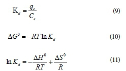
where K_d is the distribution coefficient, mL/g; ΔG⁰ is the change of Gibbs energy, kJ/mol. The values of enthalpy (ΔH⁰) and entropy (ΔS⁰) can be obtained by the slope and intercept of the plot of lnK_d versus 1/T (Fig. 5). The values of K_d, ΔG⁰, ΔH⁰ and ΔS⁰ are summarized in Table 3. Negative values of ΔG⁰ and positive values of ΔH⁰ were found, which reveals that the processes of ammonium adsorption on N-Zeo and M-Zeo were endothermic, feasible and spontaneous. The change of entropy (ΔS⁰) was 0.032 and 0.038 kJ/(mol·K) for the adsorption of ammonium on N-Zeo and M-Zeo, respectively. The positive values of ΔS⁰ suggested that the randomness increased during the removal of ammonium ions from aqueous solution onto N-Zeo and M-Zeo.

 

 

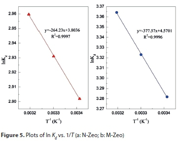
Adsorption kinetics

The adsorption kinetics of ammonium on M-Zeo and N-Zeo was simulated by four typical kinetic models. The kinetic equations, including pseudo first-order model, pseudo second-order model, Elovich model and intraparticle diffusion model, are described as follows (Huang et al., 2015; Malekian et al., 2011; Yang et al., 2015):

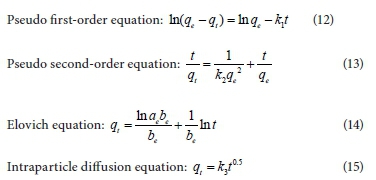
where q_t is the adsorbed amount at time t, mg/g; q_e is the adsorption amount at equilibrium, mg/g; k₁ is the rate constant of pseudo first-order adsorption, g/(mg·h); k₂ is the rate constant of pseudo second-order adsorption, g/(mg·h); the parameter a_e is the initial adsorption rate, mg/(g·h), and b_e is related to extent of surface coverage and activation energy for chemisorption, g/mg; k₃ is the intraparticle diffusion rate constant, mg/(g·h^−0.5).

Table 2 tabulates the relative parameters calculated from these four kinetic models. Constants k₁ and k₂ were respectively determined from the slope of the line obtained by plotting ln(q_e-q_t) versus t in the pseudo-first-order model and the intercept of the line by plotting t/q_t versus t in the pseudo-second-order model, while the initial adsorption rate a_e was determined from the intercept of the line obtained by plotting q_t versus ln t in the Elovich equation. The intraparticle diffusion rate constant k₃ was calculated from the slope of the line obtained by plotting q_t and t^0.5. The correlation coefficient for the pseudo-second-order model is the highest among the four kinetic models, revealing that the pseudo-second-order model best describes the adsorption kinetics of ammonium onto M-Zeo, and that chemisorption dominates in the adsorption process (Huang et al., 2017; Liao et al., 2012). This conclusion matched the fitting results from the D-R isotherm. Moreover, , the theoretically adsorbed amount at equilibrium (16.34 mg/g) obtained from the pseudo-second-order model was much closer to the adsorbed amount at equilibrium obtained from experiment (17.83 mg/g) than that obtained from the other models. Due to the high correlation coefficient (>0.99), the Elovich equation was also found to be suitable to describe the second-order kinetic, assuming that the actual solid surfaces are energetically heterogeneous (Mezenner and Bensmaili, 2009). The initial adsorption rate a_e was 49 166 mg/(g·h) for ammonium adsorption onto M-Zeo, which was much higher than 80.27 mg/(g·h) for ammonium adsorption onto N-Zeo. The intraparticle diffusion model is assumed to be the sole rate-controlling step if the regression of q_t versus t^0.5 is linear and the plots pass through the origin (Huang et al., 2010). The fitting results show that the regression was linear, but the plot did not pass through the origin. As seen in Fig. 6d, the ammonium adsorption onto N-Zeo and M-Zeo involved two steps and presented a multilinearity. Therefore, the adsorption processes of ammonium onto N-Zeo and M-Zeo can be divided into two steps. The first, fast step was mainly contributed by boundary layer diffusion or macro-pore diffusion. The second, gradual step was attributed to intraparticle diffusion or micro-pore diffusion (Pan et al., 2017; Widiastuti et al., 2011).

The apparent activation energy

The linear form of the Arrhenius equation can be expressed as the following formula:

where k is the rate constant of pseudo second-order adsorption; E_a is the apparent activation energy, J/mol; R is the gas constant, 8.314 J/mol·K; T is the absolute temperature (K).

Comparison of the outputs of adsorption kinetics models suggested that the adsorption process of ammonium onto N-Zeo and M-Zeo was in accordance with the pseudo-second order model. Thus, the apparent activation energy can be determined by the slope of the line plotting ln k (k₂ in Table 4) versus 1/T according to the Arrhenius equation. Chen (2016) stated that the reaction rate would be fast if E_a is less than 40 kJ/mol at room temperature, and rather slow if E_a is greater than 120 kJ/mol (Chen et al., 2016). Moreover, adsorption would be a diffusion-controlled process if the E_a is less than 25-30 kJ/mol (Lazaridis and Asouhidou, 2003; Mezenner and Bensmaili, 2009). In the present study, E_a was 13.37 kJ/mol for ammonium adsorption onto N-Zeo and ٩.٨٤ kJ/mol for ammonium adsorption onto M-Zeo, which was less than 25 kJ/mol. Thus, the adsorption of ammonium on M-Zeo was a fast and diffusion-controlled process and its reaction rate was much higher than the adsorption of ammonium on N-Zeo.

 

 

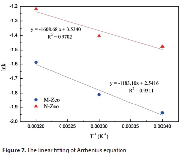
Regeneration and treatment of real wastewater

Fig. 8 shows the regeneration of M-Zeo after adsorbing ammonium. After being regenerated after the first cycle, the adsorption capacity of ammonium onto M-Zeo was slightly decreased from 17.36 mg/g to 16.77 mg/g. After 5 cycles in regeneration, the adsorption capacity had dropped to 15.73 mg/g and the regeneration ratio was up to 90.61%. A similar result was reported by Ji et al. (2007). Treatment of real wastewater by adsorbents could evaluate if the adsorbents can be used for environmental purification (Kostic et al., 2017; Kostic et al., 2018). In this study, sewage, which was collected from a domestic wastewater pipe at Xiamen University of Technology campus, with an initial ammonium concentration of 14.92 mg/L was employed to estimate the possibility of M-Zeo being used for real wastewater treatment. Under the condition of a pH value of 8.5 for the campus sewage, the final concentration of ammonium was 0.13 mg/L, indicating a removal efficiency for ammonium of 99.13%. Given the high removal efficiency and regeneration ratio of M-Zeo, it can be considered as a promising adsorbent in the preconcentration and removal of ammonium from aqueous solutions in environmental clean-ups.

 

 

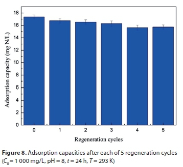
CONCLUSIONS

The synthetic M-Zeo was successfully prepared from N-Zeo by dispersing into NaCl solution and drying at 105°C. The adsorption isotherms and kinetics of ammonium by M-Zeo could be satisfactorily simulated by the Freundlich model and the pseudo-second-order model, respectively. Thermodynamic parameters indicated that the adsorption process of ammonium onto M-Zeo was endothermic and spontaneous. The fitting results of the D-R isotherm determined that ammonium removal by M-Zeo was chemisorption. According to the intraparticle diffusion model, ammonium adsorption onto M-Zeo involved two adsorption steps: (i) boundary layer diffusion or macro-pore diffusion, and (ii) intraparticle diffusion or micro-pore diffusion. The E_a in the Arrhenius equation suggested that the adsorption of ammonium on M-Zeo was a fast and diffusion-controlled process. The findings of this study suggest that the low cost, high adsorption capacity and good regeneration performance of M-Zeo indicate that it is a promising adsorbent to be widely utilized for ammonium removal from aqueous solution.

 

ACKOWLEDGEMENTS

The authors would like to express their gratitude for the financial support provided by the Natural Science Foundation of Fujian Province, China (2016J05140), the Open Research Fund Program from Key Laboratory of Environmental Biotechnology (XMUT), Fujian Province University (EBL2018004), the Scientific Research Project of Xiamen Overseas Talents (201631402), Scientific Climbing Program of Xiamen University of Technology (XPDKQ18031) and the Science and Technology Project of Longyan City (2017LY63).

 

REFERENCES

ALSHAMERI A, IBRAHIM A, ASSABRI AM, LEI X, WANG H and YAN C (2014) The investigation into the ammonium removal performance of Yemeni natural zeolite: Modification, ion exchange mechanism, and thermodynamics. Powder Technol. 258 20-31. https://doi.org/10.1016/j.powtec.2014.02.063        [ Links ]

ALSHAMERI A, YAN C, AL-ANI Y, DAWOOD AS, IBRAHIM A, ZHOU C and WANG H (2014) An investigation into the adsorption removal of ammonium by salt activated Chinese (Hulaodu) natural zeolite: Kinetics, isotherms, and thermodynamics. J. Taiwan Inst. Chem. Eng. 45 554-564. https://doi.org/10.1016/j.jtice.2013.05.00        [ Links ]

CHEN F, ZHOU C, LI G and PENG F (2016) Thermodynamics and kinetics of glyphosate adsorption on resin D301. Arab. J. Chem. 9 S1665-S1669. https://doi.org/10.1016/j.arabjc.2012.04.014        [ Links ]

DARAMOLA M, ARANSIOLA E and OJUMU T (2012) Potential applications of zeolite membranes in reaction coupling separation processes. Materials 5 2101-2136. https://doi.org/10.3390/ma5112101        [ Links ]

HE Y, LIN H, DONG Y, LIU Q and WANG L (2016) Simultaneous removal of ammonium and phosphate by alkaline-activated and lanthanum-impregnated zeolite. Chemosphere 164 387-395. https://doi.org/10.1016/j.chemosphere.2016.08.110        [ Links ]

HUANG H, XIAO X, YAN B and YANG L (2010) Ammonium removal from aqueous solutions by using natural Chinese (Chende) zeolite as adsorbent. J. Hazardous Mater. 175 247-252. https://doi.org/10.1016/j.jhazmat.2009.09.156        [ Links ]

HUANG H, YANG L, XUE Q, LIU J, HOU L and DING L (2015) Removal of ammonium from swine wastewater by zeolite combined with chlorination for regeneration. J. Environ. Manage. 160 333-341. https://doi.org/10.1016/j.jenvman.2015.06.039        [ Links ]

HUANG X, CHEN T, ZOU X, ZHU M, CHEN D and PAN M (2017) The Adsorption of Cd(II) on Manganese oxide investigated by batch and modeling techniques. Int. J. Environ. Res. Public Health 14 1145-1155. https://doi.org/10.3390/ijerph14101145        [ Links ]

HUSSAIN S, AZIZ HA, ISA MH, ADLAN MN and ASAARI FA (2007) Physico-chemical method for ammonia removal from synthetic wastewater using limestone and GAC in batch and column studies. Bioresour. Technol. 98 874-880. https://doi.org/10.1016/j.biortech.2006.03.003        [ Links ]

JI ZY, YUAN JS and LI XG (2007) Removal of ammonium from wastewater using calcium form clinoptilolite. J. Hazardous Mater. 141 483-488. https://doi.org/10.1016/j.jhazmat.2006.07.010        [ Links ]

KARAPINAR N (2009) Application of natural zeolite for phosphorus and ammonium removal from aqueous solutions. J. Hazardous Mater. 170 1186-1191. https://doi.org/10.1016/j.jhazmat.2009.05.094        [ Links ]

KOLAKOVIC S, STEFANOVIC D, LEMIC J, MILICEVIC D, TOMOVIC S, TRAJKOVIC S and MILENKOVIC S (2014) Forming a filter media from zeolite modified with SDBAC for wastewater treatment process. Chem. Ind. Chem. Eng. Q. 20 361-369. https://doi.org/10.2298/ciceq121218018k        [ Links ]

KOSTIC M, DORDEVIC M, MITROVIC J, VELINOV N, BOJIC D, ANTONIJEVIC M and BOJIC A (2017) Removal of cationic pollutants from water by xanthated corn cob: optimization, kinetics, thermodynamics, and prediction of purification process. Environ. Sci. Pollut. Res. Int. 24 17790-17804. https://doi.org/10.1007/s11356-017-9419-1        [ Links ]

KOSTIC M, RADOVIC M, VELINOV N, NAJDANOVIC S, BOJIC D, HURT A and BOJIC A (2018) Synthesis of mesoporous triple-metal nanosorbent from layered double hydroxide as an efficient new sorbent for removal of dye from water and wastewater. Ecotoxicol. Environ. Saf. 159 332-341. https://doi.org/10.1016/j.ecoenv.2018.05.015        [ Links ]

LANGMUIR I (1918) The adsorption of gases on plane surfaces of glass, mica and platinum. J. Am. Chem. Soc. 40 1316-1403. https://doi.org/10.1021/ja02242a004        [ Links ]

LAZARIDIS NK and ASOUHIDOU DD (2003) Kinetics of sorptive removal of chromium(VI) from aqueous solutions by calcined Mg-Al-CO₃ hydrotalcite. Water Res. 37 2875-2882. https://doi.org/10.1016/s0043-1354(03)00119-2        [ Links ]

LEI L, LI X and ZHANG X (2008) Ammonium removal from aqueous solutions using microwave-treated natural Chinese zeolite. Sep. Purif. Technol. 58 359-366. https://doi.org/10.1016/j.seppur.2007.05.008        [ Links ]

LI M, ZHU X, ZHU F, REN G, CAO G and SONG L (2011) Application of modified zeolite for ammonium removal from drinking water. Desalination 271 295-300. https://doi.org/10.1016/j.desal.2010.12.047        [ Links ]

LIAO P, YUAN S, ZHANG W, TONG M and WANG K (2012) Mechanistic aspects of nitrogen-heterocyclic compound adsorption on bamboo charcoal. J. Colloid Interf. Sci. 382 74-81. https://doi.org/10.1016/j.jcis.2012.05.052        [ Links ]

LIN L, LEI Z, WANG L, LIU X, ZHANG Y, WAN C, LEE D-J and TAY JH (2013) Adsorption mechanisms of high-levels of ammonium onto natural and NaCl-modified zeolites. Sep. Purif. Technol. 103 15-20. https://doi.org/10.1016/j.seppur.2012.10.005        [ Links ]

LIU H, PENG S, SHU L, CHEN T, BAO T and FROST RL (2013) Effect of Fe₃O₄ addition on removal of ammonium by zeolite NaA. J. Colloid Interf. Sci. 390 204-210. https://doi.org/10.1016/j.jcis.2012.09.010        [ Links ]

LIU Z, CHEN L, ZHANG Z, LI Y, DONG Y and SUN Y (2013) Synthesis of multi-walled carbon nanotube-hydroxyapatite composites and its application in the sorption of Co(II) from aqueous solutions. J. Mol. Liq. 179 46-53. https://doi.org/10.1016/j.molliq.2012.12.011        [ Links ]

MALEKIAN R, ABEDI-KOUPAI J, ESLAMIAN SS, MOUSAVI SF, ABBASPOUR KC and AFYUNI M (2011) Ion-exchange process for ammonium removal and release using natural Iranian zeolite. Appl. Clay. Sci. 51 323-329. https://doi.org/10.1016/j.clay.2010.12.020        [ Links ]

MAZLOOMI F and JALALI M (2016) Ammonium removal from aqueous solutions by natural Iranian zeolite in the presence of organic acids, cations and anions. J. Environ. Chem. Eng. 4 1664-1673. https://doi.org/10.1016/j.jece.2015.11.031        [ Links ]

MEZENNER NY and BENSMAILI A (2009) Kinetics and thermodynamic study of phosphate adsorption on iron hydroxide-eggshell waste. Chem. Eng. J. 147 87-96. https://doi.org/10.1016/j.cej.2008.06.024        [ Links ]

ONYANGO M, KITTINYA J, HADEBE N, OJIJO V and OCHIENG A (2011) Sorption of melanoidin onto surfactant modified zeolite. Chem. Ind. Chem. Eng. Q. 17 385-395. https://doi.org/10.2298/ciceq110125025o        [ Links ]

PAN M, HU Z, LIU R and ZHAN X (2015) Effects of loading rate and aeration on nitrogen removal and N₂O emissions in intermittently aerated sequencing batch reactors treating slaughterhouse wastewater at 11°C. Bioprocess Biosyst. Eng. 38 681v689. https://doi.org/10.1007/s00449-014-1307-1        [ Links ]

PAN M, HUANG X, WU G, HU Y, YANG Y and ZHAN X (2017) performance of denitrifying phosphate removal via nitrite from slaughterhouse wastewater treatment at low temperature. Water 9 818. https://doi.org/10.3390/w9110818        [ Links ]

PAN M, LIN X, XIE J and HUANG X (2017) Kinetic, equilibrium and thermodynamic studies for phosphate adsorption on aluminum hydroxide modified palygorskite nano-composites. RSC Adv. 7 4492-4500. https://doi.org/10.1039/c6ra26802a        [ Links ]

SALTALI K, SARI A and AYDIN M (2007) Removal of ammonium ion from aqueous solution by natural Turkish (Yildizeli) zeolite for environmental quality. J. Hazardous Mater. 141 258-263. https://doi.org/10.1016/j.jhazmat.2006.06.124        [ Links ]

SARIOGLU M (2005) Removal of ammonium from municipal wastewater using natural Turkish (Dogantepe) zeolite. Sep. Purif. Technol. 41 1-11. https://doi.org/10.1016/j.seppur.2004.03.008        [ Links ]

WANG Y, LIN F and PANG W (2008) Ion exchange of ammonium in natural and synthesized zeolites. J. Hazardous Mater. 160 371-375. https://doi.org/10.1016/j.jhazmat.2008.03.006        [ Links ]

WATANABE Y, YAMADA H, KOKUSEN H, TANAKA J, MORIYOSHI Y and KOMATSU Y (2007) Ion exchange behavior of natural zeolites in distilled water, hydrochloric acid, and ammonium chloride solution. Sep. Sci. Technol. 38 1519-1532. https://doi.org/10.1081/ss-120019090        [ Links ]

WIDIASTUTI N, WU H, ANG HM and ZHANG D (2011) Removal of ammonium from greywater using natural zeolite. Desalination 277 15-23. https://doi.org/10.1016/j.desal.2011.03.030        [ Links ]

YANG S, DING C, CHENG W, JIN Z and SUN Y (2015) Effect of microbes on Ni(II) diffusion onto sepiolite. J. Mol. Liq. 204 170-175. https://doi.org/10.1016/j.molliq.2015.01.035        [ Links ]

ZHAO Y, ZHANG B, ZHANG X, WANG J, LIU J and CHEN R (2010) Preparation of highly ordered cubic NaA zeolite from halloysite mineral for adsorption of ammonium ions. J. Hazardous Mater. 178 658-664. https://doi.org/10.1016/j.jhazmat.2010.01.136        [ Links ]

 

 

Received 16 September 2018
Accepted in revised form 27 September 2019

 

 

* Corresponding author, email: huangxman@vip.sina.com

^rND^sALSHAMERI^nA^rND^sIBRAHIM^nA^rND^sASSABRI^nAM^rND^sLEI^nX^rND^sWANG^nH^rND^sYAN^nC^rND^sALSHAMERI^nA^rND^sYAN^nC^rND^sAL-ANI^nY^rND^sDAWOOD^nAS^rND^sIBRAHIM^nA^rND^sZHOU^nC^rND^sWANG^nH^rND^sCHEN^nF^rND^sZHOU^nC^rND^sLI^nG^rND^sPENG^nF^rND^sDARAMOLA^nM^rND^sARANSIOLA^nE^rND^sOJUMU^nT^rND^sHE^nY^rND^sLIN^nH^rND^sDONG^nY^rND^sLIU^nQ^rND^sWANG^nL^rND^sHUANG^nH^rND^sXIAO^nX^rND^sYAN^nB^rND^sYANG^nL^rND^sHUANG^nH^rND^sYANG^nL^rND^sXUE^nQ^rND^sLIU^nJ^rND^sHOU^nL^rND^sDING^nL^rND^sHUANG^nX^rND^sCHEN^nT^rND^sZOU^nX^rND^sZHU^nM^rND^sCHEN^nD^rND^sPAN^nM^rND^sHUSSAIN^nS^rND^sAZIZ^nHA^rND^sISA^nMH^rND^sADLAN^nMN^rND^sASAARI^nFA^rND^sJI^nZY^rND^sYUAN^nJS^rND^sLI^nXG^rND^sKARAPINAR^nN^rND^sKOLAKOVIC^nS^rND^sSTEFANOVIC^nD^rND^sLEMIC^nJ^rND^sMILICEVIC^nD^rND^sTOMOVIC^nS^rND^sTRAJKOVIC^nS^rND^sMILENKOVIC^nS^rND^sKOSTIC^nM^rND^sDORDEVIC^nM^rND^sMITROVIC^nJ^rND^sVELINOV^nN^rND^sBOJIC^nD^rND^sANTONIJEVIC^nM^rND^sBOJIC^nA^rND^sKOSTIC^nM^rND^sRADOVIC^nM^rND^sVELINOV^nN^rND^sNAJDANOVIC^nS^rND^sBOJIC^nD^rND^sHURT^nA^rND^sBOJIC^nA^rND^sLANGMUIR^nI^rND^sLAZARIDIS^nNK^rND^sASOUHIDOU^nDD^rND^sLEI^nL^rND^sLI^nX^rND^sZHANG^nX^rND^sLI^nM^rND^sZHU^nX^rND^sZHU^nF^rND^sREN^nG^rND^sCAO^nG^rND^sSONG^nL^rND^sLIAO^nP^rND^sYUAN^nS^rND^sZHANG^nW^rND^sTONG^nM^rND^sWANG^nK^rND^sLIN^nL^rND^sLEI^nZ^rND^sWANG^nL^rND^sLIU^nX^rND^sZHANG^nY^rND^sWAN^nC^rND^sLEE^nD-J^rND^sTAY^nJH^rND^sLIU^nH^rND^sPENG^nS^rND^sSHU^nL^rND^sCHEN^nT^rND^sBAO^nT^rND^sFROST^nRL^rND^sLIU^nZ^rND^sCHEN^nL^rND^sZHANG^nZ^rND^sLI^nY^rND^sDONG^nY^rND^sSUN^nY^rND^sMALEKIAN^nR^rND^sABEDI-KOUPAI^nJ^rND^sESLAMIAN^nSS^rND^sMOUSAVI^nSF^rND^sABBASPOUR^nKC^rND^sAFYUNI^nM^rND^sMAZLOOMI^nF^rND^sJALALI^nM^rND^sMEZENNER^nNY^rND^sBENSMAILI^nA^rND^sONYANGO^nM^rND^sKITTINYA^nJ^rND^sHADEBE^nN^rND^sOJIJO^nV^rND^sOCHIENG^nA^rND^sPAN^nM^rND^sHU^nZ^rND^sLIU^nR^rND^sZHAN^nX^rND^sPAN^nM^rND^sHUANG^nX^rND^sWU^nG^rND^sHU^nY^rND^sYANG^nY^rND^sZHAN^nX^rND^sPAN^nM^rND^sLIN^nX^rND^sXIE^nJ^rND^sHUANG^nX^rND^sSALTALI^nK^rND^sSARI^nA^rND^sAYDIN^nM^rND^sSARIOGLU^nM^rND^sWANG^nY^rND^sLIN^nF^rND^sPANG^nW^rND^sWATANABE^nY^rND^sYAMADA^nH^rND^sKOKUSEN^nH^rND^sTANAKA^nJ^rND^sMORIYOSHI^nY^rND^sKOMATSU^nY^rND^sWIDIASTUTI^nN^rND^sWU^nH^rND^sANG^nHM^rND^sZHANG^nD^rND^sYANG^nS^rND^sDING^nC^rND^sCHENG^nW^rND^sJIN^nZ^rND^sSUN^nY^rND^sZHAO^nY^rND^sZHANG^nB^rND^sZHANG^nX^rND^sWANG^nJ^rND^sLIU^nJ^rND^sCHEN^nR^rND^1A01^nHassan^sHeidari^rND^1A01^nSaman^sMoradi^rND^1A01^nHassan^sHeidari^rND^1A01^nSaman^sMoradi^rND^1A01^nHassan^sHeidari^rND^1A01^nSaman^sMoradi

RESEARCH PAPERS

 

Comparison of refined and non-refined wastewater effect on wheat seed germination and growth under drought

 

 

Hassan Heidari^*; Saman Moradi

Department of Agronomy and Plant Breeding, Faculty of Agricultural Science and Engineering, Razi University, Kermanshah, Iran

 

 

---

ABSTRACT

Wastewater has attracted special attention as a possible source of irrigation. The present study aimed to compare the effect of refined and non-refined wastewater on wheat seed germination and growth under induced drought conditions in laboratory and pot experiments. The laboratory experiment included the iso-osmotic potentials of −0.275, −0.4, and −0.47 MPa of polyethylene glycol (PEG, as a drought factor) and wastewater. In addition, the pot experiment included a wastewater factor (i.e., tap water, 100% refined wastewater, 50% refined wastewater + 50% non-refined wastewater, and 100% non-refined wastewater) and a drought factor (i.e., an irrigation interval of two and three days as normal and drought conditions, respectively). The results demonstrated that the drought related to PEG did not reduce seed germination while wastewater decreased seed germination. Further, an osmotic potential of −0.47 MPa resulted in the highest and lowest radicle length in both wastewater and PEG, respectively. The results also revealed that caulicle length and seed vigour were decreased by PEG as the osmotic potential increased while no significant difference was observed between wastewater treatments and distilled water (control). Based on the results, an irrigation interval of 3 days with 100% non-refined wastewater produced the highest chlorophyll content and 100% refined and 100% non-refined wastewater produced a larger leaf area compared to the control. Furthermore, drought with wastewater application increased specific leaf weight whereas it reduced the total biomass compared to control (i.e., tap water with an irrigation interval of 2 days), except for 100% non-refined wastewater. Therefore, wastewater application compensates for the adverse effect of drought due to nutrient addition.

Keywords: chlorophyll, drought, refined wastewater, seed vigour

---

 

 

INTRODUCTION

Drought is considered to be one of the most important factors which limits crop production across the globe. Agricultural production should be increased to meet global population demands (Tilman et al., 2011). Irrigation is regarded as one of the methods which effectively increases crop production while water use efficiency typically remains stable under different water amounts (Curt et al., 1995). According to Mustafa Tahir et al. (2014), shortening the irrigation interval at the critical periods of growth can lead to an increase in plant height and forage yield for oats.

Chlorophyll concentration is a key factor in photosynthesis rate (Ghosh et al., 2004), which increases under drought since leaf area reduces and the leaf becomes thicker, leading to an increase in chlorophyll concentration (Barraclough and Kate, 2001).

Wastewater (e.g., domestic and industrial types) can be used for crop irrigation. In addition, it has been found to increase plant height and biomass in wheat (Pandey and Singh, 2015). According to Ashraf and Ali (2007), seed germination is one of the sensitive stages in plant growth and, as an index of plant sensitivity to contamination, has attracted the attention of different studies. Wastewater contains salts and heavy metals. Li et al. (2005) reported that an increase in heavy metal concentration caused a decline in seed germination percentage. The highest wheat seed germination was recorded at 25% effluent concentration when compared to a variety of other concentrations (e.g., 0%, 25%, 50%, 75%, and 100%) of effluents from a textile and sugar factory (Nandal et al., 2017). Seedling root and shoot growth decreased relative to a control when applying effluents from a pharmaceutical and battery industry at various irrigation intervals (Raju et al., 2015).

However, various studies have reported different adverse effects of salinity and drought. Both salinity and drought reduce coleoptile and root length, as well as the fresh and dry weight of the root and coleoptiles in wheat (Jovovic et al., 2018). The drought and salinity in these studies resulted from polyethylene glycol and NaCl, respectively, and had no significant effect on seed germination percentage, germination rate, or seedling shoot and root weight in wheat, compared to the control (Mohammadi and Dargahi, 2015). Farmers may use wastewater for irrigation, in refined or non-refined form, from different sources including a domestic source. Further, physical and chemical processes may be utilized for treating the wastewater (Mlakar et al., 2017). The application of non-refined wastewater for irrigation can inhibit plant growth through cell division, due to sticky and lagging chromosomes (Sik et al., 2009), and irrigating plants with non-refined wastewater may cause disease if directly applied by a person. Conversely, several other studies have indicated that non-refined wastewater can promote plant growth (Moradi et al., 2016; Khaleel et al., 2013).

It is not clear whether refined wastewater can have the same promoting effect as non-refined wastewater. Furthermore, wastewater refinement is a costly process and its efficiency needs evaluation. Therefore, the current study sought to compare physical, chemical, and biological traits of refined and non-refined wastewater and their effects on seed germination and early plant growth in wheat under drought.

 

MATERIALS AND METHODS

Laboratory experiment

A laboratory experiment was conducted at Physiology Laboratory, the College of Agricultural Science and Engineering, Razi University, during 2014. Based on the aim of the study, the treatments encompassed the iso-osmotic potentials of −0.275, −0.4, and −0.47 MPa (equal to 100% refined wastewater, 50% refined wastewater + 50% non-refined wastewater, and 100% non-refined wastewater, respectively), of polyethylene glycol (PEG, as a drought factor) and refined or non-refined wastewater. Table 1 demonstrates some of the parameters of refined and non-refined wastewater. PEG solutions were prepared according to Michel and Kaufmann's formula (1973):

 

 

 

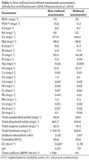
where: Y_s, C, and T demonstrate the osmotic potential, the concentration of PEG in g∙kg⁻¹ H₂O, and the temperature in degrees Celsius, respectively. The osmotic potentials of wastewater were measured using an osmometer and distilled water was utilized as a control. Therefore, the experiment comprised 7 treatments (i.e., one control and −0.275, −0.4, and −0.47 MPa of polyethylene glycol and wastewater). The study was conducted as a completely randomized design with 3 replications. Ghareso is a river in Kermanshah and the wastewaters from industrial and domestic sources are discharged into this river. Additionally, a wastewater treatment plant exists in Kermanshah to purify part of the effluents. In general, the purification process occurs in 3 steps: physical purification, which encompasses the construction of overflow, screens, the initial sedimentation ponds, the secondary sedimentation ponds, and the pump house of the sludge; chemical purification, which involves activated sludge and chlorination pools; and, finally, biological treatment, which involves biological reactors (Iran's Environmental Health, 2019). Wastewater samples were collected from Kermanshah wastewater treatment plant with an output of 60 000 m³∙day⁻¹ (Ghamarnia et al., 2014), which serves 400 000 persons.

To assess the effect of wastewater and drought on seed germination, the seeds of wheat (Triticum aestivum cv. Sirwan) were placed on filter paper in Petri dishes and then 6 mL of the prepared solution was added to each Petri dish. Next, these dishes were kept in a germinator for a week, after which several parameters were measured: seed germination percentage, caulicle length, radicle length, radicle to caulicle ratio, and seed vigour. Seed vigour was calculated by Heidari's (2013) equation.

Pot experiment

An outdoor pot experiment was conducted at the College of Agricultural Science and Engineering, Razi University, in 2014. The experiment was conducted as a factorial arrangement based on a randomized complete block design with 3 replicates. One factor was wastewater (i.e., tap water, 100% refined wastewater, 50% refined wastewater + 50% non-refined wastewater, and 100% non-refined wastewater). The other factor included irrigation intervals (2 and 3 days) which were determined by a pre-experiment. In the pre-experiment, the irrigation intervals of 2 and 3 days were determined as well-watered and drought treatments, respectively, based on soil factors and plant symptoms. At each irrigation event, the soil surface was gradually watered to ensure the soil was totally wet. Then, watering was stopped when the pot soil started to drain and the seeds of the wheat (Triticum aestivum cv. Sirwan) were sown in pots (7 cm in diameter and 7.5 cm in height) filled by field soil. The experiment lasted 21 days, after which related parameters were estimated: leaf chlorophyll content, plant height, leaf area, stem fresh and dry weight, leaf fresh and dry weight, leaf to stem ratio, total biomass, and specific leaf weight. Specific leaf weight was calculated by dividing leaf dry weight by leaf area. A SPAD (soil plant analytical development) device was used to determine the index of leaf chlorophyll (Bail et al., 2005). Finally, leaf and stem samples were dried in an oven at 70°C for 24 h in order to calculate their dry weight.

Data analysis

Data were analysed by SAS software and the means were compared by applying Duncan's multiple range test at a probability level of 5%.

 

RESULTS

Water quality

The effluent quality was improved by the wastewater treatment plant (Table 1). For example, heavy metals, as well as some essential nutrients for plant growth, such as nitrogen and phosphorus, were reduced by wastewater treatment. Fe increase could be attributed to FeCl₃ for coagulation. Mn increase could be due to the lack of subsurface oxygen. pH increase could be attributed to liming.

Laboratory experiment

Figure 1 illustrates the influence of polyethylene glycol (PEG) iso-osmotic potentials and wastewater on the seed germination traits of wheat. Drought related to PEG fails to reduce seed germination while wastewater decreases it (Fig. 1a). Further, germination reduction by wastewater is initiated by the lowest osmotic potential. The osmotic potential of −0.47 MPa for the wastewater and PEG resulted in the highest and lowest radicle length, respectively (Fig. 1b). An increase in osmotic potential leads to a decrease in the caulicle length with PEG, whereas no significant difference is observed between wastewater treatments and distilled water as control (Fig. 1c). With regard to the radicle to caulicle ratio, there is also no significant difference between wastewater treatments and distilled water (Fig. 1d). Furthermore, seed vigour decreases with PEG through increasing the osmotic potential, while wastewater treatments and distilled water demonstrate no significant difference in terms of seed vigour (Fig. 1e).

 

 

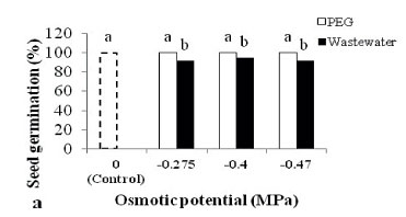
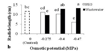
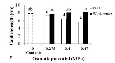
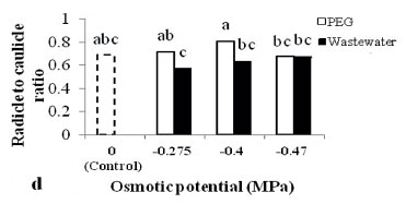
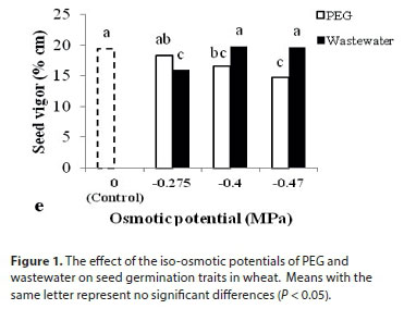
Pot experiment

The effect of irrigation interval and wastewater on early growth traits in wheat is displayed in Fig. 2. The irrigation interval of 3 days with 100% non-refined wastewater produces the highest chlorophyll content. More precisely, drought reduces leaf area while increasing leaf thickness (specific leaf weight), leading to an increase in chlorophyll concentration which is confirmed by the results of the current experiment (Fig. 2a). Under the irrigation interval of 2 days, leaf fresh weight increases for all wastewater treatments whereas under the irrigation interval of 3 days, only 100% non-refined wastewater results in an increase in leaf fresh weight (Fig. 2b). Drought reduces leaf dry weight (Fig. 2c). Additionally, 100% refined wastewater produces the highest stem dry weight. A remarkable reduction of some nutrients while improving some physiochemical properties of wastewater (e.g., electrical conductivity) in 100% refined wastewater results in increasing the stem dry weight (Fig. 2d). In addition, 100% refined wastewater with an irrigation interval of 2 days reveals higher plant height compared to the control, namely, tap water with an irrigation interval of 2 days. By increasing the irrigation interval, the height of the plant irrigated by 100% non-refined wastewater shows no reduction (Fig. 2e), which is likely due to the positive effect of wastewater on plant growth. Further, 100% refined and 100% non-refined wastewater produce a higher leaf area compared to the control (Fig. 2f). The lowest and highest leaf to stem ratio, among the treatments, is observed for 100% refined wastewater with an irrigation interval of 2 and 3 days, respectively (Fig. 2g). On the other hand, drought increases leaf to stem ratio under 100% refined wastewater. This suggests that stem elongation initiation is postponed by drought. Additionally, drought with wastewater application leads to an increase in specific leaf weight compared to the control (Fig. 2h), and finally, drought reduces total biomass compared to the control, except in the case of 100% wastewater (Fig. 2i).

 

DISCUSSION

Laboratory experiment

The reduction in seed germination by wastewater can be attributed to salinity and heavy metal stresses, which is confirmed by the data in Table 1. Further, higher electrical conductivity and some inhibiting elements, including Na, in the wastewater are the main reasons for such a reduction in seed germination. Apparently, salinity stress had a negative effect on germination while some nutrients promoted radicle and caulicle length after germination in the present study. However, these nutrients demonstrated their effect only at high concentration. The adverse effect of osmotic potential was compensated for by the positive effect of wastewater due to nutrients (Li et al., 2005). Raju et al. (2015) also reported a decline in wheat seed germination due to effluent from a pharmaceutical and battery industry, which is in line with the results of the current study. Furthermore, some other studies found that seed priming by sodium compounds such as sodium silicate (Hameed et al., 2013) and sodium nitroprusside (Ali et al., 2017) enhance seedling root and shoot growth in wheat due to a reduction in the oxidative stress of salinity. This corroborates the results of the present study. Contrary to the results of the current study, Sayar et al. (2010) concluded that drought stress resulting from polyethylene glycol (PEG) had a higher adverse effect on germination percentage in wheat compared to NaCl-related salinity. Additionally, PEG-induced drought stress had an even more negative effect on radicle to caulicle ratio compared to wastewater (Fig. 1d). Essential nutrients available in wastewater reduced the negative effects of drought. Saidi et al. (2010) reported that root weight increases in wheat seedlings under increasing drought. Seed treated with wastewater represented higher seed vigour under the osmotic potential of −0.4 and −0.47 MPa, compared to the seed treated with PEG (Fig. 1e). The results of another study indicated that NaCl had a more adverse effect on germination compared to drought (Al-taisan, 2010) while other studies have reported that drought had a more adverse effect on germination compared to NaCl (e.g., Okcu et al., 2005; Rahimi et al., 2006).

Pot experiment

Heidari et al. (2011) found an increase in the chlorophyll content of water-stressed plants while Abdalla and El-khoshiban (2007) reported that drought reduced the chlorophyll content. This contradiction can be attributed to stress severity. In other words, chlorophyll is destroyed under severe drought which leads to a decrease in its content. In this respect, the effect of wastewater should be considered as well. Wastewater contains essential nutrients, including nitrogen, for plant growth and chlorophyll formation, and chlorophyll content, as one of source strength components, is affected by wastewater (Ghosh et al., 2004). In addition, 100% non-refined wastewater contains more nutrients than tap water and refined wastewater (Table 1). Leaf fresh weight mainly relies on leaf moisture and its trend indicates that wastewater salts may be absorbed by plant tissues. Further, salts accumulate water, thus the leaf becomes succulent (Sen and Rajpurohit, 2012) and drought reduces leaf dry weight. In the present study, the comparison of leaf dry and fresh weight revealed that wastewater increased leaf moisture (Fig. 2). According to Alyemeny (1998), a reduction in leaf biomass helps the plant to tolerate water deficit, and plant height reduction as a result of drought is considered as an adaptation response of plants in order to reduce transpiration (Karam et al., 2003). Furthermore, drought decreases cell size and internode length (Ludlow et al., 1990). However, based on the results of the current study, drought did not reduce leaf area for the 100% non-refined wastewater treatment (Fig. 2). A larger amount of nutrients such as nitrogen and phosphorus in 100% non-refined wastewater plays a role in chlorophyll production and increasing leaf area, compared to refined wastewater. Additionally, drought diminishes cell elongation and division, and thus reduces leaf area. Other studies, including Karam et al. (2003), have reported leaf area reduction due to drought as well. In addition, the results of the present study confirm that drought reduces the leaf area and increases the leaf thickness, leading to an increase in specific leaf weight (Fig. 2). The results further indicate that wastewater can promote plant growth by increasing the leaf thickness in order to capture more radiant energy. Water deficit leads to various morpho-physiological changes in the plants. For example, leaf growth is inhibited first, before photosynthesis and respiration, when there is a reduction in water potential, and soil water deficit reduces xylem sap movement toward the leaves (Liptay et al., 1998).

 

CONCLUSIONS

In general, an osmotic potential of −0.47 MPa of wastewater, resulted in the lowest seed germination percentage. Further, wastewater at low water potential failed to reduce seed germination traits such as seed vigour, while using polyethylene glycol to create a low osmotic potential decreased these traits. It is likely that the positive physiochemical properties of wastewater, including nitrogen content, acted to promote plant growth. Furthermore, plants irrigated with 100% refined wastewater under the well-watered condition produced the highest total biomass, since 100% refined wastewater contained growth-promoting ingredients such as nitrogen and phosphorus. Based on the results, drought reduced different growth parameters such as leaf and stem dry weight whereas wastewater application compensated for the negative effect of drought. Finally, drought decreased total biomass compared to control, except in the case of the 100% wastewater treatments. Therefore, irrigation of wheat with wastewater is recommended after germination instead of at the germination stage, and irrigation with refined wastewater can promote plant growth.

 

REFERENCES

ABDALLA MM and EL-KHOSHIBAN NH (2007) The influence of water stress on growth, relative water content, photosynthetic pigments, some metabolic and hormonal contents of two Triticium aestivum cultivars. J. Appl. Sci. Res. 3 (12) 2062-2074.         [ Links ]

ALI Q, DAUD MK, HAIDER MZ, ALI S, RIZWAN M, ASLAM N, NOMAN A, IQBAL N, SHAHZAD F, DEEBA F, ALI I and ZHU SJ (2017) Seed priming by sodium nitroprusside improves salt tolerance in wheat (Triticum aestivum L.) by enhancing physiological and biochemical parameters. Plant Physiol. Biochem. 119 50-58. https://doi.org/10.1016/j.plaphy.2017.08.010        [ Links ]

AL-TAISAN WA (2010) Comparative effects of drought and salt stress on germination and seedling growth of Pennisetum divisum (Gmel.) Hener. Am. J. Appl. Sci. 7 640-646. https://doi.org/10.3844/ajassp.2010.640.646        [ Links ]

ALYEMENY MN (1998) The effect of drought on growth and dry matter allocation in seedling of Vigna ambacensis L. J. King Saud Univ. 10 41-51.         [ Links ]

ASHRAF R and ALI TA (2007) Effect of heavy metals on soil microbial community and mung beans seed germination. Pak. J. Bot. 39 629-636.         [ Links ]

BAIL ML, JEUFFROY MH, BOUCHARD C and BARBORTIN A (2005) Is it possible to forecast the grain quality and yield of different varieties of winter wheat from Minolta SPAD Meter measurement? Eur. J. Agron. 23 379. https://doi.org/10.1016/j.eja.2005.02.003        [ Links ]

BARRACLOUGH PB and KATE J (2001) Effect of water stress on chlorophyll meter reading in wheat. Plant Nutr. 92 722-723. https://doi.org/10.1007/0-306-47624-X_350        [ Links ]

CURT, MD, FERNANDEZ J and MARTINENZ M (1995) Productivity and water use efficiency of sweet sorghum (Sorghum bicolor (L.) moench) "keller" in relation to water regime. Biomass Bioenerg. 8401-409. https://doi.org/10.1016/0961-9534(95)00036-4        [ Links ]

DINDARLOU A and DASTOURANI M (2018) Investigation of the efficiency of sewage treatment using activated sludge method to supply water for reuse in agricultural irrigation (case study: Kermanshah sewage treatment plant). J. Water Sustainable Dev. 4 (2) 31-40.         [ Links ]

GHAMARNIA H, MIRZAEI H and BROOUN SH (2014) Assessment of water quality in Garehsoo River and Kermanshah Sewerage Treatment Refinery to determine its allowable uses in accordance with national and international standards. In: The 7^th National Conference and Exhibition on Environmental Engineering, 8 December 2014, University of Tehran, Tehran.         [ Links ]

GHOSH PK, AJAY KK, BANDYOPADYAY MC, MANNA KG, MANDAL AK and HATI KM (2004) Comparative effectiveness of cattle manure, poultry manure, phosphocompost and fertilizer-NPK on three cropping systems in vertisols of semi-arid tropics, dry matter yield, nodulation, chlorophyll content and enzyme activity. Bioresour. Technol. 95 85-93. https://doi.org/10.1016/j.biortech.2004.02.012        [ Links ]

HAMEED A, SHEIKH MA, JAMI A and BASRA SMA (2013) Seed priming with sodium silicate enhances seed germination and seedling growth in wheat (Triticum aestivum L.) under water deficit stress induced by polyethylene glycol. Pak. J. Life Soc. Sci. 11 (1) 19-24.         [ Links ]

HEIDARI H (2013) Effect of irrigation with contaminated water by cloth detergent on seed germination traits and early growth of sunflower (Helianthus annuus L.). Not. Sci. Biol. 5 1-4. https://doi.org/10.15835/nsb519003        [ Links ]

HEIDARI H, JAHANSOOZ MR, YUNUSA I, HOSSEINI SMB, CHAICHI MR and JAFARI AA (2011) Effect of alternate irrigation on root-divided Foxtail millet (Setaria italica). Aust. J. Crop Sci. 5 205-213.         [ Links ]

Iran's Environmental Health (2019) Kermanshah wastewater treatment plant. URL: http://www.environmentalhealth.ir/836 (Accessed 21 January 2019).         [ Links ]

JOVOVIC M, TUNGUZ V, MIROSAVLJEVIĆ M and PRŽULJ N (2018) Effect of salinity and drought stress on germination and early seedlings growth of bread wheat (Triticum aestivum L.). Genetika 50 (1) 285-298. https://doi.org/10.2298/GENSR1801285J        [ Links ]

KARAM F, BREIDY J, STEPHAN C and ROUPHAEL J (2003) Evapotranspiration, yield and water use efficiency of drip irrigated corn in the Beka Valley of Lebanon. Agr. Water Manage. 63125-137. https://doi.org/10.1016/S0378-3774(03)00179-3        [ Links ]

KHALEEL R, ISMAIL N and IBRAHIM H (2013) The impact of wastewater treatments on seed germination and biochemical parameter of Abelmoschus esculentus L. Procedia - Soc. Behav. Sci. 91 453-460. https://doi.org/10.1016/j.sbspro.2013.08.443        [ Links ]

LI W, KHAN MA, YAMAGUCHI S and KAMIYA Y (2005) Effects of heavy metals on seed germination and early seedling growth of Arabidopsis thaliana. Plant Growth Regul. 46 45-50. https://doi.org/10.1007/s10725-005-6324-2        [ Links ]

LIPTAY A, SIKKEMA P and FONTENO W (1998) Transplant growth control through water deficit stress-A Review. HortTechnology 8 (4). https://doi.org/10.21273/HORTTECH.8.4.540        [ Links ]

LUDLOW MM and MUCHOW RC (1990) A critical evaluation of traits for improving crops yields in water limited environments. Agron. J. 69 78. https://doi.org/10.1016/S0065-2113(08)60477-0        [ Links ]

MICHEL BE and KAUFMANN MR (1973) The osmotic potential of polyethylene glycol 6000. Plant Physiol. 51914-916. https://doi.org/10.1104/pp.51.5.914        [ Links ]

MLAKAR M, LEVSTEK M and STRAZAR M (2017) Physico-chemical treatment of liquid waste on an industrial plant for electrocoagulation. Water Sci. Technol. 76 (7-8) 2188-2194. https://doi.org/10.2166/wst.2017.390        [ Links ]

MOHAMMADI M and DARGAHI F (2015) The wheat response to drought and salinity stresses. Cumhuriyet Univ. Faculty Sci. Sci. J. 36 (3) 1695-1700.         [ Links ]

MORADI S, HEIDARI H, SAEIDI M and NOSRATTI I (2016) Effect of sewage-contaminated water on seed production, heavy metals accumulation and seedling emergence in oat. Glob. Nest J. 18 (2) 329-338. https://doi.org/10.30955/gnj.001838        [ Links ]

MUSTAFA TAHIR GH, HAQ A, KHALIQ T, REHMAN M and HUSSAIN S (2014) Effect of different irrigation levels on yield and forage quality of oat (Avena sativa). Appl. Sci. Rep. 3 (1) 42-46. https://doi.org/10.15192/PSCP.ASR.2014.3.1.4246        [ Links ]

NANDAL M, YADAY JP and RASTOGI M (2017) Effect of industrial effluents on mineral uptake of two Rabi crops (Triticum aestivum and Raphanus sativus). Nat. Environ. Pollut. Technol. 16 (2) 541-544.         [ Links ]

OKCU G, KAYA MD and ATAK M (2005) Effects of salt and drought stresses on germination and seedling growth of pea (Pisum sativum L.). Turk. J. Agric. For. 29 237-242.         [ Links ]

PANDEY R and SINGH J (2015) Effect of industrial wastewater irrigation on productivity of wheat crop. Int. J. Environ. Sci. 6 (3) 402-409.         [ Links ]

RAHIMI A, JAHANSOZ MR, RAHIMIAN MASHHADI H, POSTINI K and SHARIFZADEH F (2006) Effect of iso-osmotic salt and water stress on germination and seedling growth of two Plantago species. Pak. J. Biol. Sci. 9 2812-2817. https://doi.org/10.3923/pjbs.2006.2812.2817        [ Links ]

RAJU K, VISHNUVARDHAN V and DAMODHARAM T (2015) Industrial effluents effect on seedling growth of rice and wheat (Oryza sativa L. and Triticum vulgare L.). Int. J. Recent. Sci. Res. 6 (7) 4935-4939.         [ Links ]

SAIDI A, OOKAWA T and HIRASAWA T (2010) Responses of root growth to moderate soil water deficit in wheat seedlings. Plant Prod. Sci. 13 (3) 261-268. https://doi.org/10.1626/pps.13.261        [ Links ]

SAYAR R BCHINIH MOSBAHI M and KHEMIRA H (2010) Response of durum wheat (Triticum durum Desf.) growth to salt and drought stresses. Czech J. Genet. Plant Breed. 46 (2) 54-63. https://doi.org/10.17221/85/2009-CJGPB        [ Links ]

SEN DN and RAJPUROHIT KS (2012) Contributions to the ecology of halophytes. Springer, The Netherlands. 272 pp.         [ Links ]

SIK L, ACAR O and AKI C (2009) Genotoxic effects of industrial wastewater on Allium cepa L. Afr. J. Biotechnol. 8 (9) 1919-1923.         [ Links ]

TILMAN D, BALZER C, HILL J and BEFORT BL (2011) From the Cover: Global food demand and the sustainable intensification of agriculture. Proc. Natl. Acad. Sci. 108 20260-20264. https://doi.org/10.1073/pnas.1116437108        [ Links ]

 

 

Received 18 March 2018
Accepted in revised form 20 September 2019

 

 

* Corresponding author, email: heidari1383@gmail.com

^rND^sABDALLA^nMM^rND^sEL-KHOSHIBAN^nNH^rND^sALI^nQ^rND^sDAUD^nMK^rND^sHAIDER^nMZ^rND^sALI^nS^rND^sRIZWAN^nM^rND^sASLAM^nN^rND^sNOMAN^nA^rND^sIQBAL^nN^rND^sSHAHZAD^nF^rND^sDEEBA^nF^rND^sALI^nI^rND^sZHU^nSJ^rND^sAL-TAISAN^nWA^rND^sALYEMENY^nMN^rND^sASHRAF^nR^rND^sALI^nTA^rND^sBAIL^nML^rND^sJEUFFROY^nMH^rND^sBOUCHARD^nC^rND^sBARBORTIN^nA^rND^sBARRACLOUGH^nPB^rND^sKATE^nJ^rND^sCURT^nMD^rND^sFERNANDEZ^nJ^rND^sMARTINENZ^nM^rND^sDINDARLOU^nA^rND^sDASTOURANI^nM^rND^sGHAMARNIA^nH^rND^sMIRZAEI^nH^rND^sBROOUN^nSH^rND^sGHOSH^nPK^rND^sAJAY^nKK^rND^sBANDYOPADYAY^nMC^rND^sMANNA^nKG^rND^sMANDAL^nAK^rND^sHATI^nKM^rND^sHAMEED^nA^rND^sSHEIKH^nMA^rND^sJAMI^nA^rND^sBASRA^nSMA^rND^sHEIDARI^nH^rND^sHEIDARI^nH^rND^sJAHANSOOZ^nMR^rND^sYUNUSA^nI^rND^sHOSSEINI^nSMB^rND^sCHAICHI^nMR^rND^sJAFARI^nAA^rND^sJOVOVIC^nM^rND^sTUNGUZ^nV^rND^sMIROSAVLJEVIĆ^nM^rND^sPRŽULJ^nN^rND^sKARAM^nF^rND^sBREIDY^nJ^rND^sSTEPHAN^nC^rND^sROUPHAEL^nJ^rND^sKHALEEL^nR^rND^sISMAIL^nN^rND^sIBRAHIM^nH^rND^sLI^nW^rND^sKHAN^nMA^rND^sYAMAGUCHI^nS^rND^sKAMIYA^nY^rND^sLIPTAY^nA^rND^sSIKKEMA^nP^rND^sFONTENO^nW^rND^sLUDLOW^nMM^rND^sMUCHOW^nRC^rND^sMICHEL^nBE^rND^sKAUFMANN^nMR^rND^sMLAKAR^nM^rND^sLEVSTEK^nM^rND^sSTRAZAR^nM^rND^sMOHAMMADI^nM^rND^sDARGAHI^nF^rND^sMORADI^nS^rND^sHEIDARI^nH^rND^sSAEIDI^nM^rND^sNOSRATTI^nI^rND^sMUSTAFA TAHIR^nGH^rND^sHAQ^nA^rND^sKHALIQ^nT^rND^sREHMAN^nM^rND^sHUSSAIN^nS^rND^sNANDAL^nM^rND^sYADAY^nJP^rND^sRASTOGI^nM^rND^sOKCU^nG^rND^sKAYA^nMD^rND^sATAK^nM^rND^sPANDEY^nR^rND^sSINGH^nJ^rND^sRAHIMI^nA^rND^sJAHANSOZ^nMR^rND^sRAHIMIAN MASHHADI^nH^rND^sPOSTINI^nK^rND^sSHARIFZADEH^nF^rND^sRAJU^nK^rND^sVISHNUVARDHAN^nV^rND^sDAMODHARAM^nT^rND^sSAIDI^nA^rND^sOOKAWA^nT^rND^sHIRASAWA^nT^rND^sSAYAR^nR^rND^sBCHINIH MOSBAHI^nM^rND^sKHEMIRA^nH^rND^sSIK^nL^rND^sACAR^nO^rND^sAKI^nC^rND^sTILMAN^nD^rND^sBALZER^nC^rND^sHILL^nJ^rND^sBEFORT^nBL^rND^1A01^nZM^sOgbazghi^rND^1A01^nEH^sTesfamariam^rND^1A01^nJG^sAnnandale^rND^1A01^nZM^sOgbazghi^rND^1A01^nEH^sTesfamariam^rND^1A01^nJG^sAnnandale^rND^1A01^nZM^sOgbazghi^rND^1A01^nEH^sTesfamariam^rND^1A01^nJG^sAnnandale

RESEARCH PAPERS

 

Modelling maize grain yield and nitrate leaching from sludge-amended soils across agro-ecological zones: A case study from South Africa

 

 

ZM Ogbazghi; EH Tesfamariam^*; JG Annandale

Department of Plant and Soil Sciences, University of Pretoria, Private Bag: X20, Hatfield, 0028, Pretoria, South Africa

 

 

---

ABSTRACT

When applying municipal sludge according to crop N requirements, the primary aim should be optimizing sludge application rates in order to maximize crop yield and minimize environmental impacts through nitrate leaching. Nitrate leaching and subsequent groundwater contamination is potentially one of the most important factors limiting the long-term viability of sludge application to agricultural soils. This study assessed maize grain yield and potential nitrate leaching from sludge-amended soils, using the SWB-Sci model, based on crop nitrogen requirements and inorganic fertilizer. The following hypotheses were tested using the SWB-Sci model and 20 years of measured weather data for 4 of the 6 South African agro-ecological zones. Under dryland maize cropping, grain yield and nitrate leaching from sludge-amended soils compared to inorganic fertilizer: (1) will remain the same across agro-ecological zones and sites, (2) will not vary across seasons at a specific site, and (3) will not vary across soil textures. Model simulations showed that annual maize grain yield and nitrate leaching varied significantly (P > 0.05) across the four agro-ecological zones, both for sludge-amended and inorganic fertilizer amended soils. The annual maize grain yield and nitrate leaching from sludge-amended soils were 12.6 t∙ha⁻¹ and 32.7 kgNO₃-N∙ha⁻¹ compared to 10.2 t∙ha⁻¹ and 43.2 kgNO₃-N∙ha⁻¹ for inorganic fertilizer in the super-humid zone. Similarly, maize grain yield and nitrate leaching varied significantly across seasons and soil textures for both sludge and inorganic fertilizer amended soils. However, nitrate losses were lower from sludge-amended soils (2.3-8.2%) compared to inorganic fertilizer (11.1-26.7%) across all zones in South Africa. Therefore, sludge applied according to crop N requirements has a lower environmental impact from nitrate leaching than commercial inorganic fertilizer. Further validation of these findings is recommended, using field studies, and monitoring potential P accumulation for soils that received sludge according to crop N requirements.

Keywords: sewage sludge, inorganic fertilizer, nitrate leaching, maize yield, agro-ecological zones, SWB-Sci

---

 

 

INTRODUCTION

Generally, biosolids are applied to agricultural lands based on the N requirement of crops (USEPA, 2012; Alvarez-Campos, 2019). This is a common practice, especially on soils with high P-fixing abilities. When applying sludge according to crop N requirements, the primary aim should be optimizing sludge application rates in order to maximize crop yield and minimize environmental impacts through nitrate leaching. Unlike inorganic fertilizer, a large fraction of the N from sludge is in organic form and is gradually released to plant in available forms of N (NH₄⁺ and NO₃^-). Consequently, nitrate leaching from sludge-amended agricultural lands is expected to be minimal compared to soils which receive similar amounts of inorganic fertilizer (Tesfamariam et al., 2015).

Previous studies by Tesfamariam (2009) and Kayikcioglu and Delibacak (2018) have shown that there is a linear relationship between sludge application rate and maize, oat, and weeping lovegrass yield, until a point of diminishing return, which is often linked to the availability of water. This direct relationship was mainly due to an increase in plant-available N from sludge, which is considered the key element for dry matter production (Miles and Manson, 2000). An increase in sludge application rate may, however, lead to excessive nitrate leaching, especially when the rate of N release exceeds crop uptake (Tesfamariam et al., 2015; Paramashivam et al., 2017).

According to Ogbazghi et al. (2016), NO₃-N leaching and subsequent groundwater contamination is a potential concern with the long-term sustainability of uncontrolled biosolid application to agricultural lands. Nitrate leaching is controlled by soil water dynamics and is a function of the nitrate concentration in soil solution (Ogbazghi et al., 2016; Zhao et al., 2019). Soil water dynamics is influenced by soil properties such as texture and structure, as well as by the availability of water through irrigation and/or rainfall. Nitrate leaching from agricultural lands is a result of a complex interaction between N transformation processes, soil water dynamics, and soil characteristics. Henceforth, the need for decision support tools is becoming quite important due to the ever-increasing concerns over environmental pollution associated with the use of organic and inorganic fertilizers (Tesfamariam et al., 2015). Several N computer models, as decision support tools, have been developed with varying levels of complexity depending on their purpose (Banger et al., 2017).

The SWB-Sci model is a mechanistic soil-water balance (Annandale et al., 2000), crop growth/irrigation scheduling (Annandale et al., 2000, 2003), N (Tesfamariam, 2009; Ogbazghi et al., 2016) and phosphorus (P) (Van der Laan et al., 2010) model. It has been successfully calibrated and validated for N dynamics in sludge-amended soils planted to maize, oats and weeping love grass, both under dryland and irrigated conditions (Tesfamariam et al., 2015).

The objective of this study was to assess maize grain yield and potential nitrate leaching using the SWB-Sci model from soils amended with sludge, based on crop N requirements adjusted for several South African agro-ecological zones. To achieve this, the following hypotheses were tested using the SWB-Sci model and 20 years of measured weather data for 4 of the 6 South African agro-ecological zones. Under dryland maize cropping, maize grain yield and nitrate leaching from sludge-amended soils compared with inorganic fertilizer: (i) will remain the same across agro-ecological zones and sites; (ii) will not vary across seasons at a specific site; and (iii) will not vary across soil textures.

 

MATERIALS AND METHODS

Model description

The SWB-Sci model is a mechanistic crop growth, irrigation scheduling, salt, N and P balance model. It is a generic one-dimensional, daily time-step model that uses soil, weather and crop units to mechanistically carry out crop growth, soil-water and salt balances, as well as nitrogen cycle simulations. A detailed description of the crop growth, irrigation scheduling, salt, and water balance modules of the SWB-Sci model is not presented in this paper, and can be found in Annandale et al. (2000).

The Nitrogen module of the SWB-Sci model follows a similar approach to that of the Cropping Systems Simulation Model (CropSyst) (Stöckle et al., 2003). The nitrogen balance in the SWB-Sci module includes nitrogen transformations (mineralisation, nitrification, denitrification and ammonia volatilisation), ammonium sorption, nitrogen transport and crop nitrogen uptake. The model simulates ammonium sorption using the approach presented by Stöckle and Campbell (1989), while symbiotic N fixation is simulated after the approaches of Bouniols et al. (1991). Crop nitrogen uptake is modelled using a modified version of the Godwin and Jones (1991) approach, where crop nitrogen uptake is determined as the lesser of crop nitrogen demand and potential nitrogen uptake (Stöckle et al., 1994). A detailed description of the N module, including the major nitrogen transformation processes, can be found in Stöckle et al. (2003).

Model parameterization

Soil

Four major soil textural classes (clay, clay loam, sandy clay loam and sandy loam) were selected from our database to investigate maize crop yield and potential nitrate leaching from sludge-amended soils that received sludge based on crop N requirements adjusted for each agro-ecological zone, using inorganic fertilizer as a benchmark. Selected physical and chemical properties of the four soil textural classes used for model simulation are presented in Table 1.

Sludge

The sludge used for simulations in this study was anaerobically digested and dried on conventional concrete beds. The sludge was digested to 33% volatile suspended solids (VSS) destruction under mesophilic conditions. The retention time was 15 days in primary and 2 days in secondary digesters. Sludge properties required for model parameterization to run scenario simulations are presented in Table 2.

 

 

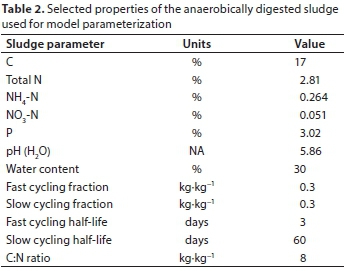
Inorganic fertilizer

The amount and timing of inorganic fertilizer application for this modelling work was based on the Fertilizer Handbook (FSSA, 2007) to meet the target yield for each selected site. The fertilizer was applied at planting and top dressed 5 weeks later according to the FSSA (2007) recommendations presented in Table 3. Limestone ammonium nitrate (LAN) with 28% N content was used as a source of nitrogen to meet the crop N requirement in this study.

 

 

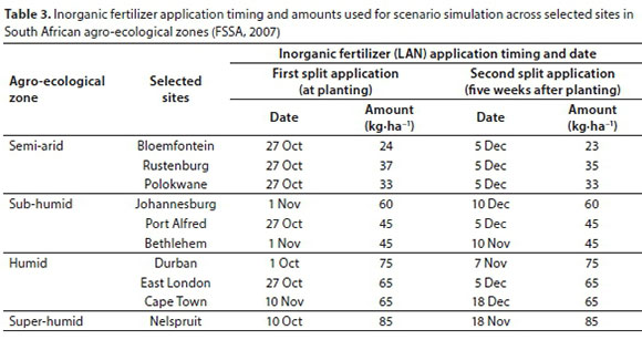
Crop

Maize was selected as test crop because it is one of the most widely cultivated crops across the globe and accounts for 51% of the cultivated land in South Africa (FAO, 2005). A well-studied maize cultivar, PAN 6966, was selected and certain crop model parameters are presented in Table 4.

 

 

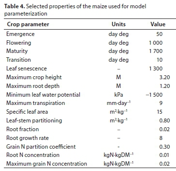
Study site

Scenario simulations were run using the SWB-Sci model for 4 of the 6 major agro-ecological zones of South Africa (Table 5, Column 1) to predict maize grain yield and nitrate leaching from sludge-amended soils using inorganic fertilizer as price benchmark.

The potential yield of maize for the representative sites and inorganic fertilizer recommendations for each site were obtained from FSSA Guidelines (2007) and Du Plessis (2003) (Table 5). Sludge application/recommendation rate was estimated based on the annual sludge N release rates adjusted to match the crop N requirements (Table 5, Column 6) using the SWB-Sci model (Ogbazghi et al., 2015).

Long-term weather records for the selected sites within each agro-ecological zone were obtained from the South African Weather Service (SAWS) for 1993-2013. SAWS collates, maintains and runs a quality control process of South Africa's meteorological and climatological data and related information. This archived data consists of daily rainfall values since 1936 as well as mean hourly and daily data of wind direction, wind speed, temperature, humidity, pressure and sunshine since 1950. Two sites, Nelspruit and Port Alfred, were exceptions, since data were available only for 2002-2013. The annual rainfall figures (1993-2013) of the selected sites are presented in Table 6.

Simulation and statistical analyses conducted

Simulations of 80 scenarios were done based on fully factorial combinations of 4 agro-ecological zones with 3 sites for the semi-arid, sub-humid and humid zones and one for the super-humid zone, and 4 soil textures. Each scenario was run for 20 years of simulation time. The numbers of years were used as replicates, except in testing Hypothesis 2 (that under dryland maize cropping, nitrate leaching and maize grain yield from sludge-amended soils compared with inorganic fertilizer will not vary across seasons at a specific site), where the number of years was used as the main effect. Statistical analyses were done using general linear model (GLM) procedures of Windows SAS version 9.4 (SAS Institute, 2012).

 

RESULTS AND DISCUSSION

Maize grain yield and nitrate leaching across South African agro-ecological zones and sites

Model scenario simulation was carried out to predict maize grain yield and nitrate leaching from sludge-amended soils across 5 of the 6 South African agro-ecological zones. Findings from these model simulation results are presented in the following sections.

Maize grain yield from sludge-amended soils and inorganic fertilizer

Maize grain yield varied significantly across the 4 agro-ecological zones for both sludge and inorganic fertilizer-amended soils (Fig. 1). Generally, maize yield was higher from sludge-amended soils than lands receiving inorganic fertilizer (Fig. 1). The highest average grain yield of 12.6 t∙ha⁻¹ was predicted for the super-humid zone (Nelspruit) under sludge treatment, while lowest yield of 4.1 t∙ha⁻¹ was recorded in the semi-arid zone of Bloemfontein under inorganic fertilizer application. Generally, the predicted yield for the sites was within the ranges reported by FSSA (2007).

 

 

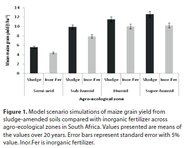
The mean annual maize grain yield varied significantly (P < 0.05) between sites within an agro-ecological zone (Fig. 2). In the sub-humid zone, maize grain yield in Johannesburg was 20% higher under sludge-amended and 32% higher under inorganic fertilizer-amended soils than for Bethlehem. Similarly, in the semi-arid zone, maize grain yield in Rustenburg was 25% higher under sludge-amended and 20% higher under inorganic fertilizer-amended soils than in Bloemfontein. In the humid zone, maize grain yield in Durban was 20% higher under sludge-amended and 28% higher under inorganic fertilizer-amended soils than in East London (Fig. 2). These variations are attributed to the differences in rainfall and temperature between sites, which affected dry matter production and grain yield.

It was apparent from the simulations that maize grain yield from sludge-amended soils varied significantly (P < 0.05) across agro-ecological zones and sites compared with inorganic fertilizer. Maize grain yield was higher from sludge-amended soils than inorganic fertilizer, indicating the agronomic benefits of sewage sludge over inorganic fertilizer.

Nitrate leaching from sludge-amended soils and inorganic fertilizer

Henceforth, the simulation findings showed that nitrate leaching varied significantly (P < 0.05) across agro-ecological zones for both inorganic fertilizer and sludge-amended soils (Fig. 3). Cumulative annual nitrate leaching varied from 11.2 kgNO₃-N∙ha⁻¹ (semi-arid) to 43.2 kgNO₃-N∙ha⁻¹ (super-humid) for inorganic fertilizer-amended soils and from 5.6 kgNO₃-N∙ha⁻¹ (semi-arid) to 32.7 kgNO₃-N∙ha⁻¹ (super-humid) for sludge-amended soils. Generally, nitrate leaching within each agro-ecological zone was significantly higher (P < 0.05) from inorganic fertilizer-amended soils than sludge-amended soils (Fig. 3).

Simulations also showed that nitrate leaching varied between sites within an agro-ecological zone (Fig. 4). For instance, in the semi-arid zone, leaching was higher in Rustenburg (8.1 kgNO₃-N∙ha⁻¹) than in Bloemfontein (4.1 kgNO₃-N∙ha⁻¹) and Polokwane (5.6 kgNO₃-N∙ha⁻¹); in the sub-humid zone, leaching was higher in Johannesburg (34.2 kgNO₃-N∙ha⁻¹) than in Bethlehem (14.2 kg NO₃-N ha⁻¹) and Port Alfred (8.3 kgNO₃-N∙ha⁻¹); and in the humid zone, leaching was higher in Durban (40.2 kgNO₃-N∙ha⁻¹) than in East London (13.2 kgNO₃-N∙ha⁻¹) (Fig. 4).

The variation in nitrate leaching between agro-ecological zones generally follows a similar pattern to the rainfall for both inorganic fertilizer and sludge-amended soils. This concurs with previous findings that reported a direct relationship between water availability and nitrate leaching (Tesfamariam et al., 2015; Holland et al., 2018). Similarly, the difference in nitrate leaching between sites within an agro-ecological zone was attributed mainly to the variation in rainfall amount and distribution. For instance, in the semi-arid zone annual rainfall was 75 mm higher in Rustenburg than Bloemfontein; in the sub-humid zone, rainfall was 80 mm and 60 mm higher in Johannesburg than Bethlehem and Port Alfred; and in the humid zone, rainfall was 150 mm and 134 mm higher in Durban than East London and Cape Town (Tables 5 and 6).

This significant variation between sludge application and inorganic fertilizer was attributed mainly to the form of N. A large fraction of the N in sludge (> 70%) is organic, which is released gradually to plant-available form. In contrast, N in inorganic fertilizers is all inorganic and is potentially leachable under excessive rainfall.

Nitrate losses are low from sludge-amended soils compared with the conventional agronomic use of inorganic fertilizer. For instance, in the semi-arid zone of Rustenburg, only 2.3% of the organic N that is added with sludge was leached, compared with 11.1% for inorganic fertilizer. Similarly, in the sub-humid zone in Johannesburg, 6.2% of the organic N was leached from sludge compared with 28.5%. In the humid zone of Durban 7.9% of the organic N was leached from sludge compared with 26.7%. In the super-humid zone of Nelspruit, only 8.2% of the organic N that is added with sludge was leached as nitrate, compared with 25.4% of inorganic fertilizer. Therefore, using sludge in agricultural lands has a low risk of nitrate leaching compared with inorganic fertilizer. Therefore, the hypothesis that 'under dryland maize cropping, annual maize grain yield and nitrate leaching from sludge-amended soils will remain the same as inorganic fertilizer-amended soil across agro-ecological zones and sites' is not accepted.

 

NITRATE LEACHING AND MAIZE YIELD ACROSS SEASONS

Model scenario simulation was carried out to predict maize grain yield and nitrate leaching from sludge-amended soils across seasons within a site. Findings from these model simulation results are presented in the following sections.

Maize grain yield over years within a site

Model simulations were conducted for over 20 years on 2 selected sites, namely, Johannesburg (sub-humid zone) and Durban (humid zone), to assess maize grain yield from sludge and inorganic fertilizer-amended soils. Maize grain yield varied significantly over years, both for inorganic fertilizer and sludge-treated soils (Fig. 5). Generally, maize grain yield was higher for soils fertilized with sludge than inorganic fertilizer in both Johannesburg and Durban. For instance, in the sub-humid zone of Johannesburg, maize grain yield from sludge-amended soil was predicted to be 10-15% higher than soils amended with inorganic fertilizer (Fig. 5a). Similarly, in the humid zone of Durban, maize grain yield was 15-20% higher in sludge-amended soils than those fertilized with inorganic fertilizer over 20 years (Fig. 5b).

The difference in maize grain yield between years was statistically significant (P < 0.05) when the difference in rain amount between years exceeded 241 mm (semi-arid zone), 362 mm (sub-humid zone), and 429 mm (humid zone). This event happened in 2 of the 20 years (2002 and 2004) of model simulation for both Johannesburg and Durban. Nitrate leaching in these 2 years was also lower compared with other years (Fig. 6). The low rainfall events of 2002 and 2004 led to low grain yield and nitrate leaching, because there is a direct relationship between water availability and maize grain yield (Nilahyane et al., 2019) as well as between high rainfall events and nitrate leaching (Holland et al., 2018). It is well documented that the presence of water plays a critical role in both nutrient uptake by plants and release of nutrients as plant-available inorganic forms from organic nutrient sources (Guntiňas et al., 2012, Ogbazghi et al., 2015).

Nitrate leaching over years within a site

Nitrate leaching varied significantly (P < 0.05) over the years under both sludge and inorganic fertilizer-amended soils (Fig. 6a and 6b). Nitrate leaching remained significantly higher under inorganic fertilizer-amended soils than those that received sludge. For instance, in the sub-humid zone of Johannesburg, the mean annual nitrate leaching from inorganic fertilizer was 15% higher than with sludge-treated soils (Fig. 6a). Similarly, in the humid zone of Durban, the mean annual nitrate leaching from inorganic fertilizer-treated soil was 20% higher than for sludge-treated soil (Fig. 6b). Similar to maize grain yield, the significant difference (P < 0.05) in nitrate leaching between years was observed in 2 of the 20 years.

The observed increase in nitrate leaching as the rainfall increased is attributed to the increase in the mobility of nitrate within the profile, at a relatively faster rate than the rate of uptake by plants. Such interactive effects of both rainfall and leaching on uptake of N by plants are well documented (Banger et al., 2018). Holland et al. (2018) and Ogbazghi et al. (2016) reported a direct relationship between nitrate leaching and soil water availability. Therefore, the hypothesis that 'under dryland maize cropping, annual maize grain yield and nitrate leaching will not vary across years both from sludge and inorganic fertilizer-amended soils' is not accepted.

Maize grain yield and nitrate leaching across soil textures

Maize grain yield and nitrate leaching varied significantly (P < 0.05) between soil textures for both sludge and inorganic fertilizer-amended soils (Fig. 7a and 7b). Maize grain yield was predicted to be higher for clay loam and sandy clay loam soils than for clay and sandy loam soils (Fig. 7a). It was also apparent that maize grain yield was higher from sludge-amended than inorganic fertilizer-amended soil across soil textures (Fig. 7a). This is mainly due to the higher nitrate leaching from inorganic fertilizer compared with sludge-amended soil (Fig. 7b).

Nitrate leaching from inorganic fertilizer-amended soils was generally higher than from sludge-amended soils (Fig. 7b). Nitrate leaching was lower in clay and clay loam soils than in sandy clay loam and sandy loam soils in both sludge and inorganic fertiliser soils. This agrees with the general literature in which nitrate leaching from sand-dominated soils is reported to be higher (Elasbah et al., 2019; Fang and Su, 2019). Therefore, the hypothesis that 'under dryland maize cropping, annual maize grain yield and nitrate leaching will remain similar across soil textures' is not accepted.

 

CONCLUSIONS

Predicted maize grain yield and nitrate leaching varied significantly across 4 agro-ecological zones, for both sludge-amended and inorganic fertilizer-amended soils. Similarly, maize grain yield and nitrate leaching, were predicted to vary significantly across seasons and soil textures for both the sludge- and inorganic fertilizer-amended soils. However, nitrate leaching losses were lower from sludge-amended soils compared with those receiving inorganic fertilizer across all agro-ecological zones. Predicted maize grain yield was higher from sludge-amended soils than for inorganically fertilized crops, while nitrate leaching was higher with inorganic fertilizer than with sludge, indicating the agronomic and environmental benefits of municipal sludge over inorganic fertilizer. Further validation of these findings using field experiments and monitoring potential P accumulation for soils that received sludge according to crop N requirements is recommended.

 

ACKNOWLEDGMENTS

The authors would like to express their appreciation and gratitude to the Water Research Commission of South Africa (WRC) and East Rand Water Care Works (ERWAT) for the funding without which this study would have been but a dream. The authors would like to further express their gratitude to the Agro-Climatology Unit of the South African Agricultural Research Council - Soil, Climate, and Water for providing us with the long-term weather data for the study sites.

 

REFERENCES

ALVAREZ-CAMPOS OM (2019) Assessment of exceptional quality biosolids for urban agriculture. PhD dissertation, Virginia Polytechnic Institute and State University, USA. 145-183.         [ Links ]

ANNANDALE JG, CAMPBELL GS, OLIVIER FC and JOVANOVIC NZ (2000) Predicting crop water uptake under full and deficit irrigation: An example using pea (Pisum sativum L. cv. Puget). Irrig. Sci. 19 65-72. https://doi.org/10.1007/s002710050002        [ Links ]

ANNANDALE J, JOVANOVIC N, CAMPBELL G, SAUTOY ND and BENADE N (2003) A two-dimensional water balance model for micro-irrigated hedgerow tree crops. Irrig. Sci. 22 157-170. https://doi.org/10.1007/s00271-003-0081-7        [ Links ]

BANGER K, NAFZIGER ED, WAND J, MUHAMMAD U and PITTELKOW CM (2018) Simulating nitrogen management impacts on maize production in the U.S. Midwest. PloS ONE 13 10. https://doi.org/10.1371/journal.pone.0201825        [ Links ]

BANGER K, YUAN M, WANG J, NAFZIGER ED and PITTELKOW CM (2017) A vision for incorporating environmental effects into nitrogen management decision support tools for U.S. maize production. Front. Plant Sci. 8 1270. https://doi.org/10.3389/fpls.2017.01270        [ Links ]

BOUNIOLS A, CABELGUENNE M, JONES CA, CHALAMET A, CHARPENTEAU JL and MARTY JR (1991) Simulation of soybean nitrogen nutrition for a silty clay soil in southern France. Field Crops Res. 26 19-34. https://doi.org/10.1016/0378-4290(91)90054-Y        [ Links ]

BRADY NC (1974) The Nature and Property of Soils (8^th edn). Macmillan Publishing Company, Inc., New York, N.Y.         [ Links ]

DU PLESSIS (2003) Maize production. Department of Agriculture, ARC-Grains Crop institute, RSA, URL: www.nda.agric.za/publications.         [ Links ]

ELASBAH R, SELIM T, MIRDAN A, and BERNDTSSON R (2019) Modelling of fertilizer transport for various fertigation scenarios under drip irrigation. Water 11 893. https://doi.org/10.3390/w11050893        [ Links ]

FANG J and SU Y (2019) Effects of soils and irrigation volume on maize yield, irrigation water productivity, and nitrogen uptake. Sci. Rep-UK 9 7740. https://doi.org/10.1038/s41598-019-41447-z        [ Links ]

FAO (2005) Fertilizer use by crop in South Africa. FAO, Rome, Italy.         [ Links ]

FSSA (2007) Fertilizer Handbook (6^th edn). The Fertilizer Society of South Africa. Beria Printers, South Africa. 99-123.         [ Links ]

GODWIN DC and JONES CA (1991) Nitrogen Dynamics in the Soil-Plant Systems. 289-321.         [ Links ]

GUNTIŇAS ME, LEIROS MC, TRASAR-CEPEDA C and GIL-SOTRES F (2012) Effects of moisture and temperature on net soil nitrogen mineralization: A laboratory study. Eur. J. Soil Biol. 48 73-80. https://doi.org/10.1016/j.ejsobi.2011.07.015        [ Links ]

HASSINK J, SCOLEFLED D and BLANTERN P (1990) Nitrogen mineralization in grassland soil. In: Gaborcik N, Krajcovic V and Zimkova M (eds). Proc. 13^th Gen. Meeting of the Eur. Grassland Federation, Banscka Bystrica, Tsjechoslovakia, vol II. 25-32.         [ Links ]

HOLLAND JE, BENNETT AE, NEWTON AC, WHITE PJ, MCKENZIE BM, GEORGE TS, PAKEMAN RJ, BAILEY JS, FORNAR DA and HAYES RC (2018) Liming impacts on soils, crops and biodiversity in the UK: A review. Sci. Total Environ. 610-611 316-332. https://doi.org/10.1016/j.scitotenv.2017.08.020        [ Links ]

KAIKCIOGLU HH and DELIBACAK S (2018) Changes in soil health and crop yield in response to the short-term application of sewage sludge to typic xerofluvent soil in Turkey. Appl. Ecol. Environ. Res. 16 4893-4917. https://doi.org/10.15666/aeer/1604_48934917        [ Links ]

LADD JN, AMATO M, JOCTEUR-MONROZIER L and VAN GESTEL M (1990) Soil microhabitats and carbon and nitrogen metabolism. In: Proc. 14^th Int. Congress Soil Sci., Kyoto, Japan, Vol III. 82-87.         [ Links ]

MALOBANE ME (2014) Using the organic carbon fractions of the Van Soest method to determine compounds responsible for C and N mineralization from sludge amended soils. MSc. dissertation, University of Pretoria, South Africa. 56-64.         [ Links ]

MILES N and MANSON AD (2000) Nutrition of planted pastures. In: Tainton NM (ed.). Pasture Management in South Africa. University of Natal Press, Pietermaritzburg.         [ Links ]

NILAHYANE A, ISLAM MA, MESBAH AO and GARCIA AG (2019) Effect of irrigation and nitrogen fertilization strategies on silage corn grown in semi-arid conditions. Agron 8 208. https://doi.org/10.3390/agronomy8100208        [ Links ]

OGBAZGHI ZM, TESFAMARIAM EH and ANNANDALE JG (2016) Modelling N mineralisation from sludge-amended soils across agro-ecological zones: A case study from South Africa. J. Ecol. Model. 322 19-30. https://doi.org/10.1016/j.ecolmodel.2015.11.019        [ Links ]

PARAMASHIVAM D, DICKINSON NM, CLOUGH TJ, HORSWELL J and ROBINSON BH (2017) Potential environmental benefits from blending biosolids with other organic amendments before application to land. J. Environ. Qual. 43 481-489. https://doi.org/10.2134/jeq2016.10.0421        [ Links ]

RHOADS FM and BENNETT JM (1990) Corn. In: Stewart BA and Nielsen DR (ed.). Irrigation of Agricultural Crops. American Society of Agronomy, Madison, Wis.         [ Links ]

SAS INSTITUTE INC (2012) The SAS system for Windows, Version 9.4., SAS Institute Inc., Cary, NC, USA.         [ Links ]

SCHOEMAN JL and VAN DER WALT M (2004) Agricultural Research Council - Institute for Soil, Climate and Water. Overview of the status of the agricultural natural resources of South Africa. Report No. GW/A/2004/13. ARC-ISCW, Pretoria. 106-118.         [ Links ]

SOIL CLASSIFICATION WORKING GROUP (1991) Soil classification: A taxonomic system for South Africa. Dep. of Agric. Development, Pretoria, South Africa.         [ Links ]

STÖCKLE CO and CAMPBELL GS (1989) Simulation of crop response to water and nitrogen: an example using spring wheat. Trans. ASAE 32 66-68. https://doi.org/10.13031/2013.30964        [ Links ]

STÖCKLE CO, DONATELLI M and NELSON R (2003) CropSyst, a cropping systems simulation model. Eur. J. Agron. 18 289-307. https://doi.org/10.1016/S1161-0301(02)00109-0        [ Links ]

STÖCKLE CO, MARTIN SA and CAMPBELL GS (1994) CropSyst, a cropping systems model: Water/nitrogen budgets and crop yield. Agric. Syst. 46 335-359. https://doi.org/10.1016/0308-521X(94)90006-2        [ Links ]

TESFAMARIAM EH (2009) Sustainable use of sewage sludge as a source of nitrogen and phosphorus in cropping systems. PhD thesis, University of Pretoria, South Africa, pp. 153-159.         [ Links ]

TESFAMARIAM EH, ANNANDALE JG, STEYN JM, STIRZAKER RJ and MBAKWE I (2015) Use of the SWB-Sci model for nitrogen management in sludge-amended land. Agric. Water Manage. 152 262-276. https://doi.org/10.1016/j.agwat.2015.01.023        [ Links ]

TISDALE SL, NELSON WL and BEATON ID (1985) Soil fertility and Fertilizers (4^th edn). Macmillan Publishing Company, New York.         [ Links ]

USEPA (2012) A Plain English Guide to the EPA Part 503 Biosolids Rule. USEPA Rep. 93/003-832. U.S. Gov. Print. Office, Washington, D.C.         [ Links ]

VAN DER LAAN M, STIRZAKER RJ, ANNANDALE JG, BRISTOW KL and DU PREEZ CC (2010) Monitoring and modelling draining and resident soil water nitrate concentrations to estimate leaching losses. Agric. Water Manage. 97 1779-1786. https://doi.org/10.1016/j.agwat.2010.06.012        [ Links ]

VERBERNE ELJ, HASSINK J, DE WILLIGEN P, GROOT JJR and VAN VEEN JA (1990) Modelling organic matter dynamics in different soils. Neth. J. Agric. Sci. 38 221-238.         [ Links ]

ZHAO H, LI X, and JIANG Y (2019) Response of nitrogen losses to excessive nitrogen fertilizer application in intensive greenhouse vegetable production. Sustainability 11 1513. https://doi.org/10.3390/su11061513        [ Links ]

 

 

Received 4 April 2018
Accepted in revised form 20 September 2019

 

 

* Corresponding author, email: eyob.tesfamariam@up.ac.za

^rND^sANNANDALE^nJG^rND^sCAMPBELL^nGS^rND^sOLIVIER^nFC^rND^sJOVANOVIC^nNZ^rND^sANNANDALE^nJ^rND^sJOVANOVIC^nN^rND^sCAMPBELL^nG^rND^sSAUTOY^nND^rND^sBENADE^nN^rND^sBANGER^nK^rND^sNAFZIGER^nED^rND^sWAND^nJ^rND^sMUHAMMAD^nU^rND^sPITTELKOW^nCM^rND^sBANGER^nK^rND^sYUAN^nM^rND^sWANG^nJ^rND^sNAFZIGER^nED^rND^sPITTELKOW^nCM^rND^sBOUNIOLS^nA^rND^sCABELGUENNE^nM^rND^sJONES^nCA^rND^sCHALAMET^nA^rND^sCHARPENTEAU^nJL^rND^sMARTY^nJR^rND^sELASBAH^nR^rND^sSELIM^nT^rND^sMIRDAN^nA^rND^sBERNDTSSON^nR^rND^sFANG^nJ^rND^sSU^nY^rND^sGUNTIŇAS^nME^rND^sLEIROS^nMC^rND^sTRASAR-CEPEDA^nC^rND^sGIL-SOTRES^nF^rND^sHASSINK^nJ^rND^sSCOLEFLED^nD^rND^sBLANTERN^nP^rND^sHOLLAND^nJE^rND^sBENNETT^nAE^rND^sNEWTON^nAC^rND^sWHITE^nPJ^rND^sMCKENZIE^nBM^rND^sGEORGE^nTS^rND^sPAKEMAN^nRJ^rND^sBAILEY^nJS^rND^sFORNAR^nDA^rND^sHAYES^nRC^rND^sKAIKCIOGLU^nHH^rND^sDELIBACAK^nS^rND^sLADD^nJN^rND^sAMATO^nM^rND^sJOCTEUR-MONROZIER^nL^rND^sVAN GESTEL^nM^rND^sMILES^nN^rND^sMANSON^nAD^rND^sOGBAZGHI^nZM^rND^sTESFAMARIAM^nEH^rND^sANNANDALE^nJG^rND^sPARAMASHIVAM^nD^rND^sDICKINSON^nNM^rND^sCLOUGH^nTJ^rND^sHORSWELL^nJ^rND^sROBINSON^nBH^rND^sRHOADS^nFM^rND^sBENNETT^nJM^rND^sSTÖCKLE^nCO^rND^sCAMPBELL^nGS^rND^sSTÖCKLE^nCO^rND^sDONATELLI^nM^rND^sNELSON^nR^rND^sSTÖCKLE^nCO^rND^sMARTIN^nSA^rND^sCAMPBELL^nGS^rND^sTESFAMARIAM^nEH^rND^sANNANDALE^nJG^rND^sSTEYN^nJM^rND^sSTIRZAKER^nRJ^rND^sMBAKWE^nI^rND^sVAN DER LAAN^nM^rND^sSTIRZAKER^nRJ^rND^sANNANDALE^nJG^rND^sBRISTOW^nKL^rND^sDU PREEZ^nCC^rND^sVERBERNE^nELJ^rND^sHASSINK^nJ^rND^sDE WILLIGEN^nP^rND^sGROOT^nJJR^rND^sVAN VEEN^nJA^rND^sZHAO^nH^rND^sLI^nX^rND^sJIANG^nY^rND^1A01 A02^nZama Eric^sMashimbye^rND^1A01^nWillem Petrus^sDe Clercq^rND^1A02^nAdriaan^sVan Niekerk^rND^1A01 A02^nZama Eric^sMashimbye^rND^1A01^nWillem Petrus^sDe Clercq^rND^1A02^nAdriaan^sVan Niekerk^rND^1A01 A02^nZama Eric^sMashimbye^rND^1A01^nWillem Petrus^sDe Clercq^rND^1A02^nAdriaan^sVan Niekerk

RESEARCH PAPERS

 

Assessing the influence of DEM source on derived streamline and catchment boundary accuracy

 

 

Zama Eric Mashimbye^{I, II, *}; Willem Petrus De Clercq^I; Adriaan Van Niekerk^II

^IDepartment of Soil Science, Stellenbosch University, Private Bag X1, Matieland 7602, South Africa
^IIDepartment of Geography and Environmental Studies, Stellenbosch University, Private Bag X1, Matieland 7602, South Africa

 

 

---

ABSTRACT

Accurate DEM-derived streamlines and catchment boundaries are essential for hydrological modelling. Due to the popularity of hydrological parameters derived mainly from free DEMs, it is essential to investigate the accuracy of these parameters. This study compared the spatial accuracy of streamlines and catchment boundaries derived from available digital elevation models in South Africa. Two versions of Stellenbosch University DEMs (SUDEM5 and DEMSA2), the second version of the 30 m advanced spaceborne thermal emission and reflection radiometer global digital elevation model (ASTER GDEM2), the 30 and 90 m shuttle radar topography mission (SRTM30 and SRTM90 DEM), and the 90 m Water Research Commission DEM (WRC DEM) were considered. As a reference, a 1 m GEOEYE DEM was generated from GeoEye stereo images. Catchment boundaries and streamlines were extracted from the DEMs using the Arc Hydro module. A reference catchment boundary was generated from the GEOEYE DEM and verified during field visits. Reference streamlines were digitised at a scale of 1:10 000 from the 1 m orthorectified GeoEye images. Visual inspection, as well as quantitative measures such as correctness index, mean absolute error, root mean squares error and figure of merit index were used to validate the results. The study affirmed that high resolution (<30 m) DEMs produce more accurate parameters and that DEM source and resampling techniques also play a role. However, if high resolution DEMs are not available, the 30 m SRTM DEM is recommended as its vertical accuracy was relatively high and the quality of the streamlines and catchment boundary was good. In addition, it was found that the novel Euclidean distance-based MAE and RMSE proposed in this study to compare reference and DEM-extracted raster datasets of different resolutions is a more reliable indicator of geometrical accuracy than the correctness and figure of merit indices.

Keywords: hydrology, catchment delineation, digital elevation model, correctness index, figure of merit index, Euclidean distance index

---

 

 

INTRODUCTION

Digital elevation model (DEM) derived catchment boundaries, sub-basins and streamlines play an important role in hydrological studies (Li and Wong, 2010; Martz and De Jong, 1998; O'Callaghan and Mark, 1984; Renssen and Knoop, 2000; Turcotte et al., 2001; Vogt et al., 2003). The availability of good quality DEMs makes it possible to carry out hydrological and geomorphological analyses on regional or national levels (Moore and Wilson, 1992; Thomas et al., 2014). DEMs are offered at a variety of resolutions ranging from very high (0.1-5 m) to low (1 km) (Behrens et al., 2010; Tarekegn et al., 2010). Very high resolution (VHR) DEMs, as derived from airborne light detection and ranging (LiDAR) data, are often only available for small areas, particularly in developing countries where this technology is still prohibitively expensive. Consequently, freely available near-global DEMs are frequently used for hydrological studies at national or regional scales.

Various studies have investigated the value of DEMs for hydrological analysis. For instance, Weepener et al. (2012) developed a hydrologically improved DEM for South Africa from the SRTM90 DEM using 20 m 1:50 000 contours and ASTER GDEM data. They found that useful river lines and catchment boundaries can be delineated from the hydrologically improved SRTM90 DEM. Li and Wong (2010) compared stream networks extracted from the national elevation dataset (NED), SRTM90 DEM and LiDAR with stream networks extracted from the national hydrography dataset (NHD). They also compared flood simulations using the stream networks delineated from the different DEMs and concluded that higher-resolution DEMs can derive more accurate river networks, but that the spatial resolution of a DEM only has a minor effect on flood simulation results. Callow et al. (2007) evaluated the effect of commonly used hydrological correction methods (stream burning, Agree, ANUDEM v4.6.3 and ANUDEM v5.1) on the overall nature of a DEM. They found that different methods produce non-convergent results for catchment boundaries, stream position and length, and that these techniques differentially compromise secondary terrain analysis. Their study also concluded that, while hydrological correction methods successfully improved the calculation of the catchment area, stream position and length, they increased catchment slope.

DEMs invariably contain errors, most of which can be attributed to the data source, methods, topography complexity and spatial resolution (Aguilar et al., 2005; Kinsey-Henderson and Wilkinson, 2013; Mukherjee et al., 2011; Mukherjee et al., 2013; Thomas et al., 2014; Rodriguez et al., 2005). It has also been reported that the accuracy of a DEM is dependent on its application (Sharma and Tiwari, 2014; Sharma et al., 2010). Kensey-Henderson and Wilkinson (2013) compared DEMs derived from synthetic aperture radar (SAR) data and DEMs interpolated from topographical data for slope gradient and soil erosion estimation in low relief areas. They evaluated the magnitude of error in DEM slope and erosion estimates using the Revised Universal Soil Loss Equation. They determined that the SRTM DEMs provided more accurate estimates of slope gradient and erosion in low relief areas.

Frey and Paul (2012) investigated the suitability of the SRTM90 DEM and the ASTER GDEM for the compilation of glacier-specific topographic parameters in Switzerland. Comparing the delineated parameters with those derived from the Swiss national DEM (DHM25), they concluded that, although the SRTM90 DEM yielded slightly more accurate results, both DEMs were suitable for the compilation of topographic parameters in glacier inventories.

Evidently, the freely available medium (90 m) and high resolution (30 m) near-global DEMs have opened up many possibilities for hydrological analyses, especially at national and regional scales (De Clercq et al., 2013; Wang et al., 2011; Weepener et al., 2012; Sharma and Tiwari, 2014). Researchers frequently use these DEMs for hydrological studies, mainly because they are freely available (De Clercq et al., 2013; Gichamo et al., 2012; Wang et al., 2011; Weepener et al., 2012). However, little attention has been paid to the quality of the products that are derived from these DEMs. Given their popularity, it is important to assess the accuracy of the derived hydrological parameters so that uncertainties can be considered in the interpretation of hydrological analysis results. For South Africa, in addition to the freely available global DEMs (for example, SRTM and ASTER GDEM), a hydrologically improved Water Research Commission (WRC) DEM is available. While these DEMs are widely used to derive hydrological parameters, the accuracy of the resultant parameters has not been evaluated. This study investigated the validity of hydrological parameters derived from these freely available DEMs. The spatial accuracy of catchment boundaries and streamlines derived from a total of 7 DEMs that are available at national level in South Africa was evaluated. In addition, this study investigated a novel Euclidean distance-based technique for validating the geometric accuracy of DEM derived streamlines and catchment boundaries using root mean squares error and mean absolute error.

 

MATERIAL AND METHODS

The study site

The study area is the Sandspruit catchment, a subcatchment of the Berg River in the Western Cape Province, South Africa (Fig. 1). The catchment is located in a winter rainfall region, and the mean annual rainfall is about 400 mm (Flügel, 1995). The study area is 152 km² in size and has a gently hilly topography. The geology of the Sandspruit catchment is mainly Malmesbury shales, even though there are smaller occurrences of fine sediment, silcrete-ferricrete, greenstone, quartzite and granite. An opencast mine is located in the south-eastern part of the catchment. While the catchment is largely used for dryland cultivation of winter wheat, canola and pasture are also cultivated, and a small proportion of the catchment is covered by natural vegetation.

Datasets used

The datasets used in this study included trig beacon heights, field survey points, satellite and aerial imagery, DEMs, reference streamlines and a reference catchment boundary. Each of these datasets is described in the following subsections.

Trig beacons and field survey points

A combination of trig beacons and GPS field survey points were used to validate the vertical accuracy of the DEMs. Trig beacons covering the Sandspruit catchment, established by the South African Chief Directorate of National Geo-spatial information (CDNGI) and their coordinates (including ground height), were obtained from the Centre for Geographical Analysis (CGA) at Stellenbosch University. GPS field survey points were measured using a survey grade Trimble Differential GPS. The GPS points were differentially corrected to improve their accuracy to about 10 cm. A total of 38 points (6 trig beacons and 32 GPS points) were used as reference points to validate the DEMs.

Satellite and aerial imagery

GeoEye stereo-images were acquired from Geo Data Design. The 0.4 m resolution images were captured in July 2011, a period in the year when crops in the study area were still at seedling height. Vegetation would therefore have had a minimal effect on photogrammetrically extracted heights.

Very high-resolution (0.5 m) orthorectified digital aerial images covering the study area were sourced from CDNGI (http://www.ngi.gov.za). The images were acquired in 2007 and were used as spatial reference during the orthorectification of GeoEye stereo images.

DEMs

The DEMs considered in this study were the SRTM90 DEM, SRTM30 DEM, ASTER GDEM2, two versions of Stellenbosch University's digital elevation model (SUDEM) (SUDEM5 and the digital elevation model of South Africa), the 90 m Water Research Commission DEM (WRC DEM) and a 1 m DEM generated from GeoEye images (GEOEYE DEM).

The SRTM90 DEM was completed in 2000 and provides the first medium-resolution DEM data at near-global scale (Farr and Kobrick, 2001; Li and Wong, 2010). The SRTM90 DEM has an absolute vertical error of less than 16 m and an absolute horizontal accuracy of 20 m (Farr, 2000; Mulder et al., 2011; Van Niekerk, 2008). According to the Consultative Group on International Agricultural Research Consortium for Spatial Information (CGIAR-CSI, 2011), the SRTM DEM data have been processed to fill data voids and can be used by a wide range of potential users.

The SRTM30 DEM is a near-global DEM that comprises a combination of data from the Shuttle Radar Topography Mission flown in February 2000 and the United States Geological Survey's GTOPO30 data set (USGS, 2016).

The ASTER GDEM was developed jointly by the Ministry of Economy, Trade and Industry (METI) of Japan and the United States National Aeronautics and Space Administration (NASA). The second version of ASTER GDEM (GDEM2) was released in October 2011 (ASTER GDEM Validation Team, 2011) with the inclusion of 26 000 additional scenes to improve coverage. The new version uses a smaller correlation kernel to yield higher spatial resolution, and water masking was also enhanced. ASTER GDEM2 was validated by comparing it to the absolute geodetic references over the conterminous United States (CONUS), the national elevation grids over the US and Japan, the SRTM 1 arc-second DEM over the US and 20 sites around the globe, and global space-borne laser altimeter data. The vertical and horizontal accuracy of the GDEM2 is estimated at 17 m and 71 m, respectively (ASTER GDEM Validation Team, 2011; Mukherjee et al., 2013).

The SUDEM, developed by the Centre for Geographical Analysis (CGA) at Stellenbosch University, is a commercially available product. As of 2015, four products that involve various levels of processing were produced (Van Niekerk, 2016). The 5 m resolution SUDEM5 was generated by fusing the 30 m SRTM DEM with the so called 'Level 1 product'. The Level 1 product (5 m spatial resolution) was interpolated from large (1:10 000) and smaller (1:50 000) scale contours and spot-height data (Van Niekerk, 2016). Smaller-scale contours were only used in areas where large-scale data were not available. Using LiDAR data as reference, the SUDEM5 product was estimated to have a mean absolute error (MAE) of 2.2 m (Van Niekerk, 2016). The 2 m digital elevation model of South Africa (DEMSA2) is a digital surface model (DSM) that is available at 2 m resolution. This DEM was extracted from 0.5 m resolution CDNGI stereo aerial photography (Van Niekerk, 2016). Based on surveyed reference points, the MAE of DEMSA2 product is estimated to be 0.35 m (Van Niekerk, 2016). The SUDEM and DEMSA2 products were considered in this study as they are the only very high resolution DEMs available nationally in South Africa.

The Water Research Commission's digital elevation model (WRC DEM) was developed by the Agricultural Research Council (ARC) for the WRC (Weepener et al., 2012). This DEM was interpolated from the SRTM90 DEM. The SRTM voids were filled with elevation values interpolated from 20 m (1:50 000 scale) vertical interval contours obtained from CDNGI. The resulting DEM was hydrologically corrected by filling sinks and depressions. The vertical accuracy of the WRC DEM was determined to be less than 5 m.

The GEOEYE DEM was created from GeoEye stereo images acquired in July 2011 using the rational polynomial coefficients (RPC) model in the LPS module of ERDAS Imagine software (www.intergraph.com). The GEOEYE DEM was extracted at 1 m horizontal intervals and was validated using reference points (trigonometric beacons) in the Sandspruit catchment. A MAE of 0.70 m was recorded. The GEOEYE DEM was used to delineate a reference catchment boundary. The reference catchment boundary was extracted using the Arc Hydro module in ArcGIS 10.

Reference catchment boundary and reference streamlines

Reference streamlines were digitised at a scale of 1:10 000 from the 1 m orthorectified GeoEye images. The reference streamlines were visually compared to the 1:50 000 national riverlines dataset. It was found that, although the two datasets were geometrically aligned, the 1:50 000 streamlines were much more generalised and contained many topological errors (e.g. gaps).

The reference catchment boundary, generated from the 1 m resolution GEOEYE DEM, was used to validate the lower resolution DEM-delineated catchment boundaries. The reference catchment boundary was validated during several field visits and by visual inspection in ERDAS Stereo Analyst (www.intergraph.com).

Delineation of catchment boundaries and streamlines from DEMs

The Arc Hydro extension for ArcGIS software was used to delineate the Sandspruit catchment boundaries and streamlines from the DEMs. All the datasets were projected to the Universal Transverse Mercator (UTM) coordinate system (Zone 34S). Catchment boundaries and streamlines were extracted at the native resolution of the DEMs. Additionally, the DEMs were resampled to the resolution of the coarsest DEMs (90 m) to allow comparison without the effect of spatial resolution. The threshold for stream delineation was set at 1% of the maximum flow accumulation, as recommended by Arc Hydro's rule of thumb for stream delineation from DEMs (Merwade, 2012; Tarboton, 2003). The GEOEYE DEM was used to calculate reference flow accumulation thresholds for the other DEMs at their respective resolutions. For catchment boundary delineation, outlet (pour) points were selected at the same position. A stream network was extracted from the GEOEYE DEM to enable comparison with previous studies conducted with very high resolution (VHR) DEMs (Li and Wong, 2010). Catchment boundaries and streamlines extracted from all the DEMs were converted to raster datasets using the Feature to Raster tool in ArcGIS 10.1, and the cell size was set to 5 m for comparison purposes. Cells representing boundaries or streamlines (using the GRID_CODE ID of the feature dataset generated by Arc Hydro) were allocated values of 1. All other cells were defined as having no values (i.e. NODATA). Separate raster datasets were created for catchment boundaries and streamlines.

Validation

Vertical accuracy of the DEMs

The vertical accuracies of the DEMs were determined using the absolute and relative mean error (MAE), absolute and relative root mean squares error (RMSE) and 90^th percentile, based on a combination of trig beacons and differentially corrected GPS points as a reference. RMSE, MAE and 90^th percentile are metrics based on reference values commonly used to determine the accuracy of a DEM (Rawat et al., 2019). The MAE and RMSE were calculated based on Eqs 1 and 2:

where X_i is the elevation of a DEM at point i, Y_i is the reference elevation at point i, and n is the number of samples. According to Rawat et al. (2019), RMSE varies with the variability within the distribution of error magnitudes, square root of the number of errors and the magnitude of MAE. MAE is a more natural measure of average error and, unlike RMSE, is unambiguous (Rawat et al., 2019). Lower RMSE and MAE values show good accuracy. The 90^th percentile error reveals the value below which 90% of the errors fall.

DEM delineated catchment boundaries and streamlines

The catchment boundaries and streamlines extracted from the DEMs were visually compared to the reference datasets. Four measures, namely the correctness index (C_r), figure of merit index (FMI), MAE and RMSE were used to quantitatively evaluate continuous delineated catchment boundaries and stream networks. The C_r and FMI were introduced by Li and Wong (2010) to validate stream networks extracted from DEMs, while MAE and RMSE are proposed in this study as additional measures of spatial agreement.

The C_r compares two sets of raster cells (A and B), which represent DEM-extracted and reference raster datasets, respectively (Li and Wong, 2010). The C_r is calculated by Eq. 3 below:

where N_B is the number of cells representing the reference raster and N_(A∩B) is the number of cells of the DEM-extracted raster. Index values range between 0 and 1, and indicate the proportion of the reference raster that is correctly represented by the extracted raster (Li and Wong, 2010). A high correctness index value indicates a high accuracy of extracted streams.

According to Li and Wong (2010), C_r does not reflect how well the extracted raster (representing stream networks in their case) can reproduce the entire actual raster, and they assert that the FMI offers a better solution. The FMI is the ratio of the intersection of the observed change and predicted change to the union of observed change and predicted change (Pontius et al., 2008; Perica and Foufoula-Georgiou, 1996). FMI is computed by Eq. 4 below:

where N_(A∩B) is the number of unique cells found in rasters A and B and N_(A∩B) is the total number of cells found in both A and B (overlapping cells are only counted once). FMI values range between 0 and 1, and a higher FMI value indicates a higher overlap between the two raster datasets, therefore high accuracy.

Euclidean distance (ED) is calculated from the centre of the reference raster cell to the centre of the extracted raster cell. Figure 2 depicts how ED is calculated for streamlines. MAE and RMSE consider the offset (ED) between cells in the reference raster and the closest cell in the candidate raster. The sum of the offsets was used to calculate MAE and RMSE using Eqs 1 and 2. Relatively low MAE and RMSE values indicate a high accuracy of DEM-extracted raster datasets. RMSE is considered a better indicator of accuracy as it is more sensitive to outliers than MAE, but it is often useful to interpret these measures in combination. Large differences between MAE and RMSE are indicative of high variances in individual errors (i.e. outliers).

 

 

RESULTS

Vertical accuracy of the DEMs

The descriptive and accuracy statistics of all the DEMs used in this study are given in Table 1 and Fig. 3. The DEMs show disparities in how they represent the character of the study area, as depicted by the variances in the different descriptive and accuracy measures recorded (Table 1, Fig. 3). ASTER GDEM2 shows the highest bias followed by the SRTM30 and SRTM90, GEOEYE DEM, WRC DEM, DEMSA2 and SUDEM5 (Fig. 3). The absolute and relative MAE and RMSE are <1.54 m for DEMSA2, <3.28 for SUDEM5, <3.75 for GEOEYE DEM, <6.99 for SRTM30 DEM, <7.14 for WRC DEM, <12.35 for ASTER GDEM2 and >13.03 for SRTM90 DEM, respectively. Regarding the 90^th percentile, 90% of elevation values fall below 2.17 (DEMSA2), 2.28 (SUDEM5), 3.09 (GEOEYE DEM), 7.37 (SRTM30 DEM), 9.05 (WRC DEM), 12.3 (ASTER GDEM2) and 12.99 (SRTM90), respectively. It is obvious that DEMSA2 is the most accurate (vertically), followed by SUDEM5, GEOEYE DEM, SRTM30 DEM, WRC DEM, ASTER GDEM2 and SRTM90 DEM.

DEM-delineated catchment boundaries

Based on visual assessment, the catchment boundaries extracted from all the DEMs seem relatively accurate compared to the reference catchment boundary (see Fig. 4a-f). It appears that SUDEM5 and DEMSA2 delineated very accurate catchment boundaries (Fig. 4e, f). The catchment boundaries delineated from these DEMs show small discrepancies with the reference catchment boundary. While the catchment boundaries delineated from the SRTM30 DEM and WRC DEM also appear to be visually accurate, the discrepancies of the catchment boundaries delineated from these DEMs seem slightly greater than those of the SUDEM5 and DEMSA2 (Fig. 4b, d). The WRC DEM appears to delineate a better boundary than the SRTM30 DEM at the area occupied by a mine on the south-eastern part of the Sandspruit catchment (Fig. 4b, d). The ASTER GDEM2 and SRTM90 DEM delineated catchment boundaries show visibly larger discrepancies with the reference catchment boundary (Fig. 4a, c). While the ASTER GDEM2 shows a large discrepancy with the reference catchment boundary in the middle of the eastern part of the catchment, the SRTM90 DEM catchment boundary shows a larger discrepancy compared to the reference boundary in the vicinity of the mine at the south-eastern part of the catchment and at the outflow of the catchment at the north-eastern part. The SRTM90 DEM appears to overestimate the catchment boundary in the south-eastern parts, but performs better than the ASTER DEM2 in delineating the eastern boundary (Fig. 4c). The ASTER GDEM2 slightly underestimates the catchment boundary at the south-eastern part of the catchment and is also unable to correctly delineate the eastern boundary (Fig. 4c).

Regarding the accuracy measures at the supply resolution of the DEMs, DEMSA2 yielded the lowest RMSE and MAE, followed by SUDEM5, SRTM30 DEM, ASTER GDEM2, WRC DEM and the SRTM90 DEM (Fig. 5). The C_r and FMI ratios for SUDEM5 and DEMSA2 are all at near-maximum values (C_r = FMI = 0.99). Whereas the C_r values for SRTM30 DEM and WRC DEM are near maximum and equal (C_r = 0.99), the FMI ratio for SRTM30 DEM is slightly higher than that of WRC DEM (Fig. 5). The ASTER GDEM2 recorded the lowest C_r and FMI values. From these results, it is clear that DEMSA2 delineated the most accurate catchment boundary followed by the SUDEM5 (Fig. 5). Figure 5 indicates that the SRTM30 DEM yields a more accurate catchment boundary in comparison to the ASTER GDEM2. When comparing the medium resolution (MR) DEMs, it is clear that the WRC DEM delineated a more accurate boundary than the SRTM90 DEM (Fig. 5). While the vertical accuracy of DEMSA2, SUDEM5, SRTM30 DEM and SRTM90 DEM is in line with the accuracy of the delineated catchment boundary, this is not the case for ASTER GDEM2 and WRC DEM. Although the WRC DEM yielded a better vertical accuracy than the ASTER GDEM2, the ASTER GDEM2 delineated a slightly more accurate catchment boundary than the WRC DEM (Table 1 and Fig. 3, Fig. 5). Based on the differences between RMSE and MAE, it is obvious that VHR DEMs yielded lower variations in individual errors and that accuracy decreased as resolution decreased (Fig. 5). As can be seen in Fig. 5, the variation in individual errors for catchment delineation increases with an increase in the spatial resolution of the DEMs.

For catchment delineation performed when all DEMs are resampled to MR, SRTM30 DEM records the lowest RMSE, followed by DEMSA2, WRC DEM, SUDEM5, ASTER GDEM2 and SRTM90 DEM (Fig. 6). With regard to MAE, WRC DEM yields the lowest MAE values, followed by DEMSA2, SUDEM5, SRTM30 DEM, ASTER GDEM2 and SRTM90 DEM (Fig. 6). Similarly, lower Cr and FMI values for catchment delineation are seen when the DEMs are resampled to MR (Fig. 6). For the VHR DEMs, DEMSA2 delineates a more accurate catchment boundary than SUDEM5 as was the case at supply resolutions. A similar trend is observed for the HR DEMs and the MR DEMs where SRTM 30 DEM delineates a better boundary than ASTER GDEM2. It is obvious from Fig. 6 that the variations in individual errors for the VHR and HR DEMs for catchment boundary delineation increase when they are resampled to MR. The variations in individual errors for SRTM30 DEM and WRC DEM are lower than those of very high resolution DEMs (DEMSA2 and SUDEM5) when they are resampled to MR.

DEM-extracted streamlines

Streamlines extracted from the DEMs are depicted in Fig. 7a-g. Visually, the streamlines appear to align well with the reference streamlines, although some misalignments for the different DEMs are apparent in certain areas. An in-depth view of a selected area around the mid-northern part of the catchment reveal larger discrepancies for the GEOEYE DEM, ASTER GDEM2 and the SRTM30 DEM (Fig. 7a, b and c). The visual discrepancies of the streams delineated from the SRTM90 DEM, WRC DEM and SUDEM5 appear to be smaller than those of GEOEYE DEM, ASTER GDEM2 and the SRTM30 DEM. Visually, the DEMSA2 streams align very well with the reference streamlines (Fig. 7g).

At DEM supply resolution, GEOEYE DEM recorded the longest streamlines, followed by SUDEM5, DEMSA2, ASTER GDEM2, SRTM30 DEM, WRC DEM and SRTM90 DEM (Fig. 8). The RMSE and MAE values for delineated streamlines for all the DEMs are similar. Similarly, the variation of individual errors for stream delineation for the DEMs is similar for all the DEMs (Fig. 8). C_r and FMI values for all DEMs are low. VHR DEMs recorded slightly larger C_r and FMI values.

 

 

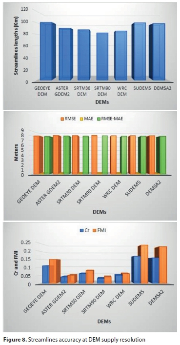
Regarding delineation when the finer resolution DEMs are resampled to MR, the total lengths of extracted streamlines are generally shorter for all DEMs, with the exception of ASTER GDEM2. Contrary to streamline lengths extracted at supply resolution, ASTER GDEM recorded the longest streamlines, followed by DEMSA2, GEOEYE DEM, SUDEM5, WRC DEM, SRTM30 DEM and SRTM90 DEM. As at DEM supply resolution, RMSE and MAE for delineated streamlines are similar for all the DEMs (Fig. 9). It does not seem that the geometric accuracy of the DEM extracted streamlines is in line with the vertical accuracy of the DEMs (Table 1 and Fig. 3, Fig. 9).

 

 

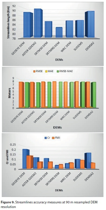
DISCUSSION

All the DEMs used in this study show reliable vertical accuracies. The overall vertical accuracies of DEMSA2 and SUDEM5 are slightly lower than reported by Van Niekerk (2016). This is likely due to the use of a combination of differentially corrected GPS points and trig beacon heights in this study, whereas LiDAR data were used by Van Niekerk (2016). Also, validation data used in this study were mainly biased along the main channel in the catchment. Although the surveyed points were mainly measured on areas without vegetation, it is likely that riparian vegetation could have influenced the accuracy as it could have been included in the pixels. The vertical accuracies of SRTM DEM and ASTER GDEM2 are higher than reported in product specifications. While the absolute vertical accuracy of SRTM DEM and ASTER GDEM2 were reported to be around 16 m and 17 m, respectively, all vertical accuracy measures used in this study yielded accuracy values <14 m for both DEMs. These results are consistent with previous findings where Elkhrachy (2018) reported absolute vertical accuracies of 5.94 and 5.07 m for the SRTM30 DEM and ASTER GDEM2, respectively. Also, Patel et al. (2016) recorded absolute RMSE values of 3.72 and 6.03 m for the SRTM30 DEM and ASTER GDEM2, respectively. The vertical accuracy of WRC DEM is consistent with what was reported by Weepener et al. (2012). The vertical accuracy of GEOEYE DEM is slightly less than that of SUDEM5 and DEMSA2. Occurrence of vegetation could have influenced the accuracy of the GEOEYE DEMs since the survey was conducted in August 2017 whilst the stereo images used to create the DEM were captured in July 2011. Areas without vegetation along the stream could easily have been vegetated by the time the imagery was taken.

Reliable catchment boundaries were delineated from VHR to medium-resolution DEMs investigated in this study when carried out at supply resolutions. Based on the assessment indicators, the VHR DEMs yielded more accurate catchment boundaries followed by high-resolution and medium-resolution DEMs at supply resolution. DEMSA2 demonstrates superiority over all the DEMs for catchment delineation, while the SUDEM5 also records a relatively accurate catchment boundary at supply resolution. While SRTM30 DEM yielded a more accurate catchment boundary than ASTER GDEM2 at supply resolution for the HR DEMs, the WRC DEM recorded a more reliable boundary in comparison to the SRTM90 DEM for MR DEMs. DEM resolution does not appear to play any role when catchment boundaries are extracted at medium resolution for all the DEMs. These findings are consistent with previous studies that demonstrated that the outputs of hydrological modelling are not influenced by DEM resolution alone (Tan et al., 2015; Wang et al., 2015; Wang et al., 2011; Wu et al., 2008; Chaplot, 2005; Wolock and Price, 1994), as the DEM source (Wang, Yang and Yao, 2011; Li and Wong, 2010) and resampling technique (Wu et al., 2008) also play a role in the accuracy of delineated hydrological parameters. According to Woodrow et al. (2016), Zhang et al. (2008), Garbrecht and Martz (2000) and Walker and Willgoose (1999), the source of data used to generate a DEM is the main factor determining the spatial and horizontal detail of a DEM. DEMs derived from contours and spot heights are known to be generalized and are unlikely to contain sufficient detail in areas where the horizontal contour interval is larger than the DEM resolution (Vaze et al., 2010).

In this study, a catchment with relatively moderate terrain was chosen to assess the quality of the derived datasets. It is expected that the quality of the SUDEM5 products will improve as terrain complexity increases, as they are largely unaffected by distortions caused by view angle and vegetation cover. Contours are also more densely distributed in areas of complex terrain, which means that interpolated elevations are generally more accurate in such areas. The better performance of the SRTM 30 DEM in comparison to ASTER GDEM for catchment delineation is in line with the findings of Li et al. (2013) who investigated the impact of resolution and DEM source based on ASTER GDEM and SRTM90 DEM and found that SRTM DEM performed better than ASTER GDEM, irrespective of the course grid size. Also, Zhang et al. (2008) evaluated SRTM, NED and LiDAR DEMs at three spatial resolutions (4, 10 and 30 m) in simulating hydrologic responses. They concluded that a 10 m LiDAR DEM recorded the best results.

With regard to delineation performed when VHR and HR DEMs are resampled to MR, the accuracy of the catchment boundaries decreases substantially. This is likely due to the resampling technique. Le Coz et al. (2009) used 6 resampling techniques to aggregate the SRTM DEM from 0.09 to 10 km. They found that mean and median resampling techniques yielded smoother relief while maximum and nearest neighbour produced rougher relief, which resulted in overestimation of the surface area of floodplains. A nearest neighbour resampling techniques was used in this study.

Similar to catchment boundary delineation, reliable streamlines were extracted from all DEMs used in this study. The accuracy of streamlines extracted from all the DEMs appears to be similar irrespective of resolution and the vertical accuracy of DEMs. While the differences in the accuracy measures are slight, they do not seem to be in line with the resolutions and vertical accuracies of the DEMs. This is in contrast to Charrier and Li (2012), who found that the offset from the reference tends to continuously increase as DEM resolution decreases. Vogt et al. (2003) also demonstrated that the quality of DEM-derived river networks is limited by the spatial resolution and vertical accuracy of the underlying DEMs. However, our study is in support of Charrier and Li (2012) with respect to the length of streamlines decreasing with decreasing DEM resolutions, and that the mean offset is mainly less than the cell size of the DEMs. In this study, the offset is similar for all the DEMs. It is likely that terrain complexity affects the delineation of streamlines in the current study. The studied catchment has moderate terrain. For streamline delineation at HR, the SRTM30 DEM performed better compared to the ASTER GDEM2. According to Tarekegn et al. (2010), ASTER-based DEMs are relatively accurate in near-flat and smoothly-sloped areas, but they are characterised by large errors in areas covered by forest, snow, steep cliffs and deep valleys. The catchment area in this study is generally flat and clear of tall vegetation, which would have been beneficial to the ASTER GDEM. However, the results of this study show that the SRTM DEMs performed better than the ASTER GDEM for the derivation of topographic indices (Frey and Paul, 2012).

Regarding streamline extraction at MR, the WRC DEM showed a slight improvement over the SRTM90 DEM. This is in line with Callow et al. (2007) who concluded that hydrologically corrected DEMs resulted in an improved calculation of the catchment area, stream position and length as compared to unmodified DEMs. Although the differences in accuracy measures were marginal, it appears that the positional accuracy of streams stay relatively similar when VHR and HR DEMs are up-sampled to MR. However, total extracted streamline length decreased when the VHR DEMs were up-resampled to MR, and the decrease was more than 9%.

The C_r and FMI ratios calculated for the SRTM90 DEM at 5 m cell size in this study are comparable to those reported by Li and Wong (2010), who recorded C_r and FMI ratios of about 0.03 and 0.01, respectively, for the SRTM90 DEM.

While the C_r for the 1 m GEOEYE DEM in this study is slightly lower than that of the 2 m LiDAR DEM at 5 m cell size resolution used by Li and Wong (2010), the 1 m GEOEYE DEM yielded a higher FMI than their LiDAR DEM. The 2 m DEMSA2 and 5 m SUDEM5 yielded higher C_r and FMI values at 5 m cell size in comparison to the 2 m LiDAR DEM in Li and Wong (2010). However, the C_r and FMI ratios are not good indicators of accuracy when DEMs of different resolutions are compared. Instead, Euclidean distance based MAE and RMSE measures are recommended as they are less sensitive to resolution differences. The positional accuracy of DEMSA2 streamlines is comparable to those of WRC DEM despite its lower resolution. This can partly be attributed to VHR resolution DEMs being more sensitive to topographic features and, in the case of DEMSA2 land cover features (e.g. vegetation growing in the river-bed), it can cause inaccuracies in the extracted streamlines.

 

CONCLUSIONS

This study investigated the utility of DEMs for extracting two hydrological parameters, namely, catchment boundaries and streamlines. The accuracy of these hydrological parameters extracted from two VHR DEMs (DEMSA2 and SUDEM5), three freely available HR global DEMs (30 m ASTER GDEM2 and SRTM DEMs) and two MR global DEMs (90 m WRC DEM and SRTM DEMs) were compared. The study affirmed that the higher resolution DEMs generally produce more accurate parameters (only with respect to catchment boundaries in this study), but that other factors such as source data, resampling technique, terrain complexity and interpolation algorithm also play a role. It is also evident from the results that, of the HR DEMs considered in this study, the SRTM30 DEM produced more satisfactory catchment hydrological parameters than the ASTER GDEM2. Regarding the MR DEMs, the WRC DEM yielded consistently more accurate catchment boundaries and streamlines than the SRTM90 DEM. When the VHR and HR DEMs were resampled to MR, the HR DEMs generated less accurate catchment boundaries.

The ED-based MAE and RMSE proposed in this study can be reliably used to compare reference and DEM-extracted raster datasets of different resolutions and are generally better indicators of geometrical accuracy than the C_r and FMI ratios. The MAE and RMSE values are more intuitive because they provide a quantitative measure of the ED between the generated and reference features. The C_r and FMI ratios are unitless, which makes comparisons difficult. The difference between the MAE and RMSE values can also be used as an indicator of consistency (i.e. impact of outliers).

Despite the relatively lower accuracies of the streamlines and catchment boundaries derived from the high- and medium-resolution DEMs considered, the quality of these datasets seems to be acceptable but depends on the application and scope of assessment. It is critical that the uncertainties in the derived products are taken into consideration when these are used for hydrological analyses. Large errors in streamlines and catchment boundaries can have a significant impact on some applications. Hydrologic modelling, in particular, requires accurate channel and catchment morphology data; large offsets in stream centre lines and catchment boundaries will have a negative impact on flow prediction accuracies. DEM-derived streamlines are also increasingly being used in automated topographical and land cover mapping. Errors in streamlines derived from DEMs will be propagated to these datasets, particularly at large mapping scales.

From the results presented in this paper, it is clear that VHR DEMs should be used at supply resolution to delineate catchment boundaries and streamlines, if available/affordable. Caution should be exercised when using hydrological parameters extracted from up-sampled VHR DEMs, particularly catchment boundaries and total streamline lengths, as these can be highly inaccurate. Also, it does not seem that there is a significant effect on the geometrical accuracy of extracted streamlines when finer resolution DEMs are resampled to MR.

Of the available DEMs covering South Africa, the DEMSA2 is the most suitable product for delineating detailed catchment boundaries. The hydrological parameters from the SUDEM5 are also relatively accurate. As stated earlier, these DEMs should be used at supply resolution for accurate catchment boundary delineation. It does not seem that up-sampling VHR and HR DEMs to medium resolution has a substantial effect on the positional accuracy of delineated streamlines.

Regarding freely available DEMs for delineating catchment boundaries and streamlines, the SRTM30 DEM is recommended. This DEM generated superior catchment boundaries in comparison to the other freely available DEMs (namely, WRC DEM, ASTER GDEM2, WRC DEM and SRTM90 DEM).

More research is, however, needed to evaluate how the different DEMs will perform in landscapes with complex terrain and land cover.

 

ACKNOWLEDGEMENTS

The Water Research Commission, National Research Foundation and the Agricultural Research Council-Institute for Soil, Climate and Water (ARC-ISCW), are acknowledged for funding this work. The Chief Directorate National GeoSpatial Information of the Department of Rural Development and Land Reform in Mowbray is thanked for providing the digital aerial images. The Stellenbosch University Centre for Geographical Analysis is thanked for providing VHR DEMs. Our appreciation is given to Chris Hacking at Stellenbosch University for collecting field survey data. We extend our gratitude to Mrs Helene Van Niekerk for editing the manuscript.

 

REFERENCES

AGUILAR FJ, AGUERA F, AGUILAR MA and CARVAJAL F (2005) Effects of terrain morphology, sampling density, and interpolation methods on grid DEM accuracy. Photogram. Eng. Remote Sens. 71 805-816. https://doi.org/10.14358/PERS.71.7.805        [ Links ]

ASTER GDEM VALIDATION TEAM (2011) Aster global digital elevation model version 2 - Summary of validation results. NASA Land Processes Distributed Archive Center and Joint Japan - US Aster Team.         [ Links ]

BEHRENS T, ZHU AX, SCHIMIDT K and SCHOLTEN T (2010) Multi-scale digital terrain analysis and feature selection for digital soil mapping. Geoderma 155 175-185. https://doi.org/10.1016/j.geoderma.2009.07.010        [ Links ]

CALLOW JN, VAN NIEL KP and BOGGS GS (2007) How does modifying a DEM to reflect known hydrology affect subsequent terrain analysis? J. Hydrol. 332 30-39. https://doi.org/10.1016/j.jhydrol.2006.06.020        [ Links ]

CGIAR-CSI (2011) [Online]. URL: http://srtm.csi.cgiar.org (Acessed 20 July 2011).         [ Links ]

CHAPLOT V (2005) Impact of DEM mesh size and soil map scale on SWAT runoff, sediment, and NO3-N loads predictions. J. Hydrol. 312 207-222. https://doi.org/10.1016/j.jhydrol.2005.02.017        [ Links ]

CHARRIER R and LI Y (2012) Assessing resolution and source effects of digital elevation models on automated floodplain delineation: A case study from the Camp Creek Watershed, Missouri. Appl. Geogr. 34 38-46. https://doi.org/10.1016/j.apgeog.2011.10.012        [ Links ]

DE CLERCQ WP, JOVANOVIC N, BUGAN R, MASHIMBYE E, DU TOIT T,VAN NIEKERK A, ELLIS F, WASSERFALL N, BOTHA P, STEUDELS P and co-authors (2013) Management of human-induced salinization in the Berg River catchment and development of criteria for regulating agricultural land use in terms of salt generating capacity. WRC Report No. 1849/1/13. Water Research Commission, Pretoria.         [ Links ]

ELKHRACHY I (2018) Vertical accuracy assessment for SRTM and ASTER digital elevation models: A case study of Najran city, Saudi Arabia. Ain Shams Eng. J. 9 1807-1817. https://doi.org/10.1016/j.asej.2017.01.007        [ Links ]

FARR T and KOBRICK M (2001) The shuttle radar topography mission. Am. Geophys. Union EOS 81 583-585. https://doi.org/10.1029/EO081i048p00583        [ Links ]

FARR TG (2000) The shuttle radar topography mission. IEEE Aerospace Conference Proceedings 63. https://doi.org/10.1029/EO081i048p00583        [ Links ]

FLUGEL W-A (1995) River salinity due to dryland agriculture in the Western Cape province, Republic of South Africa. Environ. Int. 21 679-686. https://doi.org/10.1016/0160-4120(95)00073-T        [ Links ]

FREY H and PAUL F (2012). On the suitability of the SRTM DEM and ASTER GDEM for the compilation of topographic parameters in glacier inventories. Int. J. Appl. Earth Obs. Geoinf. 18 480-490. https://doi.org/10.1016/j.jag.2011.09.020        [ Links ]

GARBRECHT J and MARTZ LW (2000) Digital elevation model issues in water resources modelling. In: Maidment D and Djokic D (eds) Hydrologic and Hydraulic Modelling Support with Geographic Information Systems. ESRI Press, Redlands, CA.         [ Links ]

GICHAMO TZ, POPESCU I, JONOSKI A and SOLOMATINE D (2012) River cross-section extraction from the ASTER global DEM for flood modeling. Environ. Model. Softw. 31 37-46. https://doi.org/10.1016/j.envsoft.2011.12.003        [ Links ]

KINSEY-HENERSON AE and WILKINSON SN (2013) Evaluating Shuttle radar and interpolated DEMs for slope gradient and soil erosion estimation in low relief. Environ. Model. Softw. 40 128-139. https://doi.org/10.1016/j.envsoft.2012.08.010        [ Links ]

LE COZ M, FRANCOIS D, GENTHON P and FAVREAU G (2009) Assessment of Digital Elevation Model DEM) aggregation methods for hydrological modeling: Lake Chad basin, Africa. Comput. Geosci. 35 (8) 1661-1670. https://doi.org/10.1016/j.cageo.2008.07.009        [ Links ]

LI J and WONG DWS (2010) Effects of DEM sources on hydrologic applications. Comput. Environ. Urban Syst. 34 251-261. https://doi.org/10.1016/j.compenvurbsys.2009.11.002.         [ Links ]

LI P, SHI C, LI ZH, MULLER JP, DRUMMOND J, LI XY, LI T, LI YB and LIU JN (2013) Evaluation of ASTER GDEM using GPS benchmarks and SRTM in China. Int. J. Remote Sens. 34 (5) 1744-1771. https://doi.org/10.1080/01431161.2012.726752        [ Links ]

MARTZ L and DE JONG E (1998) CATCH: A FORTRAN program for measuring catchment area from digital elevation models. Comput. GeoSci. 14 627-640. https://doi.org/10.1016/0098-3004(88)90018-0        [ Links ]

MERWADE V (2012) Watershed and stream network delineation using ArcHydro tools. URL: http://web.ics.purdue.edu/~vmerwade/education/terrain_processing.pdf        [ Links ]

MOORE ID and WILSON JP (1992) Length-slope factors for the revised universal soil loss equation: simplified method of estimation. J. Soil Water Conserv. 47 423-428.         [ Links ]

MUKHERJEE S, GARG RD and MUKHERJEE S (2011) Effect of systematic error on DEM and its derived attributes: a case study on Dehradun area using Cartosat-1 stereo data. Ind. J. Landscape Syst. Ecol. Stud. 34 45-58.         [ Links ]

MUKHERJEE S, JOSHI PK, MUKHERJEE S, GHOSH A, GARG RD and MUKHOPADHYAY A (2013) Evaluation of vertical accuracy of open source Digital Elevation Model (DEM. Int. J. Appl. Earth Obs. Geoinf. 21 205-217. https://doi.org/10.1016/j.jag.2012.09.004        [ Links ]

MULDER VL, DE BRUIN S, SCHAEPMAN ME and MAYR TR (2011) The use of remote sensing in soil and terrain mapping - A review. Geoderma 162 1-19. https://doi.org/10.1016/j.geoderma.2010.12.018        [ Links ]

NELSON A, REUTER HI and GESSLER P (2009) DEM production methods and sources. In: Hengl T and Reuter HI (eds) Geomorphometry: Concepts, Software, Applications. Elsevier, Oxford. https://doi.org/10.1016/S0166-2481(08)00003-2        [ Links ]

O'ALLAGHAN JF AND MARK DM (1984) The extraction of drainage networks from digital elevation data. Comput. Vision Graphics Image Process. 28 323-344. https://doi.org/10.1016/S0734-189X(84)80011-0        [ Links ]

PATEL A, KATIYAR SK and PRASAD V (2016) Performances evaluation of different open source DEM using Differential Global Positioning System (DGPS). Egyp. J. Remote Sens. Space Sci. 19 7-16. https://doi.org/10.1016/j.ejrs.2015.12.004        [ Links ]

PERICA S and FOUFOULA-GEORGIOU E (1996) Model for multiscale disaggregation of spatial rainfall based on coupling meteorological and scaling descriptions. J. Geophys. Res. 101 26347-26361. https://doi.org/10.1029/96JD01870        [ Links ]

PONTIUS RG, BOERSMA W, CASTELLA J-C, CLARKE K, DE NIJS T, DIETZEL C, DUAN Z, FOSTING E, GOLDSTEIN N, KOK K and co-authors (2008) Comparing the input, output, and validation maps for several models of land change. Ann. Reg. Sci. 42 11-37. https://doi.org/10.1007/s00168-007-0138-2        [ Links ]

RAWAT KS, SINGH SK, SINGH MI and GARG BI (2019) Comparative evaluation of vertical accuracy of elevated points with ground control points from ASTER DEM and SRTM DEM with respect to CARTOSAT-1 DEM. Remote Sens. Appl. Soc. Environ. 13 289-297. https://doi.org/10.1016/j.rsase.2018.11.005        [ Links ]

RENSSEN H and KNOOP JM (2000) A global river routing network for use in hydrological modeling. J. Hydrol. 230 230-243. https://doi.org/10.1016/S0022-1694(00)00178-5        [ Links ]

RODRIQUEZ E, MORRIS CS and BELZ JE (2005) A global assessment of the SRTM performance. Photogram. Eng. Remote Sens. 72 249-260. https://doi.org/10.14358/PERS.72.3.249        [ Links ]

SHARMA A and TIWARI KN (2014) A comparative appraisal of hydrological behaviour of SRTM DEM at catchment level. J. Hydrol. 519 1394-1404. https://doi.org/10.1016/j.jhydrol.2014.08.062        [ Links ]

SHARMA A, TIWARI K and BHADORIA P (2010) Quality assessment of contour interpolated digital elevation models in a diverse topography. Int. J. Ecol. Dev. 15 26-42.         [ Links ]

TAN ML, FICLIN DL, DIXON B, IBRAHIM AL, YUSOP Z and CHAPLOT V (2015) Impacts of DEM resolution, source, and resampling technique on SWAT-simulated steamflow. Appl. Geogr. 63 357v368. https://doi.org/10.1016/j.apgeog.2015.07.014        [ Links ]

TARBOTON G (2003) Watershed delineation from Digital Elevation Models. URL: http://www.crwr.utexas.edu/gis/gishydro04/Introduction/Exercises/Ex4.htm (Accessed 30 September 2014).         [ Links ]

TAREKEGN TH, HAILE AT, REINTJIE ST, REGGIANI P and AALKEMA D (2010) Assessment of an ASTER-generated DEM for 2D hydrodynamic flood modeling. Int. J. Appl. Earth Obs. Geoinf. 12 457-465. https://doi.org/10.1016/j.jag.2010.05.007        [ Links ]

THOMAS J, JOSEPH S, THRIVIKRAMJI KP and ARUNKUMAR KS (2014) Sensitivity of digital elevation models: The scenario from two tropical mountain river basins of the Western Ghats, India. Geosci. Front. 5 893-909. https://doi.org/10.1016/j.gsf.2013.12.008        [ Links ]

TURCOTTE R, FORTIN JP, ROUSSEAU AN, MASSICOTTE S and VILLENEUVE JP (2001) Determination of the drainage structure of a watershed using a digital elevation model and a digital river and lake network. J. Hydrol. 240 225-242. https://doi.org/10.1016/S0022-1694(00)00342-5        [ Links ]

USGS (2016) SRTM30. URL: https://dds.cr.usgs.gov/srtm/version2_1/SRTM30/srtm30_documentation.pdf (Accessed 08 September 2016).         [ Links ]

VAN NIEKERK A (2008) CLUES: A web-based land expert system for the Western Cape. PhD thesis, Stellenbosch University, South Africa. https://doi.org/10.1109/IGARSS.2009.5418291        [ Links ]

VAN NIEKERK A (2016) Stellenbosch University Digital Elevation Model (SUDEM). 2016 Edition. Centre for Geographical Analysis, Stellenbosch University, Stellenbosch.         [ Links ]

VAZE J, TENG J and SPENCER G (2010) Impact of accuracy and resolution on topographic indices. Environ. Model. Softw. 25 1086-1098. https://doi.org/10.1016/j.envsoft.2010.03.014        [ Links ]

VOGT JV, COLOMBO R and BERTOLO F (2003) Deriving drainage networks and catchment boundaries: A new methodology combining digital elevation data and environmental characteristics. Geomorphology 53 281-298. https://doi.org/10.1016/S0169-555X(02)00319-7        [ Links ]

WALKER JP and WILLGOOSE GR (1999) On the effect of digital elevation model accuracy on hydrology and geomorphology. Water Resour. Res. 35 2259-2268. https://doi.org/10.1029/1999WR900034        [ Links ]

WANG HL, WU ZN and HU CH (2016) A comprehensive study of the effect of input data on hydrology and non-point source pollution modelling. Water Resour. Manage. 29 1505-1521. https://doi.org/10.1007/s11269-014-0890-x        [ Links ]

WANG W, YANG X and YAO T (2011) Evaluation of ASTER GDEM and SRTM and their suitability in hydraulic modelling of a glacial lake outburst flood in southeast Tibet. Hydrol. Process. 26 213-225. https://doi.org/10.1002/hyp.8127        [ Links ]

WEEPENER HL, VAN DEN BERG HM, METZ M and HAMANDAWANA H (2012) The development of a hydrologically improved digital elevation model and derived products for South Africa based on the SRTM DEM. WRC Report No. 1908/1/11 1908/1/11. Water Research Commission, Pretoria.         [ Links ]

WOLOCK DM and PRICE CV (1994) Effects of digital elevation model map scale and data resolution on topography-based watershed model. Water Resour. Res. 30 3041-30452. https://doi.org/10.1029/94WR01971        [ Links ]

WOODROW K, LINDSAY J and BERG AA (2016) Evaluating DEM conditioning techniques, elevation source data, and grid resolution for field-scale hydrological parameter extraction. J. Hydrol. 540 1022-1029. https://doi.org/10.1016/j.jhydrol.2016.07.018        [ Links ]

WU S, LI J and HUANG GH (2008) A study on DEM-derived topographic attributes for hydrologic applications: sensitivity to elevation data resolution. Appl.Geogr. 28 210-223. https://doi.org/10.1016/j.apgeog.2008.02.006        [ Links ]

ZHNAG JX, CHANG K-T and WU JQ (2008) Effects of DEM resolution and source on soil erosion modelling: a case study using the WEPP model. Int. J. Geogr. Inf. Sci. 22 (8) 925-942. https://doi.org/10.1080/13658810701776817        [ Links ]

 

 

Received 16 September 2016
Accepted in revised form 20 September 2019

 

 

* Corresponding author, email: ericm@sun.ac.za

^rND^sAGUILAR^nFJ^rND^sAGUERA^nF^rND^sAGUILAR^nMA^rND^sCARVAJAL^nF^rND^sBEHRENS^nT^rND^sZHU^nAX^rND^sSCHIMIDT^nK^rND^sSCHOLTEN^nT^rND^sCALLOW^nJN^rND^sVAN NIEL^nKP^rND^sBOGGS^nGS^rND^sCHAPLOT^nV^rND^sCHARRIER^nR^rND^sLI^nY^rND^sELKHRACHY^nI^rND^sFARR^nT^rND^sKOBRICK^nM^rND^sFLUGEL^nW-A^rND^sFREY^nH^rND^sPAUL^nF^rND^sGARBRECHT^nJ^rND^sMARTZ^nLW^rND^sGICHAMO^nTZ^rND^sPOPESCU^nI^rND^sJONOSKI^nA^rND^sSOLOMATINE^nD^rND^sKINSEY-HENERSON^nAE^rND^sWILKINSON^nSN^rND^sLE COZ^nM^rND^sFRANCOIS^nD^rND^sGENTHON^nP^rND^sFAVREAU^nG^rND^sLI^nJ^rND^sWONG^nDWS^rND^sLI^nP^rND^sSHI^nC^rND^sLI^nZH^rND^sMULLER^nJP^rND^sDRUMMOND^nJ^rND^sLI^nXY^rND^sLI^nT^rND^sLI^nYB^rND^sLIU^nJN^rND^sMARTZ^nL^rND^sDE JONG^nE^rND^sMOORE^nID^rND^sWILSON^nJP^rND^sMUKHERJEE^nS^rND^sGARG^nRD^rND^sMUKHERJEE^nS^rND^sMUKHERJEE^nS^rND^sJOSHI^nPK^rND^sMUKHERJEE^nS^rND^sGHOSH^nA^rND^sGARG^nRD^rND^sMUKHOPADHYAY^nA^rND^sMULDER^nVL^rND^sDE BRUIN^nS^rND^sSCHAEPMAN^nME^rND^sMAYR^nTR^rND^sNELSON^nA^rND^sREUTER^nHI^rND^sGESSLER^nP^rND^sO'ALLAGHAN^nJF^rND^sMARK^nDM^rND^sPATEL^nA^rND^sKATIYAR^nSK^rND^sPRASAD^nV^rND^sPERICA^nS^rND^sFOUFOULA-GEORGIOU^nE^rND^sPONTIUS^nRG^rND^sBOERSMA^nW^rND^sCASTELLA^nJ-C^rND^sCLARKE^nK^rND^sDE NIJS^nT^rND^sDIETZEL^nC^rND^sDUAN^nZ^rND^sFOSTING^nE^rND^sGOLDSTEIN^nN^rND^sKOK^nK^rND^sRAWAT^nKS^rND^sSINGH^nSK^rND^sSINGH^nMI^rND^sGARG^nBI^rND^sRENSSEN^nH^rND^sKNOOP^nJM^rND^sRODRIQUEZ^nE^rND^sMORRIS^nCS^rND^sBELZ^nJE^rND^sSHARMA^nA^rND^sTIWARI^nKN^rND^sSHARMA^nA^rND^sTIWARI^nK^rND^sBHADORIA^nP^rND^sTAN^nML^rND^sFICLIN^nDL^rND^sDIXON^nB^rND^sIBRAHIM^nAL^rND^sYUSOP^nZ^rND^sCHAPLOT^nV^rND^sTAREKEGN^nTH^rND^sHAILE^nAT^rND^sREINTJIE^nST^rND^sREGGIANI^nP^rND^sAALKEMA^nD^rND^sTHOMAS^nJ^rND^sJOSEPH^nS^rND^sTHRIVIKRAMJI^nKP^rND^sARUNKUMAR^nKS^rND^sTURCOTTE^nR^rND^sFORTIN^nJP^rND^sROUSSEAU^nAN^rND^sMASSICOTTE^nS^rND^sVILLENEUVE^nJP^rND^sVAZE^nJ^rND^sTENG^nJ^rND^sSPENCER^nG^rND^sVOGT^nJV^rND^sCOLOMBO^nR^rND^sBERTOLO^nF^rND^sWALKER^nJP^rND^sWILLGOOSE^nGR^rND^sWANG^nHL^rND^sWU^nZN^rND^sHU^nCH^rND^sWANG^nW^rND^sYANG^nX^rND^sYAO^nT^rND^sWOLOCK^nDM^rND^sPRICE^nCV^rND^sWOODROW^nK^rND^sLINDSAY^nJ^rND^sBERG^nAA^rND^sWU^nS^rND^sLI^nJ^rND^sHUANG^nGH^rND^sZHNAG^nJX^rND^sCHANG^nK-T^rND^sWU^nJQ^rND^1A01^nS^sSayari^rND^1A01^nM^sRahimpour^rND^1A01^nM^sZounemat-Kermani^rND^1A01^nS^sSayari^rND^1A01^nM^sRahimpour^rND^1A01^nM^sZounemat-Kermani^rND^1A01^nS^sSayari^rND^1A01^nM^sRahimpour^rND^1A01^nM^sZounemat-Kermani

RESEARCH PAPERS

 

Assessment of straight and meandering furrow irrigation strategies under different inflow rates

 

 

S Sayari; M Rahimpour^*; M Zounemat-Kermani

Water Engineering Department, Shahid Bahonar University of Kerman, Kerman, 76169-133, Iran

 

 

---

ABSTRACT

This paper reports the effect of straight furrow (SF) and meandering furrow (MF) irrigation strategies, as well as inflow rate, on infiltration and hydraulic parameters including advance time, recession time, and runoff hydrograph. The performance of SF and MF irrigation in terms of runoff ratio, deep percolation, and application efficiency was evaluated in 6 furrow fields at Shahid Bahonar University of Kerman, Iran. The required data were collected from the farm, consisting of free drainage furrows with length 70 m, top width 0.8 m, depth 0.25 m, and slope 0.2%. The advance and recession times were significantly longer in MF than SF irrigation. The infiltration was estimated by Lewis-Kostiakov equation. The infiltration coefficients were calculated: The values of k were higher and of a were lower in MF furrows than in SF furrows. The average runoff ratio and application efficiency for the SF irrigation events were 50.53% and 49.07%, respectively, while those of the MF irrigation events were 7.04% and 52.94%, respectively. Based on the results, the velocity of water advance in MF irrigation is decreased and, thus, the runoff, erosion losses, mass of fertilizer lost and surface water contamination were reduced. Using a lower inflow rate and appropriate irrigation time leads to better management outcomes in irrigation systems.

Keywords: meandering furrow irrigation, straight furrow irrigation, advance and recession time, runoff ratio, irrigation performance

---

 

 

INTRODUCTION

Furrow irrigation is the most common method of surface irrigation because of its low cost and energy. However, these systems are usually associated with low application efficiency and high labour requirements for land levelling and setting up the system (Spaskhah and Shaabani, 2007). In Iran, agricultural water uses over 90% of the water supply (Mergen, 2014). The application efficiency of surface irrigation is low and a large volume of water is lost. Improving application efficiency can reduce water application without affecting productivity. Several researchers have made recommendations to improve irrigation performance (Moravejalahkami, 2012; Reddy et al., 2013) or for the use of alternate furrow irrigation to increase productivity (Barios-Masias and Jackson, 2016; Mintesinot et al., 2004; Siyal et al., 2016; Xiao et al., 2015). One of the solutions to this problem is using innovative and high-tech irrigation methods (drip, sprinkler, etc.). However, farmers in Iran or other developing countries often refuse to use these methods because of the high cost of set-up, performance, and maintenance.

In many countries, farmers cover the furrows and canals with straw to minimize water velocity and soil erosion in the first irrigation (Roldán-Cañas et al., 2015). Some farmers in Iran use meandering furrow (MF) irrigation. In MF irrigation, compared to straight furrow (SF) irrigation, water flows in a furrow that has a meandering path and, therefore, the velocity of water advance decreases, leading to a higher irrigation efficiency. In addition, decreasing the flow velocity will increase infiltration volume and decrease runoff and erosion losses (Mostafazadeh-Fard et al., 2010; Soroush et al., 2012). Distribution uniformity and application efficiency are affected by the furrow inflow rate, especially as the inflow is reduced (Alazba, 1999; Gharbi et al., 1993; Gillies et al., 2007). Prediction of the values of infiltration parameters is required to design surface irrigation (Spaskhah and Afshar-Chamanabad, 2002; Zerhun et al., 1996). The very small changes in the inflow rate could have a considerable impact on infiltration parameters (McClymont and Smith, 1996).

Mostafazadeh-Fard and Moravejalahkami (2006) studied the performance of snake-shaped furrow irrigation. For this purpose, they used three experimental farms with different soil textures and field slopes. The results showed that by increasing the slope and keeping the other parameters the same, the application efficiency of the snake-shaped furrow irrigation increases, but the application efficiency of the straight furrow irrigation decreases. Sepaskhah and Shaabani (2007) studied infiltration parameters, flow hydraulics, and geometric parameters in an anguiform furrow, and compared these parameters with those of straight furrow irrigation. Compared to the straight furrow irrigation, the recession time and infiltration rate were higher in the anguiform furrow. According to Mostafazadeh-Fard et al. (2010), erosion and runoff are lower in MF than SF irrigation. Soroush et al. (2012) investigated the influence of the meandering and standard furrow on distribution uniformity and fertilizer losses. The results showed that the mass of nitrogen losses is notably less for meandering than standard furrow irrigation because of the lower runoff from MF irrigation. Roldán-Cañas et al. (2015) studied MF irrigation in an experimental field in Bolivia. Ten irrigation events were evaluated by measuring advance and recession times, inflow, and runoff rate. The results revealed that the furrow irrigation system was poorly managed and performed poorly.

In surface irrigation, run-off losses lead to soil erosion which can be damaging because it results in the loss of productive soil on the farm (Lehrsch et al., 2014), especially when the soil is bare or plant growth is in its early stages, or in fields that slope steeply. In deep percolation losses, soil erosion decreases, and part of the applied irrigation water is unreachable. Deep percolation results in the transport of dissolved salts from the root zone. Therefore, it is useful for saline soils (Letey et al., 2011). Water for irrigation is a major limitation to agricultural production in many countries. In Iran, 90% of water use is for agriculture. Therefore, the management of water consumption is important. When the soil is saline, leaching by irrigation water is vital. The type of soil and slope of the field can be important for choosing the type of furrow irrigation (SF or MF).

The primary objective of this study was to describe, characterize and evaluate meandering furrow irrigation by conducting irrigation field experiments at different inflow rates, and to compare the results with that of standard furrow irrigation. To this end, the operating and performance variables were measured by field monitoring of irrigation events.

 

MATERIALS AND METHODS

The furrows (straight and meandering) were constructed in the agricultural farm of Shahid Bahonar University of Kerman (SBUK), Iran. The research farm is located in Southeast Kerman (57°10´E, 30°20´N) on sandy loam soil, at 1 750 m amsl. The field had been prepared for planting tomatoes, but the experiments were performed on bare soil. Soil properties of the research farm are presented in Table 1. The experiment was laid out using a complete randomized design with 3 replications. During the field experiments, advance times, recession times and runoff were measured. The experiments were conducted on furrows of 70 m length and 0.75 m width. Inflow and outflow discharge values were measured by a V-notch weir and 1-inch Parshall flume, respectively. For the MF irrigation method, the width of each bend was 4 m. The longitudinal slope of both furrows was 0.2% and the lateral slope in MF was zero. Twenty-four stations were marked along the length of the furrows, and the advance and recession times were measured at each station by recording when the water reached a station and when it disappeared from it. Figure 1 presents an overview of the experimental furrows.

 

 

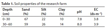
Data were collected from the first irrigation in each furrow. Inflow rates were determined by control valves connected to a concrete pipe at the upstream end of the field. Furrow cross-section parameters are based on the furrow geometry equation:

where A is the cross-sectional area, T is the top width, y is the furrow depth, and R is the hydraulic radius, presented in Table 2 as measured before the first irrigation.

 

 

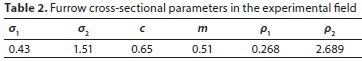
Infiltration parameters can be estimated by the observed advance data (Elliott et al., 1983; McClymont and Smith, 1996) or by a combination of advance and runoff data (Gillies and Smith, 2005; Scaloppi et al., 1995). The two-point method computes infiltration parameters with the measured advanced data (Gillies and Smith, 2005; Gillies et al., 2007; Guardo et al., 2000). Infiltration in the furrow was computed by the Lewis-Kostiakov equation Z = kτ^a + f₀τ, where Z is the water infiltrated volume per unit length of the furrow, τ is the intake opportunity time, f₀ is the final infiltration rate, and k and a are empirical parameters. The advance equation can be used to calculate infiltration parameters a and k in furrow irrigation as follows (Walker, 1989):

where x is the advance distance, t_adv is the advance time, and p and r are advance parameters. Walker and Skogerboe (1987) combined Lewis-Kostiakov, advance, and water balance equations and obtained the following equation:

where Q_in is the inflow rate; A₀ is the water cross-sectional area upstream of the furrow calculated from A₀ = (Q_inn/(ρ₁S^1/2))^1/ρ2 (Walker, 1989), n is the Manning coefficient, ρ₁ and ρ₂ are the furrow geometrical parameters, σ_y is the surface storage water profile shape factor assumed to be 0.75, and σ_z is the infiltrated water profile shape factor computed by the following equation (Walker, 1989):

where a is the exponent of the Lewis-Kostiakov equation and r is the advance curve parameter. Instead of using the two-point method, all the data from the stations have to be used to estimate k and a for each irrigation, since the slope and inflow rate are different throughout the furrow length. Therefore, Eq. 2 can be rewritten as follows (Sepaskhah and Shaabani, 2007):

The infiltration of the Lewis-Kostiakov equation can be calculated from Eq. 5. The values of V_x1 (the V_x parameter at 1 min interval) and a are estimated by regression analysis for V_x and t. Then, the k parameter is computed from K = V_x1/σ_z.

The infiltration parameters and properties of the experi-mental furrow for each irrigation event are shown in Table 3.

The application efficiency (E_a) for each experiment was computed by Eq. 6:

where V_in is the total volume of water applied at each irrigation; V_req is the water volume required in the soil profile; z_req is the soil moisture extracted by the crop between irrigations; L is furrow length; w is furrow spacing; t_co is cut-off time; and Q_o is inflow rate. The amount of water required in the root zone was assumed to be 50 mm for all experiments.

Runoff ratio was calculated from the following equation:

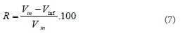
where V_inf is the infiltrated volume. Deep percolation (D_p) is the percentage of the infiltrated water that is unreachable for the plants and penetrates to the lower depths. D_p was obtained from Eq. 8.

 

RESULTS AND DISCUSSION

The advance and recession curves for both irrigation methods are presented in Figs 2 to 4. The advance times in the irrigation events S1, S2, S3, M1, M2, and M3 were 40.25, 23.16, 19.38, 63.36, 35.28, and 15.83 min, respectively. It can be observed that the advance time was significantly greater in MF than SF. In irrigation events M1 and M2, the advance time was, respectively, 57% and 52% larger than its counterpart in irrigation events S1 and S2. These results indicate that the flow velocity was lower in MF than in SF.

 

 

 

 

 

 

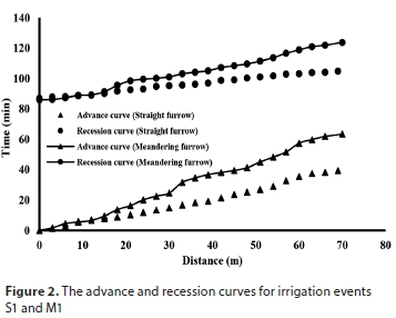
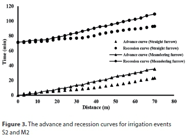
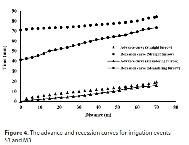
While the flow rate increased from 0.6 to 1.2 L∙s⁻¹, the advance time was reduced 42% and 44% for SF and MF irrigations, respectively. By varying the flow rate from 0.6 to 2.4 L∙s⁻¹ for SF irrigation and from 1.2 to 3.6 L∙s⁻¹ for MF irrigation, the advance time decreased 51% and 55%, respectively. The impact of changing the flow rate is almost the same for both irrigation methods, although the reduction of advance time is slightly greater in MF irrigation than SF irrigation.

The recession time was greater for MF than SF because of the higher water storage at the stations. During irrigation events M1 and M2, the recession time was 17% longer than its counterpart in irrigation events S1 and S2. The disappearance of water in the recession phase of MF irrigation is mostly because of the infiltration and not because of the outflow downstream of the furrow. The advance and recession curves were almost parallel for both furrow irrigation methods, which shows uniform infiltration throughout the furrows. As can be seen from Figs 2 and 3, advance times decrease when inflow rate increases and the difference in advance times between the two irrigation methods also decreases.

The values of inflow during irrigation events were 0.6, 1.2, 2.4, and 3.6 L∙s⁻¹. The runoff hydrographs of each irrigation event are presented in Figs 5-7. Runoff was notably less in MF than SF irrigation. As water flows in the MF, the direction of flow changes along the furrow, leading to an increase in the wetted perimeter and the infiltration depth. Furthermore, because of the lower velocity in MF irrigation, soil erosion is less compared to SF irrigation. The volumes of inflow and outflow during each irrigation event are shown in Table 3.

 

 

 

 

 

 

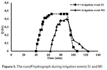
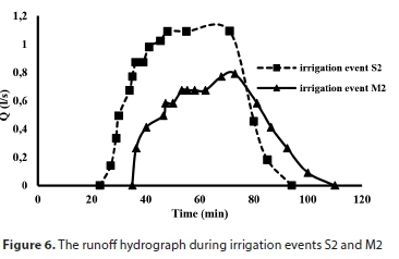
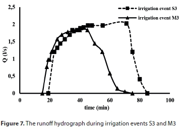
The flow rate and depth of water are affected by the basic infiltration rate (Sepaskhah and Afshar-Chamanabad, 2002), as confirmed by the findings of the present study (Table 3). According to Table 3, the basic infiltration rate for the same inflow is greater in MF than SF irrigation due to a higher wetted perimeter and flow depth. The parameters of the Kostiakov-Lewis equation for each experiment are presented in Table 3. In MF irrigation, the value of k is higher and the value of a is lower than in SF irrigation.

The values of k in MF irrigation with inflow rates of 0.6 and 1.2 L∙s⁻¹ are 18% and 67% higher than that for SF irrigation. By increasing the flow rate, the value of k is also increased in MF irrigation. The values of a decreased 18% and 46% for inflow rates of 0.6 and 1.2 L∙s⁻¹, respectively, in MF compared to SF irrigation. The runoff percentage, deep percolation, and application efficiency for each irrigation event are given in Table 4.

For MF irrigation (irrigation events M1 and M2), the runoff losses are 11.55-21.86 times lower than they are in SF irrigation (irrigation events S1 and S2). When the inflow rate was increased, the runoff also increased in SF irrigation. The deep percolation losses are significantly greater in MF than SF irrigation. MF irrigation can be recommended for plants with a deep root zone, heavy textured soil, and sloping fields.

The water application efficiency ranged from 25.66% (irrigation event S3) to 82.15% (irrigation event M1). In both methods, the lowest application efficiency values occurred with high inflow rates (irrigation events S3 and M3). In contrast, the highest application efficiency values occurred with low inflow rates. The application efficiency of MF irrigation is slightly greater than that of SF irrigation. According to Table 4, the difference in advance time between the two methods is not significant at the 5% level in S3 and M3 irrigation events. Despite the inflow rate in the M3 irrigation event being higher than in S3, the advance times are 95% similar. The table also shows that there is no difference in outflow volume between S1 and M3 irrigation events. The inflow rate in the M3 irrigation event is 6 times higher than for the S1 irrigation event and the outflow volumes are the same due to the fact that meandering furrow irrigation reduces the velocity of flow throughout the furrow and increases infiltrated water volume.

Batista et al. (2012) and Roldán-Cañas et al. (2013) reported that lower runoff losses and high application efficiency could be achieved by using low inflow rates. The values of the exponents and coefficients of the advance equations are presented in Table 5. These parameters are varied for straight and meandering furrows since the hydraulic condition is different in these furrows. These results also indicate that the flow velocity is lower in MF than SF.

 

 

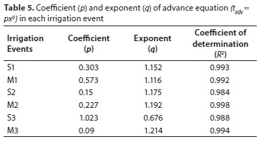
Irrigation events must be carefully implemented to achieve high efficiency. The MF system often requires a much greater labour input for construction and deep percolation in sandy soil is very high. Therefore, the type of soil and available labour are important factors in choosing the MF system. Harvesting requires a labour-intensive method in the MF system and harvest machines are not able to move easily in MF furrows. Therefore, further research is recommended into conducting, managing and harvesting with meandering furrow irrigation.

 

CONCLUSION

Field irrigation events were undertaken to evaluate the impact of MF and SF irrigation on performance and hydraulic and infiltration parameters. Advance and recession times were considerably greater in MF irrigation than SF irrigation. The average infiltrated water was lower in SF irrigation than MF irrigation. The recession times in MF irrigation were higher because of greater water storage in upstream stations. The parameters of the advance equation were estimated for MF and SF furrow irrigation and the results showed that the velocity of water advance was reduced in MF irrigation; therefore, runoff and erosion losses were also reduced. The disappearance of water in the recession phase would mostly be due to infiltration in MF irrigation and runoff in SF irrigation. The basic infiltration rate in the meandering furrow is higher than in the ordinary furrow. The coefficient of the infiltration equation, k, was higher and the exponent a was lower in the MF irrigation than in the SF irrigation. The application efficiency was better in the MF irrigation event with the inflow rate of 0.6 L∙s⁻¹ compared with other irrigation events. Therefore, selecting MF irrigation, reducing the inflow rate, and choosing an appropriate cut-off time can lead to improved irrigation efficiency. MF irrigation can be a viable alternative to expensive irrigation systems such as sprinkler or trickle irrigation.

 

REFERENCES

ALAZBA AA (1999) Simulating furrow irrigation with different inflow patterns. J. Irrig. Drain. Eng. 125 (1) 12-18. http://dx.doi.org/10.1061/(ASCE)0733-9437(1999)125:1(12)        [ Links ]

BARRIOS-MASIAS FH and JACKSON LE (2016) Increasing the effective use of water in processing tomatoes through alternate furrow irrigation without a yield decrease. Agric. Water Manage. 177 107-117. http://dx.doi.org/10.1016/j.agwat.2016.07.006        [ Links ]

BAUTISTA E, SCHLEGER JL and STRELKOFF TS (2012) WinSRFR 4.1, software and user manual. Arid Land Agricultural Research Center, Maricopa, AZ.         [ Links ]

ELLIOTT RL, WALKER WR and SKOGERBOE GV (1983) Infiltration parameters from furrow irrigation advance data. Trans. ASAE 26 (6) 1726-1731. http://dx.doi.org/10.13031/2013.33833        [ Links ]

GHARBI A, DAGHARI H and CHERIF K (1993) Effect of flow fluctuations on free draining, sloping furrow and border irrigation systems. Agric. Water Manage. 24 (4) 299-319. http://dx.doi.org/10.1016/0378-3774(93)90009-Y        [ Links ]

GILLIES MH, SMITH RJ and RAINE SR (2007) Accounting for temporal inflow variation in the inverse solution for infiltration in surface irrigation. Irrig. Sci. 25 (1) 87-97. http://dx.doi.org/10.1007/s00271-006-0037-9        [ Links ]

GILLIES MH and SMITH RJ (2005) Infiltration parameters from surface irrigation advance and run-off data. Irrig. Sci. 24 (1) 25-35. http://dx.doi.org/10.1007/s00271-005-0004-x        [ Links ]

GUARDO M, OAD R and PODMORE TH (2000) Comparison of zero-inertia and volume balance advance-infiltration models. J. Hydraul. Eng. 126 (6) 457-465. http://dx.doi.org/10.1061/(ASCE)0733-9429(2000)126:6(457)        [ Links ]

LEHRSCH GA, LENTZ RD, BJORNEBERG DL and SOJKA RE (2014) Erosion: Irrigation-induced. Reference module in Earth Systems and Environmental Sciences (Online database) 1-11. http://dx.doi.org/10.1016/B978-0-12-409548-9.09019-9        [ Links ]

LETEY J, HOFFMANB GJ, HOPMANSC JW, GRATTANC SR, SUAREZD D, CORWIND DL, OSTERA JD, WUA L and AMRHEINA C (2011) Evaluation of soil salinity leaching requirement guidelines. Agric. Water Manage. 98 502-506. http://dx.doi.org/10.1016/j.agwat.2010.08.009        [ Links ]

MCCLYMONT DJ and SMITH RJ (1996) Infiltration parameters from optimization on furrow irrigation advance data. Irrig. Sci. 17 (1) 15-22. http://dx.doi.org/10.1007/s002710050017        [ Links ]

MERGEN L (2014) The last station's water crisis. Energy New Comes Magazine 51 86-88 (in Persian).         [ Links ]

MINTESINOT B, VERPLANCKE H, VAN RANST E and MITIKU H (2004) Examining traditional irrigation methods, irrigation scheduling and alternate furrows irrigation on vertisols in northern Ethiopia. Agric. Water Manage. 64 (1) 17-27. http://dx.doi.org/10.1016/S0378-3774(03)00194-X        [ Links ]

MOSTAFAZADEH-FARD B, KAVEI-DEYLAMI R, SAGHAIAN-NEJAD SH and JALALIAN A (2010) The comparison of erosion of meandering and standard furrow irrigation under different field slopes. Aust. J. Agric. Eng. 1 (2) 29-37. http://dx.doi.org/10.1007/s10795-010-9093-7        [ Links ]

MOSTAFAZADEH-FARD B and MORAVEJALAHKAMI B (2006) The performance of Gholam-gardeshi furrow irrigation. Int. J. Agric. Biol. 8 (5) 698-702.         [ Links ]

REDDY JM, JUMABOEV K, MATYAKUBOY B and ESHMURATOV D (2013) Evaluation of furrow irrigation practices in Fergana valley of Uzbekistan. Agric. Water Manage. 117 133-144. http://dx.doi.org/10.1016/j.agwat.2012.11.004        [ Links ]

ROLDÁN-CAÑAS J, CHIPANA R, MORENO-PÉREZ M F and CHIPANA G (2015). Description and evaluation of zigzag furrow irrigation in the Inter-Andean Valleys of Bolivia. J. Irrig. Drain. Eng. 141 (11) 04015019(10). http://dx.doi.org/10.1061/(ASCE)IR.1943-4774.0000902        [ Links ]

ROLDÁN-CAÑAS J, MORENO-PÉREZ MF, GARCÍA MORENO FJ and CHIPANA R (2013) Application of WinSRFR4 program to zigzag corrugated furrow irrigation in Bolivia. Proc. 2013 European Geosciences Union (EGU) General Assembly. European Geosciences Union (EGU), Munich, Germany.         [ Links ]

SCALOPPI EJ, MERKLEY GP and WILLARDSON LS (1995). Intake parameters from advance and wetting phases of surface irrigation. J. Irrig Drain. Eng. 121 (1) 57-70. http://dx.doi.org/10.1061/(ASCE)0733-9437(1995)121:1(57)        [ Links ]

SEPASKHAH AR and AFSHAR-CHAMANABAD H (2002) Determin-ation of infiltration rate for every other furrow irrigation. Biosyst. Eng. 82 (4) 479-484. http://dx.doi.org/10.1006/bioe.2002.0088        [ Links ]

SEPASKHAH AR and SHAABANI MK (2007) Infiltration and hydraulic behavior of an anguiform furrow in heavy texture soils of Iran. Biosyst. Eng. 98 (2) 248-256. http://dx.doi.org/10.1016/j.biosystemseng.2007.03.024        [ Links ]

SIYAL AA, MASHORI AS, BRISTOW KL and VAN GENUCHTEN MTh (2016) Alternate furrow irrigation can improve water productivity of okra. Agric. Water Manage. 173 55-60. http://dx.doi.org/10.1016/j.agwat.2016.04.026        [ Links ]

SOROUSH F, MOSTAFAZADEH-FARD B, MOUSAVI SF and ABBASI F (2012) Solute distribution uniformity and fertilizer losses under meandering and standard furrow irrigation methods. Aust. J. Agric. Eng. 6 (5) 884-890.         [ Links ]

WALKER WR and SKOGERBOE GV (1987) Surface Irrigation: Theory and Practice. Prentice- Hall, Inc., Englewood Cliffs, New Jersey. 399 pp.         [ Links ]

WALKER WR (1989) Guidelines for designing and evaluating surface irrigation systems. FAO Irrigation and Drainage Paper No. 45. FAO, Rome.         [ Links ]

XIAO Y, ZHANG J, JIA TT, PANG XP and GUO ZHG (2015) Effects of alternate furrow irrigation on the biomass and quality of alfalfa. Agric. Water Manage. 161 147-154. http://dx.doi.org/10.1016/j.agwat.2015.07.018        [ Links ]

ZERHUN D, FEYEN J and REDDY JM (1996) Sensitivity analysis of furrow irrigation performance parameters. J. Irrig. Drain. Eng. 122 49-57. http://dx.doi.org/10.1061/(ASCE)0733-9437(1996)122:1(49)        [ Links ]

 

 

Received 8 June 2018
Accepted in revised form 23 September 2019

 

 

* Corresponding author, email: Rahimpour@uk.ac.ir

^rND^sALAZBA^nAA^rND^sBARRIOS-MASIAS^nFH^rND^sJACKSON^nLE^rND^sELLIOTT^nRL^rND^sWALKER^nWR^rND^sSKOGERBOE^nGV^rND^sGHARBI^nA^rND^sDAGHARI^nH^rND^sCHERIF^nK^rND^sGILLIES^nMH^rND^sSMITH^nRJ^rND^sRAINE^nSR^rND^sGILLIES^nMH^rND^sSMITH^nRJ^rND^sGUARDO^nM^rND^sOAD^nR^rND^sPODMORE^nTH^rND^sLETEY^nJ^rND^sHOFFMANB^nGJ^rND^sHOPMANSC^nJW^rND^sGRATTANC^nSR^rND^sSUAREZD^nD^rND^sCORWIND^nDL^rND^sOSTERA^nJD^rND^sWUA^nL^rND^sAMRHEINA^nC^rND^sMCCLYMONT^nDJ^rND^sSMITH^nRJ^rND^sMERGEN^nL^rND^sMINTESINOT^nB^rND^sVERPLANCKE^nH^rND^sVAN RANST^nE^rND^sMITIKU^nH^rND^sMOSTAFAZADEH-FARD^nB^rND^sKAVEI-DEYLAMI^nR^rND^sSAGHAIAN-NEJAD^nSH^rND^sJALALIAN^nA^rND^sMOSTAFAZADEH-FARD^nB^rND^sMORAVEJALAHKAMI^nB^rND^sREDDY^nJM^rND^sJUMABOEV^nK^rND^sMATYAKUBOY^nB^rND^sESHMURATOV^nD^rND^sROLDÁN-CAÑAS^nJ^rND^sCHIPANA^nR^rND^sMORENO-PÉREZ M^nF^rND^sCHIPANA^nG^rND^sSCALOPPI^nEJ^rND^sMERKLEY^nGP^rND^sWILLARDSON^nLS^rND^sSEPASKHAH^nAR^rND^sAFSHAR-CHAMANABAD^nH^rND^sSEPASKHAH^nAR^rND^sSHAABANI^nMK^rND^sSIYAL^nAA^rND^sMASHORI^nAS^rND^sBRISTOW^nKL^rND^sVAN GENUCHTEN^nMTh^rND^sSOROUSH^nF^rND^sMOSTAFAZADEH-FARD^nB^rND^sMOUSAVI^nSF^rND^sABBASI^nF^rND^sXIAO^nY^rND^sZHANG^nJ^rND^sJIA^nTT^rND^sPANG^nXP^rND^sGUO^nZHG^rND^sZERHUN^nD^rND^sFEYEN^nJ^rND^sREDDY^nJM^rND^1A01^nCB^sMac Bean^rND^1A01^nAA^sIlemobade^rND^1A01^nCB^sMac Bean^rND^1A01^nAA^sIlemobade^rND^1A01^nCB^sMac Bean^rND^1A01^nAA^sIlemobade

RESEARCH PAPERS

 

An evaluation of the primary South African standard and guideline for the provision of water for firefighting

 

 

CB Mac Bean; AA Ilemobade^*

School of Civil and Environmental Engineering, University of the Witwatersrand, Johannesburg, Private Bag 3, WITS 2050, South Africa

 

 

---

ABSTRACT

In South Africa, as is mostly the norm globally, national legislation and guidelines specify that potable water distribution networks maintain the capacity to provide specified quantities of water for firefighting. This paper addresses the question: is the South African standard and guideline pertaining to fire-flow provision appropriate for firefighting and do these ensure the most efficient balance between providing sufficient fire protection and promoting sustainable water use? In answering this question, this study: (i) reviewed national and international design standards and guidelines; and (ii) captured and analysed 10 years of billable fire incident reports representing 3 859 fire events within the City of Johannesburg. Highlights from the study include: inconsistencies in categories when comparing the SANS 10090 and The Red Book fire tables and violations (in The Red Book) of stipulated Minimum Fire Flows; over the 10 year period, 75% of fire incidents within the City of Johannesburg were extinguished using less than 6.6 kL of water - less than the capacity (6.9 kL) of the City's conventional pumping tanker during the period; 99.9% of fire incidents within the City were quenched using an average fire flow rate of less than 1 200 L/min, which is the minimum hydrant flow rate for the lowest fire risk category in SANS 10090; and peak fire occurrence did not correspond with typical peak residential water use. Recommendations are proffered in respect of the above.

Keywords: firefighting water standard and guideline

---

 

 

INTRODUCTION

Water conservation has become a priority for many water-scarce countries around the world, including South Africa. With the majority of potable water supply to the public being delivered via municipal water systems, it is critical that these systems be designed, constructed and maintained in such a manner that they promote the most efficient use of water. Inseparable from the topic of efficient potable water use, is the efficient or inefficient provision of potable water for firefighting and the impact that this provision has on water distribution systems (WDSs) and water conservation.

A global consensus on the ideal design philosophy for providing water for firefighting remains to be established. Likewise, civil infrastructure standards linked to firefighting remain diverse and widely debated, as engineers face the challenge of balancing firefighting water provision against efficient water use. It is due to this complex trade-off between ensuring adequate supply of water for firefighting and minimizing water use that further research into this topic is critically needed.

In South Africa, the national standard (SANS 10090; SABS, 2003) and guideline (DHS and CSIR, 2019) recommend that potable water distribution mains have and maintain the capacity, both in flow (L/min) and pressure head (m), to provide specified quantities of water for firefighting purposes. As a result, a dominant design constraint on WDSs is providing for fire flow, which is defined as the rate of flow of water required by the firefighting service for the extinguishing of fires (SABS, 2003).

Since fire flows significantly influence the sizing of a reticulated network, it is important that these requirements are defined as accurately as possible. It is interesting to note that the demand for water supplies during firefighting is believed, by some, to be historically based on instinct and was strongly characterised by what was available rather than a technical analysis of what was needed (Law and Beever, 1995; Davis, 2000).

The condition of infrastructure, development of firefighting technologies and techniques, and the growth in fire safety awareness have all progressed with time and evolved dramatically since 1966 when the national codes for the provision of water for firefighting in South Africa were first published. Therefore, Van Zyl and Haarhoff (1997) recommend that the provision and requirements for fire flows be amended to reflect present conditions and technologies.

Objectives

This study addresses two objectives:

•To present an analysis of international and South African design standards and guidelines pertaining to water provision for firefighting

•To present actual fire flow data recorded in the City of Johannesburg, to compare this data with the primary South African standard and guideline values, and to make recommendations to guide future revisions of the primary South African design standard and guideline for the provision of water for firefighting

South African standards and guidelines for fire flows

Guidelines are intended to assist decision-making, whereas standards are enforceable absolute limits (Schlotfeldt, 1995 cited in CSIR, 2005). The national standard (also termed 'code') for the provision of water for firefighting in South Africa titled 'Community protection against fire' was first published in 1966 (SABS 090) and revised in 1972 (SABS, 1972). This code was compiled with the assistance of organizations from the UK, USA, Canada, New Zealand and Germany (Van Zyl and Haarhoff, 1997). A notable feature of this code is the absence of minimum water pressures for both water provision and the pumping ability of response units during a firefighting event. A summary of fire flow values within the most recent edition of this standard (i.e. SANS 10090: SABS, 2003) is shown in Table 1.

A separate national code, SANS 10252-1:2016 (SABS, 2016) titled 'Water supply and drainage for buildings Part 1: Water supply installations for buildings' addresses design pressures and flows for fire installations. A minimum provision of 30 L/min per fire hose reel and 1 200 L/min per hydrant is stipulated without any reference to fire risk categories. This code neither refers to SANS 10090 nor provides as much detail as it does. However, SANS 10252-1 stipulates that a minimum pressure of 300 kPa must be maintained in hoses and hydrants.

Another industry-recognised reference that provides guidance on firefighting is the recently released Red Book (DHS and CSIR, 2019) titled The Neighbourhood Planning and Design Guide (Red Book): Creating Sustainable Human Settlement. The Red Book (DHS and CSIR, 2019) is an updated version of the CSIR (2005) Guidelines for Human Settlement Planning and Design. In contrast to the CSIR (2005) firefighting guidelines, The Red Book (DHS and CSIR, 2019) references the SABS 10090 (2003) code. The Red Book's fire flow values are presented in Table 2.

A notable distinction between SANS 10090 (SABS, 2003) and The Red Book (DHS and CSIR, 2019), apart from the different values they stipulate, is their differing fire risk categories. The Red Book presents a single set of fire risk categories to which all its various recommendations are related. SANS 10090, however, presents two categories. The first is titled, 'Fire Risk Category', and the second, which is a subset of the first, is titled, 'Possible Fire Sizes'. The 'Possible Fire Sizes' category is used exclusively to determine 'Minimum Fire Flow' rates. An adverse consequence of having two categories in the SANS 10090 is that the Minimum Fire Flow and the Minimum Hydrant Flow are determined from different Fire Risk Categories, despite the fact that both are within the same table and connected. By way of example, an affluent residential area (Category C) where houses are spaced further than 30 m apart (Category D1) would have SANS 10090 recommend two Minimum Hydrant Flows of 2 000 L/min (Category C) and 1 200 L/min (Category D1) and two Minimum Fire Flows of 6 000 L/min (Category C) and 1 900 L/min (Category D1).

In addition to the above matter, some violations arise when employing Minimum Fire Flow values from The Red Book. The Red Book, which is a guideline that is intended to assist decision-making, should not, without reasonable justification, violate standards (in this instance, SANS 10090), which present enforceable absolute minimum limits (Schlotfeldt, 1995 cited in CSIR, 2005). All fire flow values in The Red Book are less than the values stipulated in SANS 10090 for similar fire risk categories. An example of this violation is seen in the first two fire risk categories in both documents - The Red Book recommends a fire flow of 6 ٠٠٠ L/min for the 'high risk' category and 3 ٠٠٠ L/min for the 'moderate risk 1' category; SANS 10090, on the other hand, stipulates 13 000 L/min and 9 000 L/min, respectively, for Categories A and B. This paper recommends a uniform category for both documents and Minimum Fire Flows that are consistent with analysed data.

International standards and guidelines for fire flows

Across the world, many methods have been developed to calculate fire flows. These methods generally form the basis on which fire protection codes, such as those discussed above, are established. These methods regulate the design of various WDS features such as:

•Spacing of fire hydrants

•Minimum size of reticulation pipes

•Minimum flow rates and pressures

•Storage requirements and flow durations

In a report conducted by The Fire Protection Research Foundation, titled 'Evaluation of fire flow methodologies', 16 fire flow calculation methods were evaluated. The methods identified were from the USA, UK, France, Germany, the Netherlands, New Zealand, and Canada. Eleven of the methods address pre-incident infrastructure/building planning (see (a) below) and five are best suited for on-scene firefighting (see (b) below) (Benfer and Scheffey, 2014):

(a) Infrastructure/building planning: These methods are necessarily predictive in nature, are more complicated and involve several steps and multiple calculations. Typical variables accounted for include: building construction, occupancy, fire size, heat release and sprinkler contribution. The inclusion of a variety of variables enables adjustments to be made to the building type or protection features (e.g. adding a sprinkler system) in order to reduce the fire flow.

(b) On-scene firefighting: These methods, by comparison, are much simpler, allowing fire fighters on the scene to assess whether they need more hose lines or apparatus to fight the fire. They typically consist of one equation with one independent variable - either the volume or area of the fire.

The 16 fire flow calculation methods were simulated for two differently sized non-residential buildings and two differently sized single-family residential buildings. Their study included both sprinklered and non-sprinklered calculations. Figure 1 shows the fire flow requirements for a non-sprinklered, non-residential building of 50 000 ft² (4 645 m²).

To compare the primary South African fire flow standard (SANS 10090:2003, SABS, 2003) and guideline (The Red Book, 2019) with the 16 shown on Fig. 1, the Minimum Fire Flow requirements for a simlar structure, as defined in SANS 10090 and The Red Book, are superimposed on the results presented in the figure. It is important to note that the SANS 10090 fire flow values presented in Figs 1 and 2 do not explicitly deal with a single incident. However, as expressed in SANS 10090 (SABS, 2003) clause 11.4.1: 'The required fire flow should be available to the firefighting team on arrival at the fire.' It is thus assumed that the comparison made below is fair. Where applicable, both the Minimum Fire Flow and Minimum Hydrant Flow for SANS 10090 and The Red Book are shown in Figs 1 and 2.

Employing the SANS 10090 (2003) 'Possible Fire Sizes' category 'Non-residential buildings with divisions not greater than 5 000 m² (53 800 ft²)', a Minimum Fire Flow of 13 000 L/min is required (Fig. 1). In the figure, the SANS 10090 requirement falls within the ranges of the ISO, IFC/NFPA 1, and the IWUIC Building Planning methods but is, for several of the other methods, several orders of magnitude lower. The Minimum Fire Flow requirement in The Red Book for the 'high risk' category (which is a similar category to the SANS 10090 category above) is 6 ٠٠٠ L/min. The corresponding Minimum Hydrant Flow for SANS 10090 and The Red Book are ٢ ٠٠٠ L/min and 1 500 L/min, respectively.

It is seen from Fig. 1 that the range of possible fire flows is large, not only when comparing the various methods, but also within some ranges. The FEDG and PAS 4509 methods have the largest ranges. Furthermore, as can be seen in Fig. 1, the Building Planning methods tend to recommend fire flows that are higher than the on-scene methods. many of the on-scene firefighting methods do not incorporate sprinkler protection systems in their calculations (Benfer and Scheffey, 2014).

Figure 2 shows the sprinklered and non-sprinklered fire flow values for a residential building of 3 500 ft² (325 m²).

Employing the SANS 10090 Risk Category D1 - 'Houses > 30 m apart', a Minimum Fire Flow of 1 900 L/min and a Minimum Hydrant Flow of ١ ٢٠٠ L/min are required. Employing The Red Book 'low risk' category, the Fire Flow and the Minimum Hydrant Flow are each 900 L/min.

For residential buildings fitted with sprinklers, it is worth noting that 12 out of the 18 Benfer and Scheffey (2014) methodologies shown on Fig. 2 required the same fire flow as non-sprinkler fitted buildings. However, as seen in Fig 1 and 2, Minimum Fire Flow requirements vary greatly across many countries.

 

METHODS

Fire incident reports within the City of Johannesburg

A fire incident report (or call slip) is a physical document that is filled out and submitted to the central Emergency Management Services (EMS) headquarters after each fire incident attended to by the fire brigade. Only billable (i.e. incidents that the fire department charges the property owner for services rendered) fire incident reports are digitally captured in spreadsheets by the EMS. Billable fire incident reports are best explained by sections 10.1 and 10.2 (Fees) of the Fire Brigade Services Act No. 99 (RSA, 1987). These sections (listed below) outline the basis on which the local fire department may charge for services rendered:

(1) A controlling authority may, subject to any condition contemplated in section 11(2)(a), determine the fees payable by a person on whose behalf the service of the controlling authority is applied-

(a) for the attendance of the service;

(b) for the use of the service and equipment; or

(c) for any material consumed.

(2) A person on whose behalf, in the opinion of the chief fire officer concerned, a service of a controlling authority has been employed, may in writing be assessed by that chief fire officer for the payment of the fees referred to in subsection (1) or any portion thereof.

It is the above billable incidents that have been consolidated and presented in this paper. In these reports, details captured include the duration of the call out, the quantity of water used, and the appliances used during the incident (see an example in Table 3). On-site calculations are carried out to estimate the total fire flow volume released during the incident. These calculations account for water obtained from fire trucks, water tankers, and hydrants.

The volume or flow rate is determined by reading the meters installed on each appliance. In this paper, the fire incident reports discussed are for fire incidents within the City of Johannesburg only and for the past 10 years (1 January 2006 to 30 September 2017).

Table 3 shows an example fire incident report which was used for invoicing purposes. In the table, it can be seen that 4 different stations responded to one emergency and a total of 30 kL of water was used for firefighting. The Malvern unit was on-site for the longest duration - 2 h 27 min. It is assumed that fire flow rate extracted from the municipal network was constant over the on-site firefighting duration. While this assumption produces an average flow rate per incident (Eq. 1), it underestimates the peak firefighting flow (data which were not, and currently are not, recorded).

From 1 January 2006 to 30 September 2017, there were 4 556 billable firefighting incident reports recorded in the City of Johannesburg. Of this number, 697 were recorded as incidents that did not require municipal water and, therefore, the analysis below was based on 3 859 billable water use incidents. This dataset excludes all non-billable fire incidents including informal settlements, veld/grass and car/motorcycle fires.

 

RESULTS AND DISCUSSION

The scatter plot shown in Fig. 3 shows the magnitude and distribution of the 3 859 fire flow volumes recorded from 1 January 2006 to 30 September 2017. Figure 4 shows the magnitude and distribution of the 3 859 fire flow rates from 1 January 2006 to 30 September 2017. To gauge the validity of the incidents with large fire flow volumes (> 300 kL) and fire flow rates (> 1 000 L/min), fire event characteristics (such as duration, number of responding stations, presence of fire safety officials, and fire location) were individually examined. From this exercise, the fire incident circled in Figs 3 and 4 was identified as a likely data capture error because it did not bear the same characteristics as the other large fire volume incidents. The largest (800 kL) fire flow volume in the dataset was responded to by 6 different fire stations, lasted over 15 h and had fire safety officials present.

 

 

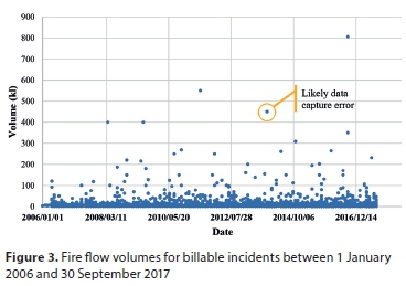
Figure 4 also includes the SANS 10090 (2003) standard and The Red Book (DHS and CSIR, 2019) guideline values for Fire Flow as well as the Minimum Hydrant Flow for the different fire risk categories. An assumption made in the below analysis is that the recorded firefighting flows extracted from the municipal network or fire equipment were what was required to fight the fires. None of the 3 859 billable fire incident reports indicate otherwise.

Figure 4 reveals that over the 10-year period, not a single fire incident in the City of Johannesburg recorded an average flow rate greater than 6 000 L/min. This implies that over the 10-year period, no incident can be classified as a SANS 10090 Category A, B or C nor The Red Book 'high risk' category fire. During the 10-year period, only 2 incidents recorded average flow rates greater than 2 000 L/min. Three incidents recorded average flow rates greater than 1 500 L/min. The vast majority of average flow rates fell below both the SANS 10090 Minimum Hydrant Flow for Categories A, B, C and D and The Red Book Minimum Hydrant Flow for 'high risk' and 'moderate risk' categories.

Figure 5 shows that 75% of fire incidents were extinguished using less than 6.6 kL of water -this volume is less than the capacity (6.9 kL) of a conventional pumping tanker within the City of Johannesburg's fleet purchased in 2003. This means that over the study's 10-year period, 75% of fire incidents in the City of Johannesburg could have been extinguished without the use of municipal fire hydrants if a pumping tanker with a full tank of water was dispatched. The below quote from Myburgh and Jacobs (2014 p.11) confirms similar results obtained for 3 municipal areas in the Western Cape: 'only 8.6% of all fires were extinguished using water from the WDS by connecting firefighting equipment to a fire hydrant at the time of the fire. Most fires were extinguished by means of water ejected from a pre-filled tanker vehicle disconnected from the WDS at the time of fighting the fire.'

 

 

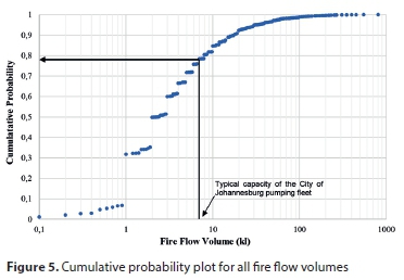
Figure 6 presents the cumulative probability plot of average flow rates, with the SANS 10090 and The Red Book values superimposed. The figure shows that 99.9% of all fire incidents within the City during the designated period resulted in an average fire flow rate less than 1 200 L/min, which equals the lowest of the Minimum Hydrant Flow rates for SANS 10090 (i.e. Category D). Likewise, 99.7% of all fire incidents resulted in an average fire flow rate less than 900 L/min, which equals the Minimuim Hydrant Flow rate for The Red Book's lowest fire risk category (i.e. low risk). These findings suggest that there is scope to reduce the current Minimum Fire Flows especially in low risk categories whilst maintaining adequate levels of safety. Because of the need to fight low probability but high consequence fires in moderate- to high-risk fire category areas, the authors caution on the application of the above statement to these areas.

To better understand intra-day and intra-year firefighting trends, Fig. 7 shows, over an average month, the average volume of water used to extinguish fires in relation to the frequency of fire occurrence while Fig. 8 shows the frequency of occurrence of fires and residential water use over a typical day. In Fig. 7, the green bar chart shows the average number of fire incidents occurring each month while the blue bar chart shows the average fire flow volume per incident for each month over the period 1 January 2006 to 30 September 2017. An expected seasonal trend is observed with regard to frequency of fire occurrence, with a notable rise in incidents from June to October, which are typically dry and low-rainfall months in Johannesburg. While average fire flow volumes range between 7 to 12 kL per incident, there is no observable seasonal trend. These trends imply that, while the frequency of fire occurrence is strongly related to climatic conditions, the volume of water used to quench fires, and by implication, the size of the fires, is not a function of climatic conditions within the City of Johannesburg. As a consequence, seasonal peak factors for fire flows may not be necessary when incorporating the provision for water for firefighting in the design of municipal mains within the City of Johannesburg or other metropolitan municipalities with similar fire flow and climatic conditions.

 

 

 

 

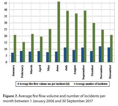
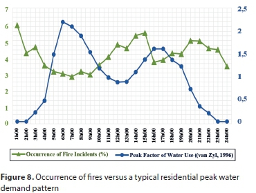
Figure 8 displays the occurrence of incidents throughout the course of a day, averaged over the period 1 January 2006 to 30 September 2017. The green graph shows the percentage distribution of fire incident start times. In Fig. 8, three peaks (at 01:00, 15:00 and 20:00) are observed. The highest of the three was at 01:00 - this represents 230 (5.9%) fire incidents. The blue graph shows a typical diurnal residential water use pattern published by Van Zyl (1996) (cited in Scheepers, 2012). The water use pattern shows the primary peak residential demand occurring at 06:00 while the secondary peak demand occurs between 16:00 and 17:00. When compared to the start times of fires within the City of Johannesburg, it is observed that the start times of peak fires do not correspond with peak residential water demand periods. The inverse is the case - the lowest observed start times of fires were during peak demand periods. This finding may therefore provide motivation to further investigate the recommendation to cater for both instantaneous peak demand and fire demand during WDS design as recommended by The Red Book (DHS and CSIR, 2019: J.3.2.2) i.e.: 'Conveyance infrastructure should have sufficient capacity for peak demand conditions and fire-flow requirements, in accordance with the design guidelines in this document' and (CSIR, 2005: volume 2, Chapter 9, page 27): 'The nominal capacity of the duty pump should be equivalent to the sum of the instantaneous peak demand and the fire demand (obtained from the section on provision of water for firefighting), or the instantaneous peak demand plus an allowance of 20%, whichever is the greater.'

 

CONCLUSIONS AND RECOMMENDATIONS

The key results and recommendations arising from the two objectives addressed in this study are presented below:

•Objective 1: To present an analysis of international and South African design standards and guidelines pertaining to water provision for firefighting

o A review of national and international standards and guidelines for water provision for firefighting are presented in the text. A notable distinction between the SANS 10090 (SABS, 2003) standard and The Red Book (DHS and CSIR, 2019) guideline, apart from the different values they recommend for Fire Flow and Minimum Hydrant Flow, is their differing fire risk categories. The Red Book presents a single set of fire risk categories while SANS 10090 presents two fire risk categories which, in certain instances, do not recommend consistent fire flow values for the same category.

o In addition, The Red Book, which is a guideline, in all instances, violates the Minimum Fire Flows in SANS 10090, which is a standard that stipulates minimum acceptable values.

o It is therefore a recommendation of this paper that the SANS 10090 fire risk categories (A, B, C, D and E) be revised. As a result of their simplicity and recent revision, The Red Book (DHS and CSIR, 2019) fire risk categories may be adopted in the recommended revision of the SANS 10090 fire risk categories.

•Objective 2: To present actual fire flow data recorded in the City of Johannesburg, to compare this data with the primary South African standard and guideline values, and to make recommendations to guide future revisions to the primary South African design standard and guideline for the provision of water for firefighting.

o Fire incident reports were obtained from the City of Johannesburg's EMS for the period 1 January 2006 to 30 September 2017. These reports show that the majority of average fire flow rates fell below both the SANS 10090 (2003) and The Red Book (DHS and CSIR, 2019) Minimum Hydrant Flow for all its categories. The below highlights are evidence of this:

◉ Almost all (99.9%) fire incidents recorded an average fire flow rate less than 1 200 L/min - the lowest Minimum Hydrant Flow rate for the SANS 10090 Categories

◉ Similarly, 99.7% of all fire incidents recorded an average extracted fire flow rate less than 900 L/min - the lowest Minimuim Hydrant Flow rate for The Red Book's categories

o A second finding from the analysis of fire incident reports was that 75% of fire incidents were extinguished using less than 6.6 kL of water and thus could have been extinguished using one of the City of Johannesburg's conventional pumping tankers which have a capacity of 6.9 kL. This, by implication, means that 75% of fire incidents within the City could have been extinguished without the use of municipal fire hydrants if a suitable tanker with a full tank of water was available.

o A third highlight was that, while the frequency of fire occurrence was strongly related to climatic conditions, the volume of water used to quench the fires was not a function of climatic conditions

o A fourth highlight was that the start times of peak fires did not correspond with peak residential water use periods within the City of Johannesburg over the 10-year period. The inverse was however the case - the lowest observed fire incidents occurred during peak demand periods

Based on the above findings, and the assumption that the results from this study can be generically applied, the following recommendations can be made:

•A Minimum Hydrant Flow of 1 200 L/min is recommended for all SANS 10090 and The Red Book Categories. SANS 10252-1:2012 (SABS, 2012) stipulates the same value.

•To improve the efficiency of firefighting within the City of Johannesburg, especially considering the potential devastation that could occur due to increasing instances of water cuts and low pressures (Kahanji et al., 2019), EMS should focus on acquiring pumping appliances with sufficient capacity and volume (minimum of 6.6 kL) to extinguish fires.

Based on the findings of this study, future research may investigate:

•The need for seasonal peak factors when incorporating the provision for water for firefighting in the design of municipal mains

•Catering for both instantaneous peak demand and fire demand during WDS design as recommended by The Red Book (DHS and CSIR, 2019)

•Understanding the change in rate of water use during a fire event

 

ACKNOWLEDGEMENTS

The participation and data provided by the City of Johannesburg's Emergency Management Services personnel are gratefully acknowledged. Also gratefully acknowledged is the postgraduate funding and support by Mott MacDonald.

 

REFERENCES

BENFER M and SCHEFFEY J (2014) Evaluation of Fire Flow Methodologies. The Fire Protection Research Foundation, Quincy, Massachusetts. https://doi.org/10.1007/978-1-4939-2889-7        [ Links ]

CSIR (2005) Guidelines for Human Settlement Planning and Design. Red Book. CSIR Building and Construction Technology, Pretoria.         [ Links ]

DHS and CSIR (Department of Human Settlements, South Africa and Centre for Scientific and Industrial Research (2019) The Neighbourhood Planning and Design Guide (Red Book): Creating Sustainable Human Settlement. DHS and CSIR, Pretoria. ISBN 978-0-6399283-2-6.         [ Links ]

DAVIS SK (2000) A review of fire fighting water requirements. ME thesis, University of Canterbury.         [ Links ]

KAHANJI C, WALLS RS and CICIONE A (2019) Fire spread analysis for the 2017 Imizamo Yethu informal settlement conflagration in South Africa. Int. J. Disaster Risk Reduct. https://doi.org/10.1016/j.ijdrr.2019.101146        [ Links ]

LAW M and BEEVER P (1995) Magic numbers and golden rules. Fire Saf. Sci. 4 79-84. https://doi.org/10.3801/IAFSS.FSS.4-79        [ Links ]

MYBURGH HM and JACOBS HE (2014), Water for firefighting in five South African towns. Water SA 40 (1) 11-17. http://dx.doi.org/10.4314/wsa.v40i1.2        [ Links ]

RSA (Republic of South Africa) (1987) Fire Brigade Services Act. Act No. 99 of 1987. Government Gazette 11006, 23 October 1987, Issue 99.         [ Links ]

SABS (South African Bureau of Standards) (1972) SABS 090:1972. Community protection against fire. SABS, Pretoria.         [ Links ]

SABS (South African Bureau of Standards) (2003) SANS 10090:2003 South African National Standard. Community protection against fire. Standards South Africa (a division of SABS), Pretoria. ISBN 0-626-14666-6        [ Links ]

SABS (South African Bureau of Standards) (2012) SANS 10252-1:2012. South African National Standard. Water supply and drainage for buildings Part 1: Water supply installations for buildings. SABS Standards Division, Pretoria.         [ Links ]

SCHEEPERS HM (2012) Deriving peak factors for residential indoor water demand by means of a probability based end-use model. Master of Science in Engineering, Stellenbosch University.         [ Links ]

SCHLOTFELDT CJ (1995) The "Red Book": Background, purpose and way forward. Paper presented at Red Book Workshops. February and March, Bloemfontein, Cape Town, Pretoria, Durban and Port Elizabeth.         [ Links ]

VAN ZYL JE (1996) Peak factors in municipal water reticulation networks. Proceedings of the Water Institution of South Africa Biennial Conference and Exhibition, 20-23 May 1996, Port Elizabeth, South Africa.         [ Links ]

VAN ZYL JE and HAARHOFF J (1997) South African fire water guidelines and their impact on water supply system cost. J. S. Afr. Inst. Civ. Eng. 39 (1) 16-22.         [ Links ]

 

 

Received 23 August 2018
Accepted in revised form 26 September 2019

 

 

* Corresponding author, email: adesola.ilemobade@wits.ac.za

^rND^sLAW^nM^rND^sBEEVER^nP^rND^sMYBURGH^nHM^rND^sJACOBS^nHE^rND^sVAN ZYL^nJE^rND^sHAARHOFF^nJ^rND^1A01^nT^sGoga^rND^1A01^nE^sFriedrich^rND^1A02^nCA^sBuckley^rND^1A01^nT^sGoga^rND^1A01^nE^sFriedrich^rND^1A02^nCA^sBuckley^rND^1A01^nT^sGoga^rND^1A01^nE^sFriedrich^rND^1A02^nCA^sBuckley

RESEARCH PAPERS

 

Environmental life cycle assessment for potable water production - a case study of seawater desalination and mine-water reclamation in South Africa

 

 

T Goga^I; E Friedrich^{I, *}; CA Buckley^II

^ICivil Engineering Programme, School of Engineering, University of KwaZulu-Natal, Durban, 4041, South Africa
^IIPollution Research Group, Chemical Engineering Programme, School of Engineering, University of KwaZulu-Natal, Durban, 4041, South Africa

 

 

---

ABSTRACT

Water is becoming a scarce resource in many parts of South Africa and, therefore, numerous plans are being put in place to satisfy the increased urban demand for this resource. Two of the methods currently considered are desalination of seawater and reuse of mine-affected water based on the use of reverse osmosis (RO) membranes. Due to their high energy consumption and associated environmental impacts, these methods have been under scrutinity and, therefore, an LCA was undertaken for both methods. To allow comparison between the two, the functional unit of 1 kL of potable water was specified. Design data were collected for both the construction and operation phases of the plants while SimaPro was used as the LCA analysis software with the application of the ReCiPe Midpoint method. The results indicate that the operation phase carried a greater environmental burden than the materials required for the infrastructure. In particular, electricity production and consumption is responsible for the majority of environmental impacts that stem from the respective plants. The total energy consumption of the proposed desalination plant is 3.69 kWh/kL and 2.16 kWh/kL for the mine-water reclamation plant. This results in 4.17 kg CO₂ eq/kL being emitted for the desalination plant and 2.44 kg CO₂ eq/kL for the mine-affected plant. A further analysis indicated that replacing South African electricity with photovoltaic (solar) and wind power has the potential to bring significant environmental benefits. The integration of these renewable energy systems with desalination and membrane treatment of mine-affected water has been proven to reduce environmental burdens to levels associated with conventional water technologies powered by the current electricity mix.

Keywords: LCA, water treatment, mine water, desalination

---

 

 

INTRODUCTION

Water is regarded as one of the most precious and critical resources worldwide. In South Africa, the scarcity of water presents various challenges, mainly relating to efficient development, management and utilisation (Knüppe, 2011). To overcome these obstacles and ensure that South Africa has sufficient water supply, various water treatment techniques have been explored. As is the case with all industrial processes, there are substantial environmental impacts that occur from the construction of the infrastructure, through to commissioning, operation and decommissioning. In order to effectively evaluate the environmental burden of each water treatment system as well as its associated processes, a life cycle assessment (LCA) can be utilised. The use of such a sustainability tool provides a true reflection of the product's life cycle from 'cradle to grave' by systematically quantifying the amount of energy used, the consumption of raw materials, emissions to the atmosphere as well as the amount of waste generated (ISO, 2006).

The use of LCA as an assessment tool to gauge the environmental impacts of water technologies has been increasingly used since the late 1990s. Loubet et al. (2014) and Buckley et al. (2011) present a comprehensive review of the applications of environmental LCAs in the water industry both internationally and locally. Assessments have been successfully conducted locally for conventional technologies utilised in potable water and wastewater treatment plants (Friedrich et al., 2007); however, there are only two local studies researching membrane processes. Internationally, such membrane processes have been the focus of many LCAs, with Meijers et al. (1998) starting this trend. Zhou et al. (2014) present an extensive review of the international studies employing LCAs for desalination and they include more than 30 individual research papers. Locally, there are only two such investigations (Friedrich, 2002; Ras and Von Blottnitz, 2012) that employ LCA for the use of membranes in the treatment of water. However, there are no such investigations for the local desalination of seawater or reclamation of mine-affected water. Therefore, this paper aims to satisfy this need by investigating the environmental burdens associated with membrane-based treatment processes.

This study compared two water treatment processes in South Africa to produce potable water. The first study is based on a proposed desalination plant that will be installed by Umgeni Water. During the feasibility study phase, it was determined that the plant should be located on the South Coast of KwaZulu-Natal and will be designed to produce a total of 150 ML/d of potable water (Umgeni Water, 2015a). The second study revolves around a water treatment process in Mpumalanga that treats mine-affected water to potable water standards. The plant is currently treating 15 ML/d of raw water via two processing trains (Golder Associates Africa, 2012). Both plants make use of membrane technologies to achieve the desired separation. Currently, these alternative sources of water and associated technologies are in rare use (DWA, 2013). However, considering the increasing demand for a limited resource, such operations will become more widespread. Thus, it is imperative to shape the design process for future projects from the outset, so as to reach the best outcome locally. The findings from this study will provide guidance regarding focus areas to guide this process.

The LCA process consists of 4 phases, namely, goal and scope definition, inventory analysis, impact assessment and interpretation (ISO, 2006). The first stage set the aims of the study and provided an outline of the functional unit, assumptions made and data requirements. The next stage consisted of the gathering of data which was used as inputs into SimaPro which was the selected LCA software. A series of scores for the various environmental impacts were obtained which provided an indication of the environmental contribution of the process parameters. Recommendations based on these results were then proposed.

 

CASE STUDIES

The first case study centred around a proposed desalination plant in the Southern eThekwini area that makes use of RO technology. The second case study focused on a mine-water reclamation process in Mpumalanga that was designed using both UF and RO.

Desalination plant in eThekwini Municipality

To determine the feasibility of constructing a large-scale desalination plant, an investigation by Umgeni Water was initiated by undertaking a desalination pre-feasibility study. After much consultation, a revised strategy was adopted where the detailed feasibility study would consider the option of a 150 ML/d plant situated on both the North and South Coast (Meier, 2012). A diagram of the desalination process highlighting the key components is presented in Fig. 1. In general, the desalination plants at the selected locations would include the following key components (Umgeni Water, 2015a):

•Offshore open intake and discharge pipeline with diffusers

•Pipeline and structures conveying intake water to the desalination plant

•Pre-treatment facilities

•Reverse osmosis systems equipped with energy recovery devices

•Post-treatment systems for re-mineralization and disinfection

•Water storage tanks and pump stations

•Electrical substations connected to power grid

The desalination process centres around the RO system. It is recommended that the RO system consists of 16 seawater reverse osmosis (SWRO) trains with one high-pressure feed pump. This system must be designed to meet the specified product water quality and possess a certain degree of flexibility to accommodate potential increase in production or future changes in membrane technology (Umgeni Water, 2015a). Approximately 40-50% of the energy requirements for desalination are contained within the concentrate produced by the RO process. In order to optimise the energy consumption of the system, this energy can be recovered and reused by installing energy-recovery devices. It is noted in the Feasibility Report that the payback period of equipment costs for installation of these devices through energy savings is usually less than 5 years. Thus, the consulting engineers have suggested the addition of 16 pressure exchange recovery systems - one per SWRO train (Umgeni Water, 2015a).

The mine-water reclamation plant in Mpumalanga

Various coal mines in Gauteng and Mpumalanga have been in existence for a substantial period of time. In order to allow safe access to the coal reserves, water is pumped away from active areas and stored in previously mined underground cavities. The objective of the proposed Mine Water Reclamation Scheme (MWRS) was to abstract and treat the accumulated mine-water in order to increase the potable water supply and allow mining to occur within areas that were previously flooded (Golder Associates Africa, 2012).

It was proposed that the project will involve the construction and operation of the MWRS which would consist of mine-water abstraction points and delivery pipelines, a mine-water storage dam, a water treatment plant (WTP), sludge and brine ponds (for WTP waste), treated water supply pipelines and support infrastructure such as powerlines and access roads (Golder Associates Africa, 2012). The WTP would comprise of a raw water pond, pre-treatment and UF facilities as well as a two-stage RO system. It was envisaged that the project will be carried out in three phases with the aim of abstracting and treating a total of 45 ML/d. At this stage, Phase 1 of the plant has been successfully completed which processes 15 ML/d of contaminated mine-water (Golder Associates Africa, 2012).

The mine-water reclamation process commences with the pumping of the mine-affected water through deep bed up-flow (DUP) filters and treatment with the addition of several chemical compounds (Prentec, 2013). The water then flows through the first stage of UF and RO. The reject flow from this first stage then flows through a secondary treatment phase. At present, the product water from both stages is collected and then discharged into a river. All process units are housed in customised modules and integrated with process, mechanical, electrical and control components for full functionality and ease of design (Prentec, 2013). It is envisaged that future uses of this treated water would include the mine's internal use (4 ML/d), the proposed power plant (1.2-1.7 ML/d) and possible potable water supply to the surrounding communities (Golder Associates Africa, 2012).

The design for the mine-water reuse plant makes extensive use of membranes with two stages of UF and RO. The primary UF module consists of polyvinylidene fluoride (PVDF) membranes with 0.08 μm pore size (Hydranautics, 2016). Stage 1 of RO is configured into two banks of spiral-wound elements with polyamide thin-film composite membranes with a 75-80% recovery (Dow Filmtec, 2015). The secondary treatment stage is designed to effectively recover water from a saline solution. Stage 2 of UF utilises 1.5 mm membranes with an inside-out configuration to reduce the potential for scaling (Prentec, 2013). The modified polyethersulphone (PES) membrane material is resistant to fouling while the large 1.5 mm size allows for a more effective cleaning process (Prentec, 2013). The second stage of RO comprises of three banks of membrane elements with a higher feed pressure than the first stage (Prentec, 2013).

 

METHODOLOGY

For this investigation an LCA methodological approach as defined by ISO 14040 (2006) was undertaken and the four major steps (goal and scope definition, inventory analysis, impact assessment and interpretation) were followed.

Goal and scope definition

The main goal of this study was to quantify the overall environmental impact of each of the selected cases of membrane water treatment processes with the generation of local LCA data. The intended audience for this study is broad and includes environmental and operational managers in the water sector. It is envisaged that government authorities who are responsible for investigating environmental processes could also gain insight from the findings of such a research project.

The purpose of defining the scope is to provide sufficient detail regarding the object of the LCA study. This should be completed in conjunction with the goal definition (European Commission, 2010). The items that need to be considered include the product system demarcated by the system boundaries, the selected function and functional unit, data requirements and assumptions and limitations made during the course of the study.

The systems under consideration are the two processes for the production of potable water. The first process under review was the desalination of seawater while the second process focuses on the reclamation of mine-affected water. For both processes, the construction and operation phase were considered as the decommissioning phase was considered negligible based on the findings of Friedrich (2001) and Raluy et al. (2005). Figure 2 depicts the stages in the LCA with the black box depicting the system boundary.

 

 

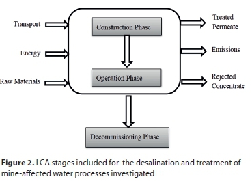
The function for both systems is identical, i.e., to produce potable water of a certain quality. The functional unit for this study was 1 kL of water at the specified standard for potable water produced over the lifespan of each process unit. The selection of this particular functional unit enabled a reference to which all inputs and outputs are related. It should be noted that this functional unit was chosen due to the demand for potable water. The mine-affected water would have had to be treated as per current South African guidelines before being released into the environment. However, the quality would have been required to meet a much lower standard as compared to that of potable water. For seawater there is no need for treatment in the absence of the potable water demand. For the purpose of this study the potential treatment of mine-affected water in the absence of potable water demand was neglected, as in reality the membrane processes would not have been employed if not for the need for potable water quality.

Data quality requirements are a general indication of the characteristics of the data for the study. For both case studies, data that were directly obtained from the feasibility and design reports were preferable. Such data included the consumption of electricity and chemicals. For process flows within the system that were not available, mass balances were employed. When direct data was unavailable, as was the case for the construction of civil engineering structures, calculations based on technical literature were utilised. Several calculations were often undertaken and the highest values, representing a worst-case scenario, were used for purposes of the study. Decisions regarding materials of construction as well as equipment types were based on case studies of similar water treatment processes. The geographical area for data gathering was South Africa. Within the SimaPro databases, South African data were only available for national electricity and mined coal that was used as filter media. For the remainder of the inputs, European or global figures were utilised.

Limitations to a certain extent were to be expected, considering the task of accounting for all inputs and outputs of the system. In general, data were found to be sparse and lacking which is often the case for LCAs, but even more so for industries based in South Africa. One problem that was encountered was that data were considered to be confidential and thus were not easily accessible. This was the case for both case studies and lengthy negotiations had to occur before any exchange of information happened. Agreements between Umgeni Water, Prentec and the consulting engineers had to be made in order to obtain certain process details. Another reason for the lack of data can be attributed in part to the fact that the desalination plant was still in the early design phases. Thus, some information, such as the weights of certain pumps, was unavailable. As a result, information from design specification sheets for similar pumps had to be used as inputs for the calculations. For the mine-water reclamation plant, design data rather than operational data had to be utilised. This was due to changes in the feed quality of the source water which affected the operation of the plant.

A set of assumptions had to be made in order to bridge data gaps. For certain inputs that were based on international data, it was assumed that the technology and equipment utilised will perform in a similar manner to what is used in South Africa. Where the material of construction was unspecified for components such as the filter cells, various literature sources were perused and the most common materials were selected for the purpose of calculation. In other instances, super duplex stainless steel was chosen as the construction material of choice for any equipment that is in contact with the ocean water. It was also assumed that both plants will be operational for the entire year, i.e. 365 days with no allowance for shutdown periods. This was to account for the worst-case scenario.

Inventory analysis

As the second stage of the LCA process, the inventory analysis consisted of collecting environmentally relevant data as well as formulating equations in order to quantify the flows into and out of the system. For this particular study, the process of data collection and compilation was the most work-intensive and time-consuming activity.

Data collection for the desalination plant

The procedure for data collection started off with a compilation of a process flow diagram (PFD) which highlighted the significant flows and operations within the system. From this point, a spreadsheet was drawn up which included material and energy inputs and outputs for each unit operation. For the construction phase, four major components were analysed: civil engineering structures, pipes, pumps, filters and membranes. Civil engineering structures consisted of fixtures such as tanks, pillars and filter cells. The weights of these constituents were generally not stated and had to be calculated based on available dimensions provided in the feasibility reports. In the event that the material of construction was not specified, technical literature was used to select the most appropriate building material.

In the case of pipes, all pipes were specified to be constructed of high density polyethylene (HDPE) due to its higher durability, non-corrosive nature and lower construction and maintenance costs compared to other materials. The mass of these pipes was calculated by firstly calculating volume of a hollow cylinder (which represents a pipe) using the inside and outside diameters, subtracting the volume of the inner from the outer and using the density to obtain the mass. The second method used a HDPE pipe brochure to obtain the mass of the pipe based on the outer diameter and standard dimension ratio (SDR) class which were stated in the Pipelines and Pump Stations Report (Umgeni Water, 2015b). The higher figure was then utilised in subsequent calculations.

Pumps are a fundamental part of the infrastructure of any plant and the design for the proposed desalination plant was no different. For the intake pumps, options were provided for various pump models in the above-mentioned report that detailed pipe specifications (Umgeni Water, 2015b). The mass was then obtained from locating the pump specification sheets for the selected model. For other pumps where model numbers were unavailable, the installed motor size and pumping capacity which was provided in the Desalination Options and Feasibility Report (Umgeni Water, 2015a) were used as guidelines to select an appropriate pump. The masses of the respective pumps were taken as a single entity inclusive of parts such as motors, gears, bearings, casings, etc. This was due to difficulty experienced in obtaining these figures. The Feasibility Report also detailed that the pumps be constructed of super duplex stainless steel. As such a material was not available on the SimaPro database, steel which had a high chromite content (±25%) was selected.

For the production of potable water, the main operational inputs into the system were the energy consumed, the chemicals utilised and the filter media, as displayed in Table 1. There were a range of chemicals used in the production process with the majority being used in the pre-treatment and post-treatment phase. Chemicals were used for various purposes: disinfection, RO membrane cleaning, chlorination and re-mineralisation. The utilisation of chemicals was stated in terms of milligrams per litre of water (mg/L) with the majority of the chemicals specified. For the chemicals that were not categorically stated, such as the coagulant and antiscalant, research was undertaken to determine the most suitable chemical for the application. Table 1 provides a summary of the chemical usage for the desalination process. The first and second column lists the chemicals mentioned in the Umgeni Water report as well as the unit operation. The last column states the chemical that was utilised in SimaPro based on technical literature.

 

 

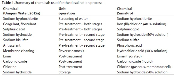
From the literature review, it is evident that the electricity requirement has always been one of the determining factors regarding life cycle assessment results. For the purposes of this study, this information was available in the Feasibility Report and was expressed in terms of kWh/m³ (Umgeni Water, 2015a). As electricity is such a fundamental element, it was imperative that a consistent and representative life cycle inventory (LCI) of electricity supply was utilised. The latest version of ecoinvent (version 3) offers new LCI data of power supply in 71 geographical locations which includes South Africa (Paul Scherrer Institute, 2012). Thus, this inventory set was utilised for this study to account for the South African energy mix.

The filtration step forms part of the pre-treatment phase to protect the RO membranes further on in the process. As mentioned in the previous sub-section, dual media filters were specified in both stages of pre-treatment containing silica sand, anthracite and garnet. SimaPro contains data for coal from extraction to point of sale in South Africa. This local dataset was utilised to represent the media layers for the filters.

Data collection for the mine-water reclamation plant

This procedure commenced with an initial meeting with the senior process engineer from Prentec. An overview of the treatment process was provided together with several process and instrumentation diagrams (PIDs) as well as schedules for power use. This was followed by the compilation of the spreadsheet that segregated the design data per unit operation and then further into the construction and operation phases. Average design feed flows into each sub-operation were stated in the design reports.

The major constituents of the construction phase for this case study comprised of components such as civil engineering structures, frames of the modules, grating, pipes, pumps, filters and membranes. The civil engineering structures for this case study consisted of tanks and filter cells. Design sheets for the various tanks provided dimensions of the tanks such as the diameters and heights. This was utilised to calculate the circumference and thereafter the number of panels that make up the wall of the tank. Together with the dimensions of the panel, the weight of the walls and base of the tank can be calculated. From the design sheets, the material of construction for the base and walls was reinforced concrete to withstand pressures of 25 and 30 MPa, respectively. With respect to working life, the senior process engineer was consulted and agreed that a reasonable working life for tanks would be 50 years.

For this case study, the mass of components, such as the frames of the skid, grating and pipes, were obtained courtesy of the personnel from the company involved. A 3D model of the plant, which collates the total mass of each skid, was utilised, from which masses of the individual items were extracted. These data are extremely accurate as pipe mass would include the mass of all lengths of pipe including all bends and tees. The frames and grating that form part of the skid are constructed of carbon steel and galvanised steel, respectively, while the pipes are either assembled from PVC or stainless steel. As advised by the design engineer, the working life of the frames, grating and stainless steel pipes was taken as 25 years while the PVC pipes were assumed to last 20 years.

With respect to the pumps, product names were provided in the design proposal report. As the majority of the pumps were manufactured by Grundfos, the product centre on the Grundfos website was perused. As all the pumps were classified as 'end suction close coupled' (NB range), the pump catalogue was browsed by pump design to locate the masses of the specific pumps. As in the initial case study, the masses of the respective pumps were taken as a single entity inclusive of all internal mechanical parts. The working life of all pumps was stated as 7 years.

The water treatment process for mine-affected water consists of two stages of treatment. Thus, there were two stages of reverse osmosis and two stages of ultrafiltration (UF). For the RO membranes, the masses of 8" spiral wound membranes were obtained from the Dow website while the design sheets for the glass-reinforced plastic vessels were provided. According to the engineer as well as figures from technical literature, the membranes which are constructed of polysulphone would last an average of 5 years while the working life of the outer shells was noted as 20 years. With respect to the UF membranes, product data sheets for the weight of membranes were located on the supplier's website. These were constructed of polyvinyl chloride (PVC) with the same working life as the RO membranes.

The three components in the operation phase include the chemical use within the process and the energy consumption as well as the filter media used. There were numerous chemicals used in the treatment process to satisfy various objectives. Amongst them were coagulants, biocides, antiscalants, chemically enhanced backwash (CEB) and clean-inplace (CIP) chemicals. The major chemical constituents used were phosphoric acid as an antiscalant, ferric chloride as a coagulant and secondary antiscalant, sodium hydroxide, sodium hypochlorite and hydrochloric acid as CEB and CIP chemicals. The average concentrations in terms of ppm for each chemical were provided.

From the literature, it was evident that energy was of utmost importance. Thus, a concerted effort was made to obtain an accurate portrayal of the electricity consumption within the process. The power used by each unit operation expressed as kilowatts was obtained from a design schedule. Together with the design feed rate into each area, the electricity requirement in terms of kWh/m³ was calculated. As with the first case study, the South African electricity (medium voltage) dataset in SimaPro was utilised.

To fulfil the purpose of pre-treatment, DUP filters were employed prior to the membrane treatment stages. The filter media consisted of two layers: silica sand and magnetite. As in the case of the desalination process, the local data available in SimaPro were utilised to represent both media layers for the filtration process.

Input into SimaPro

For an effective assessment, all data had to be scaled down in accordance with the functional unit. Thus, all material data were expressed in terms of kg/kL potable water, energy inputs as kWh/kL potable water and chemicals used as mg/kL potable water. Once this information was in the relevant format, it could be used as inputs into the SimaPro LCA Software. Within the SimaPro programme, new projects depicting both processes were created. In addition, each unit operation was developed as an individual process together with the appropriate inputs and outputs.

The result of the inventory analysis was the generation of an inventory table. This is as a result of the 'analyse' function used in SimaPro which, through a reduced matrix, calculates the system inventory by constructing the process network and tracing the movement of materials from one stage to another. The software presents the table as a single list that is itemised alphabetically. This list is used as an input into the following phase, the impact assessment phase, which seeks to understand the contribution of the various processes to the overall environmental burden.

Impact assessment

The impact assessment phase aims to establish a link between the product system and potential environmental impacts. To achieve this objective, inventory information is related to relevant impact categories and indicators. Furthermore, this phase provides a basis for the next stage, i.e., life cycle interpretation.

The ISO 14042 (2000) document stated that there are three compulsory steps that need to be completed: selection and definition of impact categories, classification and characterisation. In addition, there are several optional elements that can be used, dependent on the goal and scope of the study: normalisation, grouping, weighting and data quality analysis. For the purposes of this study, the three mandatory elements were deemed sufficient and were thus performed for the system. The optional steps were excluded to avoid introducing a degree of subjectivity to the study.

The SimaPro 8.1.1.16 Software contains various impact assessment methods. For the study, the ReCiPe Midpoint Method was used. At this level, 18 impact categories are defined: climate change, human toxicity, ionising radiation, photochemical oxidant formation, particulate matter formation, terrestrial acidification, ozone depletion, terrestrial ecotoxicity, agricultural land occupation, urban land occupation, natural land transformation, marine ecotoxicity, marine eutrophication, fresh water eutrophication, fresh water ecotoxicity, fossil fuel depletion, minerals depletion and fresh water depletion. The full set of 18 impact categories has been used due to availability and completeness.

Interpretation

As the final stage in the LCA study, the interpretation phase aims to analyse the results from the previous phase and draw appropriate conclusions and recommendations.

For the interpretation phase, one kL (m³) of potable water for distribution was analysed by the ReCiPe method. As data were collected pertaining to the construction and operation phases, it was decided to firstly segregate the environmental impacts in terms of these two phases. This was possible through the 'analyse groups' function in SimaPro which provides the user with an opportunity to select and compare the impact of various operations or inputs in terms of the available categories. The results were presented in a tabular format which provided an overview of the contributions of the individual sub-processes. In addition, each impact category was also examined in greater detail with the results depicted in a network diagram which produces a visual representation of each input's contribution to the overall impact of the process.

 

RESULTS

The analysis of the results obtained from the study form part of the final phase of the LCA methodology which is Life Cycle Interpretation. The resulting evaluation would be utilized to reach suitable conclusions and provide relevant recommendations.

Results for the desalination process

Figure 3 illustrates the contribution of the various inputs to the relevant impact categories that are pre-defined in the software package as part of the ReCiPe impact assessment method. From the diagram, it is evident that electricity has an overwhelming burden contribution in 11 of 18 of the categories, such as climate change and terrestrial acidification. However, in other categories such as water, ozone and minerals depletion, the contribution of electricity is much lower (approximately 40 to 50%) and as low as 25% for agricultural land occupation, with the chemical usage becoming more prominent. It is also interesting to note that the infrastructure carries a relatively insignificant burden compared to the other two inputs.

 

 

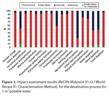
For the mine-water reclamation process (Fig. 4), electricity consumption has the greatest contribution to the bulk of the impacts. In the case of impact categories such as climate change and terrestrial acidification, the energy usage is responsible for greater than 95% of the overall impact. In the case of other impacts, e.g., ozone and metal depletion, chemical consumption within the water treatment process carries a much more significant environmental burden as it accounts for approximately half of the total impact. The results also indicate that chemical usage had a positive environmental impact on agricultural land occupation. This is due to the use of two chemicals, ferric chloride and hydrochloric acid, attributed to the manufacture of chlorine and associated use of wood chips. Unlike the operation phase, the environmental impact of the infrastructure phase, which encompasses materials used in the construction of the plant, is relatively less significant.

 

 

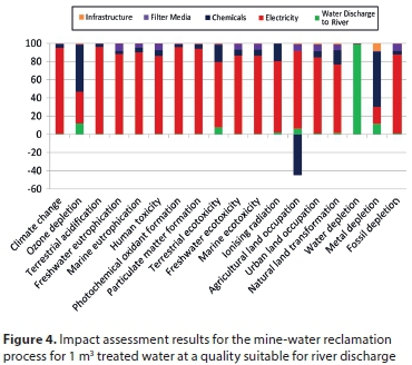
Desalination and mine-water reclamation environmental scores

Once the results for the individual categories for each case study had been analysed, a comparison between the two water treatment processes was made. Table 2 provides a summary of the total environmental impacts. The figures highlight the fact that the desalination process carries a much higher overall burden compared to the mine-water reclamation process. For the bulk of the categories such as climate change and terrestrial acidification, desalination displays scores that are approximately double the impact associated with mine-water reclamation. There are two categories where mine-water reclamation performs worse than desalination: water and metal depletion. This can be attributed to the process of extracting the groundwater from abandoned mines, thereby adversely affecting the water and metal content in the surrounding environment. Furthermore, the significant depletion of water for the mine-water reclamation process is mainly due to the source water. In the case of desalination, the impact assessment method utilized does not consider water depletion of seawater. Hence, the figure for overall water depletion for desalination is significantly lower then that for mine-water reclamation. These assumptions mirror the water situation in the country - the scarcity of fresh water in general, and the abundance of seawater for costal cities in South Africa.

 

 

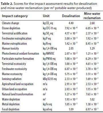
Although a comparison between the water treatment processes can be made, there are associated challenges and difficulties as the operations differ in many respects. Table 3 highlights a few of the significant differences between the two processes. The ISO 14040 (2006) document states that the results of various LCA studies can only be directly compared if the assumptions and context of each study are the same.

Both the water treatment processes discussed in the study are secondary processes which are necessary to implement due to the scarcity of water. In addition, there are also practical considerations that need to be taken into account prior to the design of these plants. Due to its feed source, the desalination plant has to be constructed in coastal areas with close proximity to seawater. As the mine reclamation plant will have to treat accumulated water from previously mined areas, the plant will reside close to the mines. The feed water quality for mine-water reclamation is also a significant factor due to variances in source water. This occurs as a result of different minerals being mined as well as the age of the mine. The quality of the mine-water to be treated is the main factor why the results for the current mine-water cannot be generalised to other mine-affected waters from other locations and/or mines.

Energy requirements and the potential for improvement

Energy consumption is an important cost and environmental factor for all water treatment processes, and especially for desalination. Therefore, benchmarking energy consumption is of value. In South Africa, it has been proposed that electricity consumption be used as a crude environmental indicator for the performance of urban water systems (Friedrich et al., 2009). In terms of energy requirements, seawater membrane desalination with energy recovery devices generally consumes about 3.5-4.5 kWh/m³ of electricity according to Vince et al. (2008) and between 4 to 6 kWh/m³ according to Abdelkareem et al. (2017). The desalination of brackish water needs about 1.5 to 2.5 kWh/m³ (Abdelkareem et al., 2017). The local desalination process investigated in this study should need a total of 3.69 kWh/m³ which is within the above-mentioned ranges. Furthermore, it is lower than the stated electricity consumption of the three operational desalination plants in South Africa: the Sedgefield Plant (3.97 kWh/m³), the Albany Coast Plant (4.52 kWh/m³) and the Mossel Bay Plant (4.39 kWh/m³) (Turner et al., 2015). However, this figure has to be validated and monitored once the desalination plant will become operational.

A further assessment regarding energy consumption was undertaken comparing the environmental impacts of alternative water treatment plants to a conventional water treatment plant in South Africa. At the outset, it must be acknowledged that the energy requirement for desalination and mine-water reclamation is much greater than other water treatment technologies. When considering the conventional treatment of raw wastewater in the local context, the Wiggins Waterworks had the highest electricity consumption per kilolitre of water produced at 0.10 kWh/m³ which represents the worst-case scenario for the eThekwini Municipality (Friedrich et al., 2009). The total energy consumption of the proposed desalination plant is 3.69 kWh/m³ and 2.16 kWh/m³ for the mine-water reclamation plant. Taking the above two figures for energy usage and associating them with characterisation factors for climate change due to the use of renewable energy sources (sun and wind) yields the results in Table 4. In addition, the South African 2030 electricity mix as described in the Integrated Resource Plan - Scenario IRP 1 (DoE) 2018) was modelled to represent a realistic situation for the future energy requirement of both water treatment plants. This scenario assumes that by 2030 the South African electricity mix will be from coal (64%), wind (13%), solar energy (8%), nuclear energy (4%), hydro energy (3%), gas (1%) and others (5%). It is the most conservative scenario presented in the planned integrated resource plan for South Africa (DoE, 2018). Although less than 1% of the RO desalination plants worldwide are currently powered by renewable sources, their use is predicted to increase in the future (Abdelkareem et al., 2017).

The figures in Table 4 demonstrate that desalination using wind and solar power has the potential to produce GHG emissions in the range of 0.07-0.28 kg CO₂ eq/kL potable water. The release of GHG emissions for the mine-water reclamation plant will be even lower with emissions between 0.04 and 0.16 kg CO₂ eq/kL potable water. These figures are comparable to the emissions of 0.08-0.11 kg CO₂ eq/kL water, which would be released from the conventional water treatment processes employed at Durban Heights and Wiggins Waterworks. These are the two most important Umgeni Water potable water plants in the eThekwini Municipality (core city Durban).

The figures in Table 4 for renewable energy sources represent an ideal best-case scenario which in reality cannot be achieved by membrane plants of the sizes of those investigated in this study. Large RO plants usualy need storage and backup and, therefore, practically cannot rely 100% on renewable energy. However, in the literature a series of authors (Biswas et al., 2009; Stokes et al., 2009 and Shahabi et al., 2014) have used 100% wind energy and 100% solar energy for similar studies involving RO in order to gauge a best-case scenario. From an implementation and practical point of view, Chew and Ng (2019) also used 100% solar power in this manner for a small pilot plant for ultra-filtration membranes to be used for rural (off-grid) water supply in Malaysia. In the South African context this is an unrealistic best-case scenario which can only be theoretically considered for plants of the size of those investigated in this study.

The South African 2030 electricity mix (64% coal, wind 13%, solar 8%, nuclear 4%, hydro 3%, gas 1% and other 5%) was modelled to represent a realistic situation for the future energy requirement of membrane-based plants in South Africa. Results indicate that that desalination using the predicted 2030 energy mix has the potential to produce 1.16 kg CO₂ eq/ kL potable water. The release of GHG emissions for the mine-water reclamation plant will be even lower at 0.678 kg CO₂ eq/kL potable water. This shows that a reduction in coal-fired energy coupled with an increase in the use of renewable energy sources has the potential to decrease the carbon footprint of water treatment plants that use alternative feed sources. These are more realistic calculations for the local context.

The results presented in Table 4 are in line with similar results from other studies. For example, Raluy et al. (2004) reported that a reduction of greater than 35% is expected, dependent on the origin of the energy, i.e., cogeneration, internal combustion engine or a combined cycle (Raluy et al., 2004). In a follow-up report, Raluy et al. (2005) has reported that, for a desalination plant using an energy source that is based on combustion of fossil fuel, carbon dioxide emissions of 1.78 kg/m³ of desalted water and NOx emissions of 4.05 g/m³ of desalted water were released. Together with the integration of the RO system with photovoltaic energy, CO₂ emissions were reduced to between 0.6 and 0.9 kg/m³ eq. and NOx emissions to between 1.8 and 2.1 g/m³ (Raluy et al., 2005). A further decrease in environmental impact is achieved when wind energy is utilised in conjunction with the desalination plant with CO₂ emissions of 0.1 kg/m³ eq and NOx emissions of 0.4 g/m³ (Raluy et al., 2005). Biwas (2009) reports for Western Australia a potential reduction of CO₂ emissions from 3.80 kg/ m³ (electricity mix) to 0.32 kg/ m³ (100% wind power) due to the replacement of conventional electricity by wind power. Stokes and Horvath (2009) show a similar trend for California where CO₂ emissions were potentially reduced from 3.95 kg/ m³ to 0.72 kg/ m³ by replacing the US average electricity mix with 100% photovoltaic electricity. Thus, a substantial reduction in emission of GHG is theoretically possible by substituting fossil fuels with renewable energy sources. Another emerging renewable energy source not investigated in this research but appropriate for the desalination plant is the energy from ocean waves (Leijon and Boström, 2017).

Other available options to reduce the energy usage of a membrane-based water treatment plant include the implementation of a hybrid system which incorporates both brackish and seawater elements as well as a two-pass NF system (Veerapaneni et al., 2007 and Long, 2008). Investigation into innovative material based membranes that reduce fouling are also currently underway (Subramani et al., 2011). In addition, emerging technologies such as forward osmosis, ion concentration polarization and capacitive deionization technology are all advancements in the pipeline that could potentially have a positive impact on energy consumption (Elimelech and Phillip, 2011 and Subramani et al., 2011).

Chemical requirements and the potential for improvement

Chemical production and use also carries a significant burden for both case studies. In particular, the chemicals for post-treatment (lime and carbon dioxide) in the desalination process and for pre-treatment (ferric chloride as coagulant, secondary antiscalant and biocide) in the mine-water reclamation process appear in the modelling process as the chemicals with the highest impacts. This is in line with results reported by Vince et al. (2008). Large doses of chemicals are necessary in order to adjust the alkalinity of the demineralised water to potable water quality standards. For the selected desalination process, lime and CO₂ release the highest amount of GHG emissions after electricity use. These results necessitate an investigation into alternate chemicals as well as permeate blending of the product water with other mineralised water sources in order to decrease chemical use.

Vince et al. (2008) carried out an analysis centred around various water treatment processes for particular local conditions. One of the conclusions that was reached pertains to the detrimental effect of coagulant production and use (Vince et al., 2008). As is evident from the treatment of mine-water, the usage of coagulant depends on the concentration of organic and suspended matter in the source water. Vince et al. (2008) goes on to state that the production of a kilogram of ferric chloride has an impact on ozone depletion that is equal to the impact of 35 kg of aluminium sulphate. This brings to light the fact that the choice of similar chemicals may result in vastly different impacts. For the second case study, ferric chloride is responsible for 35% of the total potential for ozone depletion of the system. Thus, it is recommended that the production process of ferric chloride be investigated together with the consideration of other coagulants. In addition, it has been proven by Al-Mashharawi et al. (2012) that the use of low-pressure membranes in the pre-treatment phase has the capacity to reduce the use of coagulants. This should be also considered for the local desalination case study.

As far as the toxicity of discharged concentrate is concerned, Mezher et al. (2011) mentions that the overall temperature, density and total dissolved salts (TDS) of the discharge are of importance as they could potentially cause damage to the aquatic ecosystem. Increased temperature could have detrimental consequences while a rise in specific gravity would cause the contents of the reject stream to sink. The quantity of dissolved solids also increases with an increase in plant recovery. These factors need to be considered when debating the release of any concentrate into large bodies of water.

 

CONCLUSIONS

The results indicate that the operational phase is the predominant stage responsible for the majority of the environmental impacts attributed to both systems. Within this stage, the energy consumption is generally the greatest contributor, with chemical use representing the second-highest environmental burden. A detailed investigation of both water treatment processes reveals that the desalination process has a greater overall environmental impact than the mine-water reuse process, mainly due to the increased energy requirements. As the results indicate that plant impacts are highly dependent on the electricity supply source, further investigations of the substitution of fossil fuel-based energy with renewable energy were undertaken. It was calculated that the use of solar or wind energy could significantly reduce the climate change effect (i.e. reduce GHG emissions) of using seawater and mine-affected water to levels that are comparable to conventional water treatment processes currently employed in the eThekwini Municipality. Other technological developments should also be considered to reduce the energy and chemical usage of the system and can bring environmental improvments, in particular for the desalination plant as it is still in the planning process. In particular for this plant a pre-treatment stage and an overall optimization with regard to chemical usage should be investigated, as well as replacing chemicals with high environmental burdens. For long-term future developments of the RO processes for the production of potable water, the use of alternative sources of energy (solar and wind) should be promoted.

 

ACKNOWLEDGEMENTS

The authors would like to acknowledge the Water Research Commission for sponsorship of this study and Umgeni Water as well as Prentec for the provision of information.

 

REFERENCES

ABDELKREEM MA, ASSAD MEH, SAYED ET and SOUDAN B (2017) Recent progress in the use of renewable energy sources to power water desalination plants. Desalination 435 97-113. https://doi.org/10.1016/j.desal.2017.11.018        [ Links ]

AL-MASHHARAWI S, GHAFFOUR N, AL-GHAMDI M and AMY G (2013) Evaluating the efficiency of different MF and UF membranes used as pretreatment for Red Seawater RO desalination. Desalin. Water Treat. 51 617-626. https://doi.org/10.1080/19443994.2012.699449        [ Links ]

BARJOVEANU G, COMANDARU IM and TEODOSIU C (2010) Life cycle assessment of water and wastewater treatment systems: an overview. Bull. Polytech. Inst. Iasi 56 73-86.         [ Links ]

BISWAS WK (2009) Life cycle assessment of sea water desalination in Western Australia. World Acad. Sci. Energ. Technol. 56 369-375.         [ Links ]

BUCKLEY CA, FRIEDRICH E and VON BLOTTNITZ H (2011) Life cycle assessments (LCA) in the south african water sector: a review and future challenges. Water SA 37 (5) 718-726. https://doi.org/10.4314/wsa.v37i5.9        [ Links ]

CHEW CM and NG KMD (2019) Feasibility of solar-powered ultrafiltration membrane water treatment systems for rural water supply in Malaysia. Water Supply 19 (6) 1758-1766. https://doi.org/10.2166/ws.2019.050        [ Links ]

DOE (Department of Energy, South Africa) (2018) Integrated Resource Plan. URL: http://www.energy.gov.za/IRP/irp-update-draft-report2018/IRP-Update-2018-Draft-for-Comments.pdf (Accessed February 2019).         [ Links ]

DWA (Department of Water Affairs, South Africa) (2013) National Water Resources Strategy. Department of Water Affairs, Pretoria, South Africa.         [ Links ]

DOW FILMTEC (2015) Dow Filmtec Element. Dow Filmtec, United States of America.         [ Links ]

ELIMELECH M and PHILLIP WA (2011) The future of seawater desalination: energy, technology, and the environment. Science 333 712-717. https://doi.org/10.1126/science.1200488        [ Links ]

EUROPEAN COMMISSION (2010) International Reference Life Cycle Data System (ILCD) Handbook: General guide for Life Cycle Assessment - Detailed guidance. European Union, Ispra, Italy.         [ Links ]

FRIEDRICH E (2002) Life-cycle assessment as an environmental management tool in the production of potable water. Water Sci. Technol. 46 (9) 29-36. https://doi.org/10.2166/wst.2002.0198        [ Links ]

FRIEDRICH E, PILLAY S and BUCKLEY CA (2009) Environmental life cycle assessments for water treatment processes - A South African case study of an urban water cycle. Water SA 35 (1) 73-84. https://doi.org/10.4314/wsa.v35i1.76710        [ Links ]

GOLDER ASSOCIATES AFRICA (2012) Environmental Impact Assessment (EIA) for the Proposed Water Reclamation Scheme - Draft Environmental Impact Assessment. Golder Associates Africa, Johannesburg.         [ Links ]

HYDRANAUTICS (2016) Capillary Ultrafiltration Module. Lentech, Delft, The Netherlands.         [ Links ]

LEIJON J and BOSTRÖM C (2017) Freshwater production from the motion of ocean waves. Desalination 435 161-171. https://doi.org/10.1016/j.desal.2017.10.049        [ Links ]

ISO (2006) ISO 14040: Environmental Management - Life Cycle Assessment - Principles and Framework. International Organisation for Standardisation, Geneva.         [ Links ]

ISO (2000) ISO 14042: Environmental Management - Life Cycle Assessment - Life Cycle Impact Assessment. International Organisation for Standardisation, Geneva.         [ Links ]

KNÜPPE K (2011) The challenges facing sustainable and adaptive groundwater management in South Africa. Water SA 37 (1) 67-79. https://doi.org/10.4314/wsa.v37i1.64110        [ Links ]

LONG B (2008) Optimisation of desalination for low energy. Singapore International Water Week, Singapore.         [ Links ]

LOUBET P, ROUX P, LOISEAU E AND BELLON-MAUREL V (2014) Life cycle assessments of urban water systems: A comparative analysis of selected peer-reviewed literature. Water Res. 67 187-202. https://doi.org/10.1016/j.watres.2014.08.048        [ Links ]

MEIER K (2012) Infrastructure Master Plan: Chapter 4.5 Wastewater reuse. Umgeni Water, Pietermaritzburg, South Africa.         [ Links ]

MEIJERS K, VERBERNE AJP and KOREMAN EA (1998) Levens-cyclusanalyse van membraanfiltraatie. H2O 21 33-36.         [ Links ]

MEZHER T, FATH H, ABBAS Z and KHALED A (2011) Techno-economic assessment and environmental impacts of desalination technologies. Desalination 266 (1) 263-273. https://doi.org/10.1016/j.desal.2010.08.035        [ Links ]

PAUL SCHERRER INSTITUTE (2012) Electricity generation & supply in ecoinvent v3. URL: https://www.ecoinvent.org/files/201206_bauer_electricity_in_ecoinvent_v3.pdf (Accessed 1 June 2016).         [ Links ]

PRENTEC (2013) Proposal for low waste mine water treatment plant. Prentec, Johannesburg, South Africa.         [ Links ]

RALUY GR, SERRA L and UCHE J (2005) Life cycle assessment of water production technologies Part 1: Life cycle assessment of different commercial desalination technologies (MSF, MED, RO). The Int. J. Life Cycle Assess. 10 285-293. https://doi.org/10.1065/lca2004.09.179.1        [ Links ]

RALUY R, SERRA L, UCHE J and VALERO A (2004) Life-cycle assessment of desalination technologies integrated with energy production systems. Desalination 167 445-458. https://doi.org/10.1016/j.desal.2004.06.160        [ Links ]

RAS C and VON BLOTTNITZ H (2012) A comparative life cycle assessment of process water treatment technologies at the Secunda Complex. Water SA 38 (4) 549-554. https://doi.org/10.4314/wsa.v38i4.10        [ Links ]

SHAHABI MP, McHUGH A, ANDA M and HO G (2014) Environmental life cycle assessment of seawater reverse osmosis desalination plant powered by renewable energy. Renew. Energ. 67 53-58. https://doi.org/10.1016/j.renene.2013.11.050        [ Links ]

STOKES JR and HORVATH A (2009) Energy and air emissions effects of water supply. Environ. Sci. Technol. 43 2680-2687. https://doi.org/10.1021/es801802h        [ Links ]

SUBRAMANI A, BADRUZZAMAN M, OPPENHEIMER J and JACANGELO JG (2011) Energy minimization strategies and renewable energy utilization for desalination: A review. Water Res. 45 1907-1920. https://doi.org/10.1016/j.watres.2010.12.032        [ Links ]

TURNER K, NAIDOO K, THERON J and BROODRUK J (2015) Investigation into the cost and operation of Southern African desalination and water reuse plants. WRC Report No. TT 636/15. Water Research Commission, Pretoria.         [ Links ]

UMGENI WATER (2015a) KwaZulu-Natal East Coast Desalination Plants, Detailed Feasibility Study, Pipelines and Pump Stations Report. Umgeni Water, Pietermaritzburg, South Africa.         [ Links ]

UMGENI WATER (2015b) KwaZulu-Natal East Coast Desalination Plants, Detailed Feasibility Study, Desalination Options and Feasibility Report. Umgeni Water, Pietermaritzburg, South Africa.         [ Links ]

VEERAPANENI S, LONG B, FREEMAN S and BOND R (2007) Reducing energy consumption for desalination. J. Am. Water Works Assoc. 99 (6) 95-106. https://doi.org/10.1002/j.1551-8833.2007.tb07958.x        [ Links ]

VINCE F, AOUSTIN E, BRÉANT P and MARECHAL F (2008) LCA tool for the environmental evaluation of potable water production. Desalination 220 (1-3) 37-56. https://doi.org/10.1016/j.desal.2007.01.021        [ Links ]

ZHOU J, CHANG V W-C and FANE AG (2014) Life cycle assessment for desalination: A review on methodology feasibility and reliability. Water Res. 60 210-223. https://doi.org/10.1016/j.watres.2014.05.017        [ Links ]

 

 

Received 26 April 2018
Accepted in revised form 25 September 2019

 

 

* Corresponding author, email: Friedriche@ukzn.ac.za

^rND^sABDELKREEM^nMA^rND^sASSAD^nMEH^rND^sSAYED^nET^rND^sSOUDAN^nB^rND^sAL-MASHHARAWI^nS^rND^sGHAFFOUR^nN^rND^sAL-GHAMDI^nM^rND^sAMY^nG^rND^sBARJOVEANU^nG^rND^sCOMANDARU^nIM^rND^sTEODOSIU^nC^rND^sBISWAS^nWK^rND^sBUCKLEY^nCA^rND^sFRIEDRICH^nE^rND^sVON BLOTTNITZ^nH^rND^sCHEW^nCM^rND^sNG^nKMD^rND^sELIMELECH^nM^rND^sPHILLIP^nWA^rND^sFRIEDRICH^nE^rND^sFRIEDRICH^nE^rND^sPILLAY^nS^rND^sBUCKLEY^nCA^rND^sLEIJON^nJ^rND^sBOSTRÖM^nC^rND^sKNÜPPE^nK^rND^sLOUBET^nP^rND^sROUX^nP^rND^sLOISEAU^nE^rND^sBELLON-MAUREL^nV^rND^sMEIJERS^nK^rND^sVERBERNE^nAJP^rND^sKOREMAN^nEA^rND^sMEZHER^nT^rND^sFATH^nH^rND^sABBAS^nZ^rND^sKHALED^nA^rND^sRALUY^nGR^rND^sSERRA^nL^rND^sUCHE^nJ^rND^sRALUY^nR^rND^sSERRA^nL^rND^sUCHE^nJ^rND^sVALERO^nA^rND^sRAS^nC^rND^sVON BLOTTNITZ^nH^rND^sSHAHABI^nMP^rND^sMcHUGH^nA^rND^sANDA^nM^rND^sHO^nG^rND^sSTOKES^nJR^rND^sHORVATH^nA^rND^sSUBRAMANI^nA^rND^sBADRUZZAMAN^nM^rND^sOPPENHEIMER^nJ^rND^sJACANGELO^nJG^rND^sVEERAPANENI^nS^rND^sLONG^nB^rND^sFREEMAN^nS^rND^sBOND^nR^rND^sVINCE^nF^rND^sAOUSTIN^nE^rND^sBRÉANT^nP^rND^sMARECHAL^nF^rND^sZHOU^nJ^rND^sCHANG V^nW-C^rND^sFANE^nAG^rND^1A01^nAmy^sdu Pisanie^rND^1A01^nLouis^sdu Preez^rND^1A01^nJohnnie^svan den Berg^rND^1A01^nRialet^sPieters^rND^1A01^nAmy^sdu Pisanie^rND^1A01^nLouis^sdu Preez^rND^1A01^nJohnnie^svan den Berg^rND^1A01^nRialet^sPieters^rND^1A01^nAmy^sdu Pisanie^rND^1A01^nLouis^sdu Preez^rND^1A01^nJohnnie^svan den Berg^rND^1A01^nRialet^sPieters

SHORT COMMUNICATION

 

The rate of release of Cry1Ab protein from Bt maize leaves into water

 

 

Amy du Pisanie; Louis du Preez; Johnnie van den Berg; Rialet Pieters^*

Unit for Environmental Sciences and Management, North-West University, Potchefstroom, 2531, South Africa

 

 

---

ABSTRACT

Transgenic Bt maize plants are genetically modified to contain genes of Bacillus thuringiensis that encode for δ-endotoxins (Cry1Ab protein) that have insecticidal properties. These endotoxins target certain lepidopteran pests of maize. There are several entry routes by which Cry proteins enter the aquatic ecosystem in which aquatic organisms are exposed to these proteins. The main route is through plant debris such as leaves, stalks and postharvest detritus that are transported by means of run-off, rain and wind. While several studies have been conducted on the fate of Cry1Ab protein in terrestrial ecosystems, little is known of the release rates of Cry1Ab proteins from maize plant tissues that end up in aquatic ecosystems. In this study, leaves of Bt-maize and its isoline were submerged in containers filled with deionised or borehole water for a period of 16 days, and kept at 3 different temperatures (10±1, 21±1 and 30±1°C). Samples were collected at 1, 2, 4, 8, 16, 24, 48, 96, 192 and 384 h post submersion and analysed for Cry protein content using enzyme-linked immunosorbent assay (ELISA). The release of Cry protein from submerged maize leaves was influenced by temperature, and duration of immersion. An increase in Cry protein levels in the water was observed from the first hour onwards in both water types until the end of the experiment. The highest concentration of Cry protein was found at 30°C. This study showed that temperature and time period influence the release rate of Cry proteins from dried leaf matter into the aquatic environment.

Keywords: aquatic ecosystem, arthropods, GM crops, environment, risk assessment

---

 

 

INTRODUCTION

Genetically modified (GM) transgenic Bt maize plants contain genes of the soil bacterium Bacillus thuringiensis that encode for δ-endotoxins (Cry1Ab protein) that have insecticidal properties. These endotoxins target certain lepidopteran pests of maize (Betz et al., 2000; Baumgarte and Tebbe, 2005; Bravo et al., 2007; Chambers et al., 2010). Production of Cry endotoxins by GM plants confers pesticidal properties to these plants, for example, Bt maize, of which various maize hybrids express different Cry proteins such as Cry1Ab, Cry1Ac and Cry1F, that are toxic for specific insect species (Baumgarte and Tebbe, 2005; Bravo et al., 2007; Swan et al., 2009). While GM Bt maize that expresses only Cry1Ab protein has been planted in South Africa from 1998 onwards, Bt maize hybrids that express both Cry1.105 and Cry2Ab2 proteins started to replace these hybrids from 2012 onwards. South Africa is currently the 9^th largest producer of Bt maize in the world, with approximately 1.9 million ha planted to Bt crops in 2017 (ISAAA, 2017). The most Bt maize planted per country in 2017 was the 29.4 million ha in the USA and almost 15 million ha in Brazil (second-most). Globally, a combined surface area of 101 million ha is planted to Bt cotton, Bt maize and Bt soybean (ISAAA, 2017).

Between 65 and 75% of the maize planted annually in South Africa is Bt maize (Masehela et al., 2016), which is planted for control of the maize stem borer complex that consists of Busseola fusca (Lepidoptera: Noctuidae), Chilo partellus (Lepidoptera: Crambidae) and Sesamia calamistis (Lepidoptera: Noctuidae) (Van den Berg and Van Wyk, 2007; Van den Berg et al., 2013). The high adoption rates for Bt crops in the world are ascribed to the many benefits they provide to farmers. Reduced use of chemical insecticides, increased target specificity and ease of crop management are widely reported to be the drivers of these high levels of adoption (Raybould and Quemada, 2010; Kruger et al., 2009; Brookes and Barfoot, 2014). However, these crops have largely not been approved for cultivation in Europe and most countries in Africa. The benefits these crops hold are strongly debated, leading to controversies regarding environmental safety and effects on biodiversity (Naranjo, 2009; Lövei and Arpaia, 2005) and especially aspects around aquatic ecosystem health (Venter and Bøhn, 2016). It is especially with regards to aquatic environments where risk assessments are lacking (Carstens et al., 2012). Despite growing recognition that aquatic ecosystems near agricultural fields receive significant amounts of run-off and crop residues that contain these toxins (Böttger et al., 2015; Li et al., 2013), environmental risk assessments tend to neglect aquatic ecosystems as a relevant context for assessing the potential risks associated with GM crops.

A critical evaluation of the fate of Cry proteins is imperative in order to gain an accurate characterization of exposure levels to sensitive species for risk assessments. Arthropods that feed on Bt crop tissue ingest Bt protoxins which are then activated before they can have an effect on susceptible individuals (Broderick et al., 2006). The gut protease of the target pest species cleaves the protoxin producing an active toxin which binds to the mid-gut epithelial cells, creating pores in the cell membrane. This causes immobilization of the gut, lyses of epithelial cells and ultimately death due to both septicaemia and starvation (Broderick et al., 2006).

Direct exposure to Cry proteins takes place when transgenic crop residues are consumed by organisms (Kratz et al., 2010), while indirect exposure may be through leaching of protein from crop plant tissue into the aquatic environment, with possible adverse effects on exposed organisms (Li et al., 2007; Venter and Bøhn, 2016). There are several routes through which Cry proteins enter the aquatic ecosystem in which aquatic organisms are exposed to these proteins through different exposure pathways (Carstens et al., 2012). Rosi-Marshall et al. (2007) indicated the main entry route into aquatic systems to be through plant debris (which includes pollen, leaves, crop dust, stalks and postharvest detritus) that are transported by means of run-off, rain and wind. The leaching of Cry proteins from plant tissue can be influenced by temperature, plant tissue type, sediment composition and the presence of microbes (Li et al., 2007).

The presence and persistence of Cry1Ab protein in the environment has been studied by several authors. Bøhn et al. (2008) showed that Cry1Ab protein is present in maize grain at a concentration of approximately 67 ng/g tissue, and 2 530 ng/g in leaves (Holderbaum et al. 2015), and for stacked events the concentration can be much higher. The Bt toxin load in pollen of 'Smartstax' can be 100 to 200 ng/mg pollen dry mass (Phillips, 2008; Stillwell and Silvanovich, 2008). A study by Tank et al. (2010) indicated that the presence of Cry1Ab protein in natural streams containing maize detritus was above the minimum detection limit of 6 ng/L in 23% of the sites sampled.

In terrestrial ecosystems the concentration of Bt toxins in soil depends on soil type (Palm et al., 1994). Higher clay and organic matter results in stronger toxin binding, making extraction difficult (Palm et al., 1994). For example, 27% and 60% B. thuringiensis var. kurstaki (Btk) toxins were recovered from soil by Palm et al. (1994), with high and low clay-organic matter content, respectively. The degradation rate of Cry1Ab proteins in different soil types (differed in texture but not in silt or pH) showed that carbon dioxide (CO₂) production in soil was initially high and then declined over a period of 135 days, indicating that the Cry protein was used by microorganisms as a growth substrate (Valldor et al., 2015). The latter study also reported that the low levels of Cry1Ab in soil indicate that these proteins mineralize faster due to microbial degradation (Valldor et al., 2015). Cry toxin may also remain active in the soil where it binds quickly and tightly to humic acid and clays (Saxena et al., 1999; Carstens et al., 2012). Though bound, the Cry toxin maintains its insecticidal characteristic and, since it is bound to soil particles, is protected from degradation. Depending on the soil type, the toxin can persist for at least 234 days (Saxena et al., 1999).

Using an enzyme-linked immunosorbent assay (ELISA) to determine Cry1Ab levels, Zwahlen et al. (2003) studied how long the toxin remains in the plant tissue when left on field after harvest and over different periods of the year. They reported the degradation rate of Cry protein to be temperature dependent and reduced at lower soil temperatures. Feng et al. (2011) also reported that soil temperature had a significant effect on the degradation of Cry1Ab protein, but that pH had no obvious effect.

Jensen et al. (2010) reported that Cry1Ab protein present inside maize leaves lost its bioactivity after 2 weeks of immersion in water. However, they did not quantify the level of Cry1 proteins either in the plant tissue or aquatic medium, which made it difficult to determine whether the protein in the plant tissue degraded or leached out into the water. Another study reported a decline of Cry3Bb1 content in maize tissue following water immersion (Prihoda and Coats, 2008).

Cry proteins enter aquatic systems by leaching into the soil from plant material (Victorov, 2011). Leaf detritus are also left on fields to provide nutrition and as animal feed, while at the same time Bt proteins can leach into the ground and make its way to nearby streams or water bodies (Swan et al., 2009; Chambers et al., 2010; Carstens et al., 2012). Large amounts of maize debris have been reported to end up in water systems over very short periods of time (<7 days) (Victorov, 2011; Venter and Bøhn, 2016), which may lead to sudden increases in Bt protein concentration in such aquatic systems. The amount of Bt maize debris in water streams has been reported to correlate with the amount of Cry protein found in stream water (Tank et al., 2010). Whiting et al. (2014) reported high concentrations (33 ng/L) of Cry1Ab protein in run-off water sampled in maize fields. Shogren et al. (2019) found that Cry1Ab proteins are removed from the water column in riverine systems either via sorption of the protein to the biofilm or by biological removal thereof.

This study investigated the release rate of the Cry1Ab protein from water-submerged Bt maize leaves, with a specific focus on different periods of immersion, temperature and type of water. These results will provide insight into how the immediate environment influences the extent of Cry protein release into aquatic systems, and will provide useful information for use in the design of laboratory bioassays in which potential non-target effects of Cry proteins are studied in aquatic environments. This study was undertaken as a pilot study in order to glean necessary information to allow planning of more comprehensive studies.

 

MATERIALS AND METHODS

The experiment consisted of 12 treatments, each replicated 3 times. Dried maize leaf tissue was exposed to different water types and different temperatures. The treatments were as follows: Bt maize leaf tissue in either borehole water or deionised water, maintained at 3 different temperatures. The control treatment consisted of non-Bt maize leaves exposed to similar water and temperature treatments.

Maize leaves were collected from Bt and non-Bt plants grown under the same field conditions. The leaves were removed from the stems just before flowering (7 weeks after seedling emergence) and dried under natural conditions for 5 weeks in a well-ventilated plant growth tunnel. Maize hybrids DKC 7815B (MON810) and CRN 3505 were used as the Bt and non-Bt iso-hybrid, respectively.

The leaves were cut into 9 cm long pieces after which infusions were prepared by submerging 24 g of maize leaves into 1 L of water in glass containers. After putting the leaf tissue into the water, the glass containers were kept at 3 different temperatures (10±1^oC, 21±1^oC and 30±1^oC) for the duration of the experiment. The beakers were covered to limit evaporation, but not sealed airtight. Gas exchange could still take place.

Water samples were taken from each treatment at the following time intervals after submersion of leaf tissue: 1, 2, 4, 8, 16, 24, 48, 96, 192, and 384 h. Each sample consisted of 9 mL infusion, made up by three 3 mL sub-samples taken from each container at the respective time intervals. All samples were immediately frozen at −80°C until assays were performed. Once all the samples were acquired, analyses were done to determine the concentration of Cry1Ab protein content.

ELISA analysis

The ELISA procedure used was similar to that described by Strain et al. (2014), although the high amount of proteins present in our samples precluded the necessity to concentrate the samples. Analyses were done following the manufacturer's instructions and using a commercially available ELISA kit (EnviroLogixQuantiPlate assay Kit for Cry1Ab/Cry1Ac).

The ELISA was carried out as described by the product manufacturer. Briefly, 50 µL enzyme conjugate was added to each well which was followed by 50 µL sample, or positive control or Cry1Ab analytical standard and incubated for 2 h at room temperature. The commercial kit does not include known concentrations of Cry1Ab protein to create a calibration curve. Lyophilised, activated Cry1Ab toxin prepared from Cry1Ab protoxin was acquired from Marianne Pusztai-Carey at the Department of Biochemistry, Case Western University, Cleveland, Ohio. The protoxin from B. thuringiensis subsp. kurstaki HD-1 was expressed as a single gene product in Escherichia coli, cleaved with trypsin and deionised by high-pressure liquid chromatography (HPCL). The lyophilised powder was dissolved in Tris-EDTA (Sigma 93302) at pH = 4. Two 12-point calibration series were created independently with known Cry1A concentrations ranging between 0.03 ng/mL and 3.5 ng/mL and run on each plate. This series was optimised for the capabilities of the commercial ELISA kit and the plate reader used to quantify absorbance. This meant that dilutions were made of selected samples if their initial protein concentration caused the maximum absorbency of the plate reader. After incubation the conjugate was removed and washed with phosphate-buffered saline before adding the substrate. The stop solution was added after 30 min and concentrations of Bt Cry1Ab were determined by subtracting optical density values read at 650 nm (reference wavelength) and 450 nm on a Berthold Tristar LB941 plate reader.

The water samples were allowed to thaw at room temperature. Strain et al. (2014) found that samples stored above freezing point (4 and 23^°C) had low recoveries, but that there was no significant difference in the recoveries between the two sub-zero temperatures (−20 and −80^oC). Should the samples not be analysed immediately, they suggested that the samples be frozen at either of the latter two temperatures.

The entire ELISA protocol was repeated 3 times for each sample. Data are graphically presented to indicate the concentration of Cry1Ab protein in water over time (Fig. 1). Dilution factors were taken into consideration and corrections were made for the gradual decrease of water volume due to the consecutive sampling.

 

 

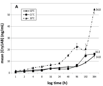
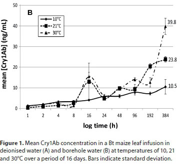
A sample was considered a non-detect (ND) if the optical density value was below that of the blank plus 3 times the standard deviation. The limit of detection (LOD) and limit of quantification (LOQ) were determined using regression analysis of the calibration curves where LOD = 3S_b/b and LOQ = 10S_b/b (S_b = slope uncertainty and b = slope). The LOD was 0.13 ± 0.05 ng/mL and the LOQ was 1.06 ± 0.85 ng/mL.

Statistical analysis

The normality of the data distribution was investigated with the Shapiro-Wilk test to decide on the application of one-way analysis of variance (ANOVA) (if the dataset was normally distributed) or Kruskal-Wallis ANOVA if the dataset was non-normally distributed. IBM's SPSS software package was used for the calculations.

 

RESULTS AND DISCUSSION

There were no detectable levels of Cry proteins in any of the water samples at the start of the experiment before leaf matter was added. The Cry1Ab protein concentration in the control treatments (non-Bt iso-hybrid) was very low with the highest concentration in deionised water and borehole water being 0.13 ng/mL and 0.10 ng/mL, respectively, which were <LOQ (Data not shown). These levels might be ascribed to light absorption in the relevant nanometer range caused by other dissolved compounds that leached out of the plant material or that could also have had an affinity for the antibody on the plates. Nevertheless, these levels were lower than the limit of quantification.

The Cry1Ab concentrations in deionised water and borehole water at the three different temperatures are presented in Figs 1A and 1B, respectively. This study indicated that Cry protein released from Bt maize leaves is more pronounced at higher ambient temperatures. Both infusions at 10°C had lower concentrations of Cry1Ab proteins, varying between 11 and 15 ng/mL up to 16 days after the exposure commenced. Exposure of submerged Bt maize leaves under an ambient temperature of 30^oC resulted in the highest Cry concentration throughout the experiment. The infusions exposed to 30°C had the highest Cry1Ab concentrations after 16 days, ranging between 39.8 ng/mL (borehole water) and 54.8 ng/mL (deionised water), with those exposed at room temperature having concentrations between 16.3 and 23.8 ng/mL (Fig. 1A). For the 10°C treatment, the maximum Cry protein concentrations after 16 days of leaf exposure were 14.8 ng/mL in borehole water and 10.5 ng/mL in deionised water.

The general tendency in all treatments was a slow increase in Cry1Ab concentration over time until the end of the 16-day period. No significant difference in Cry protein concentrations between the two types of water was found. Compared to the two lower temperature treatments, a marked increase in Cry1Ab protein concentration in both water treatments over the latter half of the experiment (192 h onwards) was observed in water kept at 30°C. The concentrations of Cry1Ab protein in the two types of water kept at 30^°C were approximately 3.4- and 1.7-fold higher at the end of the exposure period, compared to the other temperature treatments. It would be expected that the highest concentration of Cry1Ab in the water would be reached later at lower temperatures when compared to higher temperatures. When comparing the entire infusion period, there was a statistically significant difference between Bt protein released into the water at 10°C and 30°C and between 21°C and 30°C, but not between 10°C and 21°C for both the water types (Kruskal-Wallis; p < 0.05). A study by Tank et al. (2010) indicated that the maximum concentration of Cry1Ab protein recorded in natural streams containing maize detritus was 32 ng/L (Tank et al., 2010), much lower than those recorded in this study. Carstens et al. (2012) reported that aquatic organisms in a pond or ditch with maize detritus could be exposed to a maximum concentration of 22.5-1 125 ng/mL or 0.67-33ng/mL of Bt protein, respectively, in the worst-case scenario assumptions for the risk assessment they did. The range of concentrations of Cry proteins recorded after 16 days in the two water types used in this study (Fig. 1A and 1B) ranged between 23.8 and 54.8ng/mL. Comparing this to an approximate 14.7 x 10⁶ µg/mL that could potentially be present in the initial 24 g leaf material (we did not quantify the Cry1Ab contents in the leaf material in this study, but Andreassen et al. (2015) reported 612.51 ng Cry1Ab in 1 mg Mon810 leaf), what seems to be leaching out in these 16 days is but a tiny fraction of the potentially available Cry1Ab. While these concentrations are in the lower range of that predicted by Carstens et al. (2012) for a pond system, they are much higher than that reported by Tank et al. (2010) in natural streams. The methods described in this study can therefore be used as a guideline in planning of risk assessment studies on aquatic organisms, since this study gives an indication of the exposure scenarios that can be developed using these methods.

Strain and Lydy (2015) found that exposure time played a significant role in the release rate of the Cry1Ab proteins into the surrounding environment. They observed that the Cry proteins leached out of the leaf tissues at a rapid rate, peaking within a day or two (depending on the temperature) and then declining. This observation is not supported by our findings, where there was a gradual increase in Cry concentrations after 48 h. Strain and Lydy (2015) also reported higher concentrations of the Bt protein in colder temperatures than warmer temperatures, which is also opposite to the findings we report here. However, the experimental set-up used by Strain and Lydy (2015) was different to ours. The one difference that might explain the decline of Bt proteins from the water in their experiment is the presence of sediment in their microcosm, whereas sediment was absent from our experimental set-up. It is known that Cry proteins strongly adsorb to surface active particles of clay and organic matter in soils (Stotzky, 2005; Mueting et al., 2014), but in the absence of sediment, the Cry protein concentration increased up until the termination of our experiment at the end of Day 16.

The presence of sediment in the Strain and Lydy (2015) microcosm could possibly also explain the higher concentrations reported in the colder water (4°C). In contrast, we report higher concentrations for Cry protein at the higher temperatures and we did not add sediment. The temperatures in the current study were 10°C, 21°C and 30°C, while Strain and Lydy (2015) evaluated the influence of a similar temperature range (4°C, 23°C and 37°C). They added 10 dry leaf disks of 1.8 cm diameter to 75 mL water on top of 5 g sediment, whereas we added strips of dry leaf to the equivalent of 24 g to 1 L of water. Although we cannot definitively compare the leaf mass used in the two experiments, it is clear from the reported levels that the leaf mass:water ratio resulted in two orders of magnitude lower Cry concentrations in this study compared to that reported by Strain and Lydy (2015). Both Strain and Lydy (2015) and this study made use of unsterilised water (and unsterilised sediment in the case of Strain and Lydy (2015)), and although they reported no significant difference between the Cry levels in the unsterilised and sterilised aquatic environments, we postulate that the soil bacteria in the sediment could have metabolised the Cry proteins (Valldor et al., 2015). Furthermore, at higher temperatures higher metabolic rates may lead to decreased Cry protein levels. Because the present study was conducted without sediment, it is likely that there would have been less bacterial activity in our experimental set-up, explaining the steady increase in Cry levels over time. The plant material would also degrade quicker at higher temperatures, releasing the Cry protein and, in the absence of adsorbing sediment, contributing to the higher Cry levels at higher temperatures in this study.

No studies that can inform risk assessments regarding the effect of Bt maize on aquatic ecosystems have been done in South Africa. It is important that future studies address the possible effects of Cry proteins on non-target species that are closely related to the target pests of Cry proteins. Although the target Lepidoptera species of the Cry1Ab protein are all crop pests, off-target effects on other lepidopteran species may result if susceptible and closely related species ingest such proteins. Although Lepidoptera are characteristically terrestrial, the Pyralidae family includes several species with truly aquatic larvae (Gerber and Gabriel, 2002). The Pyralidae family also includes several maize and sugarcane pests which are susceptible to Cry1Ab protein, for example, Eldana saccharina (Walker) (Keeping et al. 2007) and Chilo partellus (Swinhoe) in South Africa (Van Rensburg, 1999).

 

CONCLUSIONS

Our data showed that accumulation of Cry1Ab protein released by Bt maize leaves is influenced by temperature and that the concentration of Cry proteins may increase over time. This study also quantified levels of Cry protein present in water that contains Bt maize leaf tissue in the absence of confounding factors such as sediment (and its associated microbial activity). These factors should be considered during risk assessment studies with aquatic organisms. The characterization of exposure of aquatic organisms along with the known specificity of the insecticidal trait, linked to the ecology of non-target species present in that habitat (in particular those closely related to Lepidoptera or other target groups), will contribute to improved risk assessment studies on aquatic environments.

 

AUTHOR CONTRIBUTIONS

Amy du Pisanie performed all experimental and analytical procedures, and prepared the first draft of the manuscript for submission. LH. du Preez and J van den Berg were supervisors of the study and R Pieters assisted with the ELISA and writing of the manuscript.

 

SOURCES OF FUNDING

This study was funded by Biosafety South Africa (Project BS08-001) and we accordingly give due acknowledgment.

 

CONFLICTS OF INTEREST

The authors have no conflicts of interest to declare.

 

REFERENCES

ANDREASSEN M, BØHN T, WIKMARK O-G, VAN DEN BERG J, LØVIK M, TRAAVIK T and NYGAARD UC (2015) Cry1Ab protein from Bacillus thuringiensis and MON810 cry1Ab-transgenic maize exerts no adjuvant effect after airway exposure. Scand. J. Immunol. 81 192-200 https://doi.org/10.1111/sji.12269        [ Links ]

BAUMGARTE S and TEBBE CC (2005) Field studies on the environmental fate of Cry1Ab Bt-toxin produced by transgenic maize (MON810) and its effect on bacterial communities in the maize rhizosphere. Molec. Ecol. 14 2539-2551. https://doi.org/10.1111/j.1365-294X.2005.02592.x        [ Links ]

BETZ FS, HAMMOND BG and FUCHS RL (2000) Safety and advantages of Bacillus thuringiensis - Protected plants to control insect pests. Regul. Toxicol. Pharmacol. 32 56-173. https://doi.org/10.1006/rtph.2000.1426        [ Links ]

BØHN T, PRIMICERIO R, HESSEN DO and TRAAVIK T (2008) Reduced fitness of Daphnia magna fed a Bt-transgenic maize variety. Arch. Environ. Contam. Toxicol. 55 584-592. https://doi.org/10.1007/s00244-008-9150-5        [ Links ]

BÖTTGER R, SCHALLER J, LINTOW S and DUDEL EG (2015) Aquatic degradation of Cry1Ab protein and decomposition dynamics of transgenic corn leaves under controlled conditions. Ecotox. Environ. Saf. 113 454-459. https://doi.org/10.1016/j.ecoenv.2014.12.034        [ Links ]

BRAVO A, GILL SS and SOBERóN M (2007) Mode of action of Bacillus thuringiensis Cry and Cyt toxins and their potential for insect control. Toxicon 49 423-435. https://doi.org/10.1016/j.toxicon.2006.11.022        [ Links ]

BRODERICK NA, RAFFA KF and HANDELSMAN J (2006) Midgut bacteria required for Bacillus thuringiensis insecticidal activity. PNAS 103 15196-15199. https://doi.org/10.1073/pnas.0604865103        [ Links ]

BROOKES G and BARFOOT P (2014) Economic impact of GM crops. GM Crops Food 5 65-75. https://doi.org/10.4161/gmcr.28098        [ Links ]

CARSTENS K, ANDERSON J, BACHMAN P, DE SCHRIJVER A, DIVELY G, FEDERICI B, HAMER M, GIELKENS M, JENSEN P, LAMP W, RAUSCHEN S, RIDLEY G, ROMEIS J. and WAGGONER A (2012) Genetically modified crops and aquatic ecosystems: considerations for environmental risk assessment. Transgenic Res. 21 813-842. https://doi.org/10.1007/s11248-011-9569-8        [ Links ]

CHAMBERS CP, WHILES MR, ROSI-MARSHALL EJ, TANK JL, ROYER TV, GRIFFITHS NA, EVANS-WHITE MA and STOJAK AR (2010) Responses of stream macro invertebrates to Bt maize leaf debris. Ecol. Applic. 20 1949-1960. https://doi.org/10.1890/09-0598.1        [ Links ]

FENG Y, LING L, FAN H, LIU Y, TAN F, SHU Y and WANG J (2011) Effects of temperature, water content and pH on degradation of Cry1Ab protein released from Bt corn straw in soil. Soil Biol. Biochem. 43 1600-1606. https://doi.org/10.1016/j.soilbio.2011.04.011        [ Links ]

GERBER A and GABRIEL MJM (2002) Aquatic Invertebrates of South African Rivers. Field Guide. Institute for Water Quality Studies, Department of Water Affairs and Forestry, Pretoria.         [ Links ]

HOLDERBAUM DF, CUHRA M, WICKSON F, ORTH AI, NODARI RO and BØHN T (2015) Chronic responses of Daphnia magna under dietary exposure to leaves of transgenic (event MON810) Bt-maize hybrid and its conventional near isoline. J. Toxicol. Environ. Health A 78 (15) 998-1007. https://doi.org/10.1080/15287394.2015.1037877        [ Links ]

ISAAA (2017) Global Status of Commercialized Biotech/GM Crops: 2017. ISAAA Brief No. 53. ISAAA: Ithaca, New York.         [ Links ]

JENSEN PD, DIVELY GP, SWAN CM and LAMP WO (2010) Exposure and non-target effects of transgenic Bt corn debris in streams. Environ. Entomol. 39 707-714. https://doi.org/10.1603/EN09037        [ Links ]

KEEPING MG, RUTHERFORD RS AND CONLONG DE (2007) Bt-maize as a potential trap crop for management of Eldana saccharina Walker (Lep., Pyralidae) in sugarcane. Appl. Entomol. 131 241-250. https://doi.org/10.1111/j.1439-0418.2007.01147.x        [ Links ]

KRATZ W, MANTE C, HOFMANN F, SHLECHTRIEMEN U, KUHN U, OBER S. and VÖGELD R (2010) Exposure of maize harvest by-products to aquatic ecosystems and protected nature reserves in Brandenburg, Germany. In: Breckling B and Verhoeven R (eds) Implications of GM-Crop Cultivation at Large Spatial Scales. Peter Lang, Frankfurt, Germany. 21-23.         [ Links ]

KRUGER M, VAN RENSBURG JBJ and VAN DEN BERG J (2009) Perspective on the development of stem borer resistance to Bt maize and refuge compliance at the Vaalharts irrigation scheme in South Africa. Crop Protect. 28 684-689. https://doi.org/10.1016/j.cropro.2009.04.001        [ Links ]

LI Y-L, DU J, FANG Z-X and YOU J (2013) Dissipation of insecticidal Cry1Ac protein and its toxicity to nontarget aquatic organisms. J. Agric. Food. Chem. 61 10864-10871. https://doi.org/10.1021/jf403472j        [ Links ]

LI Y, WU K, ZHANG Y and YUAN G (2007) Degradation of Cry1Ac protein within transgenic Bacillus thuringiensis rice tissues under field and laboratory conditions. Environ. Entomol. 36 1275-1282. https://doi.org/10.1093/ee/36.5.1275        [ Links ]

LöVEI GL and ARPAIA S (2005). The impact of transgenic plants on natural enemies: a critical review of laboratory studies. Entomol. Exp. Applic. 114 1-14. https://doi.org/10.1111/j.0013-8703.2005.00235.x        [ Links ]

MASEHELA TS, TERRAPON H, WINKER H and MAPHISA D (2016) An assessment of land use patterns for genetically modified crops in South Africa 2016: Technical Report Volume 1: GMO Monitoring and Research. Report Number: SANBI/GMO2016/2016/Vol1/A. South African National Biodiversity Institute, Newlands, Cape Town.         [ Links ]

MUETING SA, STRAIN KE and LYDY MJ (2014) Validation of an extraction method for Cry1Ab protein from soil. Environ. Toxicol. Chem. 33 18-25. https://doi.org/10.1002/etc.2383        [ Links ]

NARANJO SE (2009) Impacts of Bt crops on non-target invertebrates and insecticide use patterns. CAB Reviews: Perspectives in Agriculture, Veterinary Science, Nutrition and Natural Resources 4, No. 011.         [ Links ]

PALM CJ, DONEGAN K, HARRIS D and SEIDLER RJ (1994) Quantification in soil of Bacillus thuringiensis var. kurstaki δ‐endotoxin from transgenic plants. Molec. Ecol. 3 145-151. https://doi.org/10.1111/j.1365-294X.1994.tb00115.x        [ Links ]

PHILLIPS AM (2008) Cry34Ab1, Cry35Ab1, Cry1F and PAT protein levels in hybrid maize TC1507, DAS-59122-7, MON 89034 x TC1507 x MON 88017 x DAS-59122-7, and a conventional control from the Monsanto 2006 production plan 06-01-52-04, Dow AgroSciences. LLC Sub-Report ID: 061026.05 https://www.testbiotech.org/sites/default/files/SmartStax_Expression_data_Testbiotech.pdf        [ Links ]

PRIHODA KR and COATS JR (2008) Aquatic fate and effects of Bacillus thuringiensis Cry3Bb1 protein: Toward risk assessment. Environ. Toxicol. Chem. 27 793-798. https://doi.org/10.1897/07-300.1        [ Links ]

RAYBOULD A and QUEMADA H (2010) Bt crops and food security in developing countries: realised benefits, sustainable use and lowering barriers to adoption. Food Secur. 2 247-259. https://doi.org/10.1007/s12571-010-0066-3        [ Links ]

ROSI-MARSHALL EJ, TANK JL, ROYER T, WHILES MR, EVANS-WHITE M, CHAMBERS C, GRIFFITHS NA, POKELSEK J and STEPHEN ML (2007) Toxins in transgenic crop by products may affect headwater stream ecosystems. PNAS 104 16204-16208. https://doi.org/10.1073/pnas.0707177104        [ Links ]

SAXENA D, FLORES S and STOTZKY G (1999) Transgenic plants: Insecticidal toxin in root exudates from Bt corn. Nature 402 (6761) 480. https://doi.org/10.1038/44997        [ Links ]

SHOGREN AJ, TANK JL, ROSI EJ, DEE MM, SPEIR SL, BOLSTER D and EGAN SP (2019) Transport and instream removal of the Cry1Ab protein from genetically engineered maize is mediated by biofilms in experimental streams. PLOSONE 14 (5) e0213481.         [ Links ]

STILLWELL L and SILVANOVICH A (2008) Assessment of Cry1A.105, Cry2Ab2, Cry3Bb1, and CP4 EPSPS 59122-7 protein levels in the combined trait corn product MON 89034 × TC1507 × MON 88017 × DAS- 59122-7 produced in U.S. field trials during 2006. Monsanto Company Biotechnology Regulatory Sciences, MSL0021070. URL: https://www.testbiotech.org/sites/default/files/SmartStax_Expression_data_Testbiotech.pdf (Accessed 21 May 2017).         [ Links ]

STOTZKY G (2005) Persistence and biological activity in soil of the insecticidal proteins form Bacillus thuringiensis, especially from transgenic plants. Plant Soil 266 77-89. https://doi.org/10.1007/s11104-005-5945-6        [ Links ]

STRAIN KE, WHITING SA and LYDY MJ (2014) Laboratory and field validation of a Cry1Ab protein quantitation method for water. Talanta 128 109-116. https://doi.org/10.1016/j.talanta.2014.04.036        [ Links ]

STRAIN KE and LYDY MJ (2015) The fate and transport of the Cry1Ab protein in an agricultural field and laboratory aquatic microcosms. Chemosphere 132 94-100. https://doi.org/10.1016/j.chemosphere.2015.03.005        [ Links ]

SWAN CM, JENSEN PD, DIVELY GP and LAMP WO (2009) Processing of transgenic crop residues in stream ecosystem. J. Appl. Ecol. 46 1304-1313. https://doi.org/10.1111/j.1365-2664.2009.01728.x        [ Links ]

TANK JL, ROSI-MARSHALL EJ, ROYERC TV, WHILES MR, GRIFFITHS NA, FRAUENDORF TC and TREERING DJ (2010) Occurrence of maize detritus and a transgenic insecticidal protein (Cry1ab) within the stream network of an agricultural landscape. PNAS 107 17645-17650. https://doi.org/10.1073/pnas.1006925107        [ Links ]

VALLDOR P, MIETHLING-GRAFF R, MARTENS R and TEBBE C (2015) Fate of the insecticidal Cry1Ab protein of GM crops in two agricultural soils as revealed by ¹⁴C-tracer studies. Appl. Microbiol. Biotechnol. 99 7333-7341. https://doi.org/10.1007/s00253-015-6655-5        [ Links ]

VAN DEN BERG J, HILBECK H and BØHN T (2013) Pest resistance to Cry1Ab Bt maize: field resistance, contributing factors and lessons from South Africa. Crop Protect. 54 154-160. https://doi.org/10.1016/j.cropro.2013.08.010        [ Links ]

VAN DEN BERG J and VAN WYK A (2007) The effect of Bt maize on Sesamia calamistis in South Africa. Entomol. Exp. Applic. 122 45-51. https://doi.org/10.1111/j.1570-7458.2006.00492.x        [ Links ]

VAN RENSBURG JBJ (1999) Evaluation of Bt.-transgenic maize for resistance to the stem borers Busseola fusca (Fuller) and Chilo partellus (Swinhoe) in South Africa. S. Afr. J. Plant Soil. 16 38-43.         [ Links ]

VENTER H and BØHN T (2016) Interactions between Bt crops and aquatic ecosystems: a review. Environ. Toxicol. Chem. 35 2891-2902. https://doi.org/10.1002/etc.3583        [ Links ]

VICTOROV AG (2011) Transfer of Bt corn byproducts from terrestrial to stream ecosystems. Russ. J. Plant Phys. 58 543-548. https://doi.org/10.1134/S1021443711040224        [ Links ]

WHITING SA, STRAIN KE, CAMPBEL LA, YOUNG BG and LYDY MJ (2014) A multi-year field study to evaluate the environmental fate and agronomic effects of insecticide mixtures. Sci. Total Environ. 498 543-542. https://doi.org/10.1016/j.scitotenv.2014.07.115        [ Links ]

ZWAHLEN C, HILBECK A, GUGERLI P and NENTWIG W (2003). Degradation of the Cry1Ab protein within transgenic Bacillus thuringiensis corn tissue in the field. Molec. Ecol. 12 765-775. https://doi.org/10.1046/j.1365-294X.2003.01767.x        [ Links ]

 

 

Received 22 May 2018
Accepted in revised form 20 September 2019

 

 

* Corresponding author, email: rialet.pieters@nwu.ac.za

^rND^sANDREASSEN^nM^rND^sBØHN^nT^rND^sWIKMARK^nO-G^rND^sVAN DEN BERG^nJ^rND^sLØVIK^nM^rND^sTRAAVIK^nT^rND^sNYGAARD^nUC^rND^sBAUMGARTE^nS^rND^sTEBBE^nCC^rND^sBETZ^nFS^rND^sHAMMOND^nBG^rND^sFUCHS^nRL^rND^sBØHN^nT^rND^sPRIMICERIO^nR^rND^sHESSEN^nDO^rND^sTRAAVIK^nT^rND^sBÖTTGER^nR^rND^sSCHALLER^nJ^rND^sLINTOW^nS^rND^sDUDEL^nEG^rND^sBRAVO^nA^rND^sGILL^nSS^rND^sSOBERóN^nM^rND^sBRODERICK^nNA^rND^sRAFFA^nKF^rND^sHANDELSMAN^nJ^rND^sBROOKES^nG^rND^sBARFOOT^nP^rND^sCARSTENS^nK^rND^sANDERSON^nJ^rND^sBACHMAN^nP^rND^sDE SCHRIJVER^nA^rND^sDIVELY^nG^rND^sFEDERICI^nB^rND^sHAMER^nM^rND^sGIELKENS^nM^rND^sJENSEN^nP^rND^sLAMP^nW^rND^sRAUSCHEN^nS^rND^sRIDLEY^nG^rND^sROMEIS^nJ^rND^sWAGGONER^nA^rND^sCHAMBERS^nCP^rND^sWHILES^nMR^rND^sROSI-MARSHALL^nEJ^rND^sTANK^nJL^rND^sROYER^nTV^rND^sGRIFFITHS^nNA^rND^sEVANS-WHITE^nMA^rND^sSTOJAK^nAR^rND^sFENG^nY^rND^sLING^nL^rND^sFAN^nH^rND^sLIU^nY^rND^sTAN^nF^rND^sSHU^nY^rND^sWANG^nJ^rND^sHOLDERBAUM^nDF^rND^sCUHRA^nM^rND^sWICKSON^nF^rND^sORTH^nAI^rND^sNODARI^nRO^rND^sBØHN^nT^rND^sJENSEN^nPD^rND^sDIVELY^nGP^rND^sSWAN^nCM^rND^sLAMP^nWO^rND^sKEEPING^nMG^rND^sRUTHERFORD^nRS^rND^sCONLONG^nDE^rND^sKRATZ^nW^rND^sMANTE^nC^rND^sHOFMANN^nF^rND^sSHLECHTRIEMEN^nU^rND^sKUHN^nU^rND^sOBER^nS^rND^sVÖGELD^nR^rND^sKRUGER^nM^rND^sVAN RENSBURG^nJBJ^rND^sVAN DEN BERG^nJ^rND^sLI^nY-L^rND^sDU^nJ^rND^sFANG^nZ-X^rND^sYOU^nJ^rND^sLI^nY^rND^sWU^nK^rND^sZHANG^nY^rND^sYUAN^nG^rND^sLöVEI^nGL^rND^sARPAIA^nS^rND^sMUETING^nSA^rND^sSTRAIN^nKE^rND^sLYDY^nMJ^rND^sPALM^nCJ^rND^sDONEGAN^nK^rND^sHARRIS^nD^rND^sSEIDLER^nRJ^rND^sPRIHODA^nKR^rND^sCOATS^nJR^rND^sRAYBOULD^nA^rND^sQUEMADA^nH^rND^sROSI-MARSHALL^nEJ^rND^sTANK^nJL^rND^sROYER^nT^rND^sWHILES^nMR^rND^sEVANS-WHITE^nM^rND^sCHAMBERS^nC^rND^sGRIFFITHS^nNA^rND^sPOKELSEK^nJ^rND^sSTEPHEN^nML^rND^sSAXENA^nD^rND^sFLORES^nS^rND^sSTOTZKY^nG^rND^sSHOGREN^nAJ^rND^sTANK^nJL^rND^sROSI^nEJ^rND^sDEE^nMM^rND^sSPEIR^nSL^rND^sBOLSTER^nD^rND^sEGAN^nSP^rND^sSTOTZKY^nG^rND^sSTRAIN^nKE^rND^sWHITING^nSA^rND^sLYDY^nMJ^rND^sSTRAIN^nKE^rND^sLYDY^nMJ^rND^sSWAN^nCM^rND^sJENSEN^nPD^rND^sDIVELY^nGP^rND^sLAMP^nWO^rND^sTANK^nJL^rND^sROSI-MARSHALL^nEJ^rND^sROYERC^nTV^rND^sWHILES^nMR^rND^sGRIFFITHS^nNA^rND^sFRAUENDORF^nTC^rND^sTREERING^nDJ^rND^sVALLDOR^nP^rND^sMIETHLING-GRAFF^nR^rND^sMARTENS^nR^rND^sTEBBE^nC^rND^sVAN DEN BERG^nJ^rND^sHILBECK^nH^rND^sBØHN^nT^rND^sVAN DEN BERG^nJ^rND^sVAN WYK^nA^rND^sVAN RENSBURG^nJBJ^rND^sVENTER^nH^rND^sBØHN^nT^rND^sVICTOROV^nAG^rND^sWHITING^nSA^rND^sSTRAIN^nKE^rND^sCAMPBEL^nLA^rND^sYOUNG^nBG^rND^sLYDY^nMJ^rND^sZWAHLEN^nC^rND^sHILBECK^nA^rND^sGUGERLI^nP^rND^sNENTWIG^nW^rND^1A01^nM^sMachete^rND^1A02^nJM^sShadung^rND^1A01^nM^sMachete^rND^1A02^nJM^sShadung^rND^1A01^nM^sMachete^rND^1A02^nJM^sShadung

SHORT COMMUNICATION

 

Detection of selected agricultural pesticides in river and tap water in Letsitele, Lomati and Vals-Renoster catchments, South Africa

 

 

M Machete^{I, *}; JM Shadung^II

^ICollege of Agriculture and Environmental Sciences, University of South Africa (UNISA), Science Campus, Florida Park, South Africa
^IICouncil for Scientific and Industrial Research (CSIR), Natural Resources & the Environment, PO Box 395, Pretoria, 0001, South Africa

 

 

---

ABSTRACT

This paper presents the levels of detection of selected agricultural pesticides in river and tap water in the Letsitele, Lomati and Vals-Renoster catchments, South Africa. Agriculture plays a major role in the development of communities through job creation and poverty eradication. However, exposure to agricultural pesticides can result in serious human health and environmental effects. This study, therefore, identified critical areas where specific pesticides might result in high environmental and human health risks. Three water catchment areas, namely, Letsitele, Lomati and Vals-Renoster, were identified for raw and tap water analysis. The results confirmed the presence of selected agricultural pesticides: atrazine, terbuthylazine, imidacloprid, metolachlor, simazine and alachlor. Although low concentrations of most of these pesticides were detected, pesticides such as atrazine, alachlor and simazine are known for endocrine disruption. A critical finding of this study is the detection of these pesticides in tap water (drinking water) of a primary school in the Lomati catchment. This reveals a high exposure potential for human health. It is thus recommended that further research be conducted to determine the potential health risks associated with these pesticides among vulnerable communities, through epidemiological studies.

Keywords: pesticides, endocrine disruptors, environmental health risks, agriculture, water quality

---

 

 

INTRODUCTION

South Africa has the largest agricultural pesticide market in the sub-Saharan Africa region (Naidoo and Buckley, 2003). The South African National Department of Agriculture, Forestry and Fisheries (DAFF, 2010; 2013) registered a variety of pesticides for agricultural use during the years 2010 and 2013. Dabrowski (2015a) confirmed that more than 3 000 pesticides were registered for use by the agricultural sector in South Africa in 2015. Pesticides are one of the many technologies commonly used to improve agricultural production in South Africa (Dabrowski, 2015a). In an earlier study, Maharaj (2005) raised concern about the increasing trend of pesticide use in South African agricultural production and the number of pesticides used. The primary concern of Maharaj (2005) was the deterioration in the chemical water quality of South Africa's rivers.

Agriculture is one of the key sectors of the South African economy that is relied upon for addressing the country's 26.6% and 39% unemployment and poverty rates, respectively (StatsSA, 2016). In the light of the current levels of unemployment, poverty and inequality, cessation of pesticide use is not considered an option. In contrast to the economic potential of rapid growth of the agricultural sector, the use of most agricultural pesticides presents both chronic and acute environmental and human health risks, particularly for farming communities that are vulnerable due to living in close proximity to pesticide use.

Machete (2017) points out that organic and inorganic elements or compounds of agricultural pesticides are capable of moving from a point of application into non-target environments, particularly in surface and groundwater resources. In an earlier study, Dabrowski and De Klerk (2013) found the presence of agricultural pesticides in the water resources bordering intensely farmed areas, and detected pesticides in ground, surface and drinking water. Various studies have highlighted the persistent nature, mobility and potential environmental risks associated with a number of commonly used agricultural pesticides (Schulz, 2001; Footprint, 2006; Dabrowski, 2015a; Machete, 2017).

Numerous chronic and acute environmental health risks are associated with agricultural pesticide exposure. Footprint (2006) and Schulz (2001) concur that environmental exposure to agricultural pesticides is responsible for many incidences of toxicity to aquatic organisms. For instance, chlorpyrifos and endosulfan have been detected in environmental water samples at levels that may be toxic to fish and other macro-invertebrates (Dabrowski et al., 2014). According to Hallenbeck and Cunningham-Burns (2011), agricultural pesticides contain chemical elements or compounds that are carcinogenic, teratogenic, mutagenic and endocrine disruptive to living organisms (including human beings).

In developing countries, the use of agricultural pesticides has been associated with a myriad of detrimental effects on female health (London et al., 2002). In South Africa, the consequence of pesticide exposure has been related to several human health effects such as endocrine disruption, among others (Aneck-Hahn et al., 2007; English et al., 2012). In light of the seriousness of the environmental health risks associated with agricultural pesticide exposure, this study aimed to determine if agricultural pesticides could be detected in river and tap water in Letsitele, Lomati and Vals-Renoster catchments, South Africa.

 

MATERIALS AND METHODS

This study was conducted in three farmed water catchment areas, namely, Letsitele, Lomati, and Vals-Renoster. The three catchment areas were selected due to suspected potentially high pesticide contamination.

Letsitele catchment

The Letsitele River is located in Limpopo. The river drains the Wolkberg Mountains and flows in a north-easterly direction towards the town, Letsitele, where it flows into the Letaba River. The upper reaches of the catchment mainly comprise of commercial forestry. The river passes through intensively cultivated commercial agricultural land where avocados, citrus fruit and mangoes are produced. Human settlements with domestic livestock and communal gardens occur in close proximity to these commercial agricultural areas. The towns of Khujwana and Mogoboya are adjacent to the Letsitele River near fruit orchards. The upper sections of the catchment are characterised by relatively steep slopes, resulting in a relatively high runoff potential for pesticides. The main soil type is a sandy clay loam, which has a relatively high percentage of sand and is thus susceptible to leaching agrochemicals (Dabrowski, 2015a). This study identified these fruit orchards as potential sources for pesticide spray drift towards human settlements and water sources. Thus, the catchment area and specific sites in it were selected for the purposes of tracing potential endocrine-disrupting chemicals (EDCs) in the domestic water supply.

Lomati catchment

The Lomati River is located in the eastern part of Mpumalanga, north of Eswatini and south of Mozambique. Sugarcane production is the primary agricultural activity undertaken in the surrounding areas, with a smaller proportion contributed by maize, mangoes, bananas and wheat production. The Lomati River originates in Eswatini and flows into Driekoppies Dam and then into the Komati River. Agricultural activities are generally undertaken on low to medium gradient slopes of relatively sandy soil. The mean annual precipitation for the Lomati catchment is 880 mm (Deksissa et al., 2003), with most rainfall occurring in the summer months between November and March.

Vals and Renoster catchments

The Vals River flows in a westerly direction from upstream of Kroonstad past Khotsong and Bothaville before entering the Vaal River. Kroonstad is located midway along the river between VL3 and VL2 and this section of the river is affected by a number of industries and point-source pollution impacts (e.g. sewage outfalls). The catchment of the Renoster River is also an intensive agricultural area, and few large towns are situated along the length of the river. The river flows northwards, entering the Vaal River upstream of its confluence with the Vals River. Relatively few large towns are located along the length of the river (Dabrowski, 2015b). Agricultural activity in the Vals and Renoster catchments consists of intensive maize production along with sorghum and sunflower production. The catchment area is predominately agricultural and is particularly flat in the lower reaches. It has a high proportion of sandy soils which are associated with increased pesticide leaching potential (Dabrowski, 2015b).

Sampling

A total of 14 water sampling points were selected across the three catchments (Table 1).

Three samples were collected from Letsitele, five from Lomati and six from Vals−Renoster (see Table 1). Four seasonal sampling sessions were conducted for each sampling point.

Selection of pesticides for analysis

Information on pesticide use per crop at a national scale (DAFF, 2013) was used to prioritise specific pesticides for testing and analysis in the 14 samples collected. Quarterly raw and tap water samples were collected and analysed to assess the presence of pesticides and their seasonal variation, if any. All raw water samples were collected in 1 L amber glass bottles at approximately 50 cm below the water surface for raw water sampling. All raw and tap water samples were transported on ice at 4°C until delivered to an accredited laboratory. The pesticide crop prioritisation matrix identifies atrazine, terbuthylazine, imidacloprid, metolachlor, simazine and alachlor as relatively high national priority pesticides used in agriculture. Atrazine, alachlor and simazine are among the 12 known endocrine disrupting pesticides (Footprint, 2006; McKinlay et al., 2008).

Quantitative analysis of GC-MS

Liquid-to-liquid extraction was used to extract samples, which involved collecting the organic layer; adjusting the pH; shaking and filtering. The elution was rotary evaporated to the required final volume of 0.5 mL and analysed on capillary column GC-MSD for organophosphates (following the method of Dabrowski et al., 2014).

 

RESULTS AND DISCUSSION

Letsitele catchment

Five EDC pesticides were present at the Letsitele catchment sites (1) upstream (LT3), (2) tap at a public primary school (LT4) and (3) downstream (LT9), as presented in Fig. 1.

The results show a high detection level of diphenylamine, imazalil, thiabendazole, imidacloprid and propiconazole in November 2011. Much higher concentrations of imazalil, thiabendazole and diphenylamine were observed, with propiconazole and imidacloprid occurring at lower concentrations. EDCs were detected in the tap water (drinking water) from a borehole at a primary school in Letsitele Furthermore, a much higher concentration of diphenylamine, imizalil and thiabendazole was detected in November 2011, with propiconazole consistently detected in the tap water at the primary school in almost all seasons, with the exception of the August and November 2012 sampling seasons. The results also show higher EDC concentration in ground water than in surface water, as seen for LT3 and LT4 samples across seasons. Consistent detection of higher levels of imidacloprid at LT9 in all seasons were also noted, as compared to its absence in LT3.

Lomati catchment

Based on the type of agricultural production and potential EDC pesticides used in the catchment area, the concentrations (μg/L) of selected pesticides were analysed in water samples collected from selected sites in the Lomati catchment area (Fig. 2).

The results show no detected EDCs in the June 2012 sampling season. However, during the September and December 2012 and March 2013 sampling seasons, atrazine, imidacloprid, terbuthylazine and carbofuran were detected at varying concentrations. Atrazine was detected in all samples, despite being at low concentrations. It was noted that atrazine concentration was at higher levels in NK4 during September and December 2012 than for all other sampling sites. All the above-mentioned five pesticides were detected at NK3, NK3-tap, NK4 and NK6 sampling sites. Higher concentrations of pesticides were consistently detected at NK4 throughout the sampling period when compared to the other sites. It is also noted that NK5 was the least contaminated of all sites. However, the presence of EDCs in the NK3 tap water is of serious concern, as it represents direct human exposure to the pesticides, in particular schoolchildren in the school where the tap is located and is used for drinking water supply.

Vals-Renoster water catchment

Presence and concentrations of atrazine, alachlor, imadaclopid and terbuthylazine (μg/L) were analysed in water samples collected from selected sites in the Vals and Renoster catchments, based on the prevailing agricultural production practices and types of pesticides used (Fig. 3).

The results confirm the presence of atrazine, alachlor, imadaclopid and terbuthylazine in different samples in all seasons in the Vals and Renoster catchments. Although not all samples had all five EDCs detected in equal frequencies and concentrations, all EDCs were detected at one or more sampling sites during each sampling season. In January and April 2013 (rainy season), the concentration levels showed an increase for atrazine, simazine and terbuthylazine. The samples from VL2 and VL3 showed consistently high concentrations of simazine, atrazine and terbuthylazine in January and April 2013, followed by RN3 in January 2013 and VL3 in April 2013. The detection and concentrations indicate a relationship between the rainy season and leaching of EDC pesticides, as found in previous studies (Schulz, 2001; Dabrowski and Schulz, 2003; Dabrowski, 2015b).

 

CONCLUSION

This study confirmed traces of various EDC pesticides in raw and drinking water in the Letsitele, Lomati and Vals-Renoster catchment areas. Traces of pesticides in borehole and reticulated tap water samples were confirmed in Nkomati and Letsitele, respectively. The pesticides investigated are known EDCs, and were found at high concentrations in some instances. Wu et al. (2009) found that exposure to atrazine concentrations as low as 0.1 ppb can alter the sex characteristics of male frogs, resulting in male frogs with female sex characteristics, hermaphroditism and the presence of eggs in male frog testes. The current study found much higher concentrations of atrazine and other EDCs in drinking water in this study, which presents a much higher potential of exposure and the possibility of a myriad of effects on humans and the environment (fauna and flora). The (ATSDR, 2003), found that atrazine can cause liver, kidney and heart damage in animals, and could possibly cause cancer in humans. Maternal exposure to atrazine has been associated with low birth weights, heart, urinary and limb defects in humans. Wu et al. (2009) report that atrazine exposure can lead to adverse reproductive effects in animals and humans, even at low levels of exposure. When exposure coincides with the development of the brain and reproductive organs, the effects may be even more severe. Also of great concern is the potential for atrazine to act synergistically with other pesticides to increase their toxic effects. Fitzmayer et al. (1982) and Garry (2004) confirmed the acute toxicity effects of simazine and other EDCs on human health, particularly in children. Further studies are recommended, including epidemiological investigations to establish the prevalence of environmental health risks and specifically to establish a cause-effect relationship between human exposure to the studied pesticides and potential environmental health risks highlighted in other studies. Finally, this study also highlights the question of the efficacy of existing water treatment technologies in the study areas, due to their inability to completely eliminate EDCs during water treatment processes. This suggests the need for water treatment in the indicated areas to be investigated.

 

ACKNOWLEDGEMENTS

This paper has emerged from a research project funded by the Water Research Commission (Report No. 1956/1/15), the Council for Scientific and Industrial Research (CSIR), under the Natural Resources and the Environment Business Unit. Data analysis, presentation of results, write-up and editing of this paper was sponsored by Ga-Machete Guesthouses.

 

REFERENCES

ATSDR (Agency for Toxic Substances and Disease Registry) (2003) Public Health Statement for Atrazine. URL: https://www.atsdr.cdc.gov/phs/phs.asp?id=336&tid=59. (Accessed 5 June 2017).         [ Links ]

ANECK-HAHN, NH, SCHULENBURG GW, BORNMAN MS, FARIAS P and DE JAGER C (2007) Impaired semen quality associated with environmental DDT exposure in young men living in a malaria area in the Limpopo Province, South Africa. J. Androl. 28 (3) 423-434. https://doi.org/10.2164/jandrol.106.001701        [ Links ]

DABROWSKI JM (2015a) Development of pesticide use maps for South Africa. S. Afr. J. Sci. 111 (1-2) 07. https://doi.org/10.17159/sajs.2015/20140091        [ Links ]

DABROWSKI JM (2015b) Investigation of the contamination of water resources by agricultural chemicals and the impact on environmental health. Volume 1: Risk assessment of agricultural chemicals to human and animal health. WRC Report No. 1956/1/15.         [ Links ]

DABROWSKI JM and DE KLERK LP (2013) An assessment of the impact of different land use activities on water quality in the upper Olifants River catchment. Water SA 39 (2) 231-244. https://doi.org/10.4314/wsa.v39i2.6        [ Links ]

DABROWSKI JM and SCHULZ R (2003) Predicted and measured levels of azinphosmethyl in the Lourens River, South Africa. Comparison of runoff and spray drift. Environ. Toxic. Chem. 22 (3) 494-500. https://doi.org/10.1002/etc.5620220305        [ Links ]

DABROWSKI JM, SHADUNG MJ and WEPENER V (2014) Prioritizing agricultural pesticides used in South Africa based on their environmental mobility and potential human health effects. Environ. Int. 62 31-40. https://doi.org/10.1016/j.envint.2013.10.001        [ Links ]

DAFF (Department of Agriculture, Forestry and Fisheries, South Africa) (2010) Pesticide management policy for South Africa. Government Gazette No. 33899, Pretoria.         [ Links ]

DAFF (Department of Agriculture, Forestry and Fisheries, South Africa) (2013) Trends in the agricultural sector. DAFF, Pretoria.         [ Links ]

DEKSISSA T, ASHTON PJ and VANROLLEGHEM (2003) Control options for river water quality improvement: A case study of TDS and inorganic nitrogen in the Crocodile River (South Africa). Water SA 29 (209) 217. https://doi.org/10.4314/wsa.v29i2.4858        [ Links ]

ENGLISH RG, PERRY M, LEE MM, HOFFMAN E, DELPORT S and DALVIE MA (2012) Farm residence and reproductive health among young boys in rural South Africa. Environ. Int. 47 73-79. https://doi.org/10.1016/j.envint.2012.06.006        [ Links ]

FITZMAYER KM, GEIGER JG and VAN-DEN-AVYLE MJ (1982) Acute toxicity effects of simazine on Daphnia pulex and larval striped bass. Proceedings of the thirty sixth annual conference. S.E. Assoc of Fish and Wildlife Agen. 36 146-156.         [ Links ]

FOOTPRINT (2006) Footprint Pesticide Properties Database. Database collated by the University of Hertfordshire as part of the EU-funded Footprint project (FP6-SSP-022704).URL: http://www.eu-footprint.org/ppdb.html (Accessed 7 April 2010).         [ Links ]

GARRY VV (2004) Pesticides and children. Toxic. Appl. Pharmacol. 198 (2) 152-163. https://doi.org/10.1016/j.taap.2003.11.027        [ Links ]

HALLENBECK WH and CUNNINGHAM-BURNS KM (2011) Pesticides and Human Health. Springer, London. 166 pp.         [ Links ]

LONDON L, DE GROSBOIS S, WESSELING C, KISTING S, ROTHER HA and MERGLER D (2002) Pesticides usage and health consequences for women in developing countries: Out of sight, out of mind? Int. J. Occup. Environ. Health 8 46-59. https://doi.org/10.1179/oeh.2002.8.1.46        [ Links ]

MACHETE F (2017) Environmental health risks associated with e-waste exposure in Badplaas, Carolina and Elukwatini landfills, Republic of South Africa. Afr. J. Sci. Technol. Innov. Dev. 9 (7) 679-684. https://doi.org/10.1080/20421338.2017.1355602        [ Links ]

MAHARAJ S (2005) Modelling the behaviour and fate of priority pesticides in South Africa. MSc. dissertation, University of the Western Cape.         [ Links ]

MCKINLAY R, PLANT JA, BELL JNB and VOULVOULIS N (2008). Endocrine disrupting pesticides: implications for risk assessment. Environ. Int. 34 168-183. https://doi.org/10.1016/j.envint.2007.07.013        [ Links ]

NAIDOO V and BUCKLEY CA (2003) Survey of pesticide wastes in South Africa and review of treatment options. WRC Report No. 1128/1/03, Water Research Commission, Pretoria.         [ Links ]

SCHULZ R (2001) Rainfall-induced sediment and pesticide input from orchards into the Lourens River, Western Cape, South Africa: importance of a single event. Water Res. 35 1869-1876. https://doi.org/10.1016/S0043-1354(00)00458-9        [ Links ]

STATS SA (Statistics South Africa) (2016) Community Survey 2016: Statistics release, P0301. URL: http://cs2016.statssa.gov.za/wp-content/uploads/2016/07/NT-30-06-2016-RELEASE-for-CS-2016-_Statistical-releas_1-July-2016.pdf (Accessed 8 August 2016).         [ Links ]

 

 

Received 15 June 2017
Accepted in revised form 4 October 2019

 

 

* Corresponding author, email: mtec.dr@gmail.com

^rND^sANECK-HAHN^nNH^rND^sSCHULENBURG^nGW^rND^sBORNMAN^nMS^rND^sFARIAS^nP^rND^sDE JAGER^nC^rND^sDABROWSKI^nJM^rND^sDABROWSKI^nJM^rND^sDE KLERK^nLP^rND^sDABROWSKI^nJM^rND^sSCHULZ^nR^rND^sDABROWSKI^nJM^rND^sSHADUNG^nMJ^rND^sWEPENER^nV^rND^sDEKSISSA^nT^rND^sASHTON^nPJ^rND^sVANROLLEGHEM^rND^sENGLISH^nRG^rND^sPERRY^nM^rND^sLEE^nMM^rND^sHOFFMAN^nE^rND^sDELPORT^nS^rND^sDALVIE^nMA^rND^sFITZMAYER^nKM^rND^sGEIGER^nJG^rND^sVAN-DEN-AVYLE^nMJ^rND^sGARRY^nVV^rND^sLONDON^nL^rND^sDE GROSBOIS^nS^rND^sWESSELING^nC^rND^sKISTING^nS^rND^sROTHER^nHA^rND^sMERGLER^nD^rND^sMACHETE^nF^rND^sMCKINLAY^nR^rND^sPLANT^nJA^rND^sBELL^nJNB^rND^sVOULVOULIS^nN^rND^sSCHULZ^nR^rND^1A01 A03^nBeaven^sUtete^rND^1A02^nCrispen^sPhiri^rND^1A03^nTosan B^sFregene^rND^1A01 A03^nBeaven^sUtete^rND^1A02^nCrispen^sPhiri^rND^1A03^nTosan B^sFregene^rND^1A01 A03^nBeaven^sUtete^rND^1A02^nCrispen^sPhiri^rND^1A03^nTosan B^sFregene

RESEARCH PAPERS

 

Drivers and barriers to sustainable fisheries in two peri-urban impoundments in Zimbabwe

 

 

Beaven Utete^{I, III, *}; Crispen Phiri^II; Tosan B Fregene^III

^IDepartment of Wildlife Ecology and Conservation, Chinhoyi University of Technology, Chinhoyi, Zimbabwe
^IIDepartment of Freshwater and Fishery Science, Chinhoyi University of Technology, Chinhoyi, Zimbabwe
^IIIDepartment of Aquaculture and Fisheries Management, University of Ibadan, Oyo State, Nigeria

 

 

---

ABSTRACT

Fisheries sustainability is categorised through four conceptual pillars: ecological, economic, and social, including cultural and institutional. Much work on fisheries sustainability has been done in marine fisheries relative to inland fisheries. Two inland peri-urban impoundments, Chivero and Manyame in Zimbabwe, support numerous small-scale fisheries; however, environmental and socioeconomic variables threaten the sustainability of the fisheries. This study aimed to identify and contextualise drivers and barriers to sustainability of small-scale fisheries in these two peri-urban impoundments. We applied three frameworks, Fishery Performance Indicators, Community-Based Fishery Indicators and FAO Small-Scale Fisheries Indicators, to identify and contextualise the drivers and barriers. Quantitative and qualitative methods were used to collect data from fishers in the two impoundments. A structured questionnaire was administered to 115 fishers in 23 fishing companies operating in the two lakes. Fisheries income and revenue as well as food security are key drivers. Lack of post-harvest equipment, volatile fish markets, water quality and quantity deterioration and fish stock decreases are key barriers to sustainability of fisheries in the two impoundments. There are subtle differences in the extent and impact of the drivers and barriers of fisheries sustainability in the two lakes. The differences relate to the uniqueness of the aquatic habitats, social constructs and fisheries operational frameworks in each lake. This suggests a need to assess fisheries sustainability using an integrated bottom-up approach starting from individual fisheries < community fisheries < global/generic fisheries.

Keywords: peri-urban fisheries, food security, water resource conservation, water pollution, sustainability

---

 

 

INTRODUCTION

Small-scale inland fisheries provide essential ecosystem services comprising food, nutrient cycling in water, employment and income to millions of people, and generate foreign currency for developing countries such as Zimbabwe in Sub-Saharan Africa (Allison et al., 2009; Marshall, 2011; FAO, 2013, 2014a,b,c, 2016; Bartley et al., 2015). Inland fisheries support numerous livelihoods and enhance the socio-economic development of urban and rural areas in Africa (Allan, 2005; WorldFish, 2009; AU-IBAR, 2012; De Graaf and Garibaldi, 2014). However, the sustainability of inland fisheries is threatened by a plethora of factors, including aquatic environmental degradation (Welcomme et al., 2009; Cooke et al., 2012), overexploitation and overfishing (FAO, 2015; 2016) and market volatility of fish prices (Taylor et al., 2007; Vörösmarty et al., 2010). The dynamics in other factors such as geographical expansion, fishing capacity-building, natural variability and climate change further threaten the viability of inland fisheries (Béné, 2003; Allison and Horemans, 2006; Garcia and Rosenberg, 2010). Hence it is imperative to effectively monitor and assess the state of freshwater inland fisheries (FAO, 2016).

Within Africa, contemporary fisheries assessment and management remain heavily dominated by the ecological aspects and to a lesser extent the economic aspects (Stephenson et al., 2018). No comprehensive and holistic frameworks exist to integrate and evaluate various other aspects such as the cultural, political, institutional and social elements threatening the sustainability of small-scale inland capture fisheries (Bond and Morrison-Saunders, 2011; FAO, 2016; Thompson and Stephenson, 2016). The challenge in evaluating the sustainability of fisheries is largely driven by a lack of reliable and consistent fisheries statistics (Cooke et al., 2013), and non-cogent classification of small-scale fisheries into urban, rural and peri-urban sets, and this tends to complicate effective management of small-scale inland fisheries (Béné et al., 2003; Kebe and Tallec, 2006; FAO, 2010; Bartley et al., 2015). As a result of lack of a clear assessment framework for sustainability and reliable statistics, small-scale inland fisheries are excluded from national and regional economic planning initiatives and are notably absent in the Sustainable Development Goals (Bartley et al., 2015, FAO, 2015; Link et al., 2017; Stephenson et al., 2018). Clearly, there is a need for a framework that assesses the ecological, economic, institutional and social elements or indicators of fisheries to evaluate their sustainability (Stephenson et al., 2018).

Two contiguous peri-urban eutrophic lakes, Chivero and Manyame, in Zimbabwe support numerous fisheries and provide vital ecosystems services such as potable water and habitat for aquatic organisms (Marshall, 2011). The viability and sustainability of the fisheries in the two impoundments is threatened by a number of factors such as water pollution, climate change, over-abstraction of the water and competing water withdrawing activities (Magadza, 2011; Mhlanga and Mhlanga, 2013). Despite their ecological and socioeconomic significance, fisheries in urban and peri-urban impoundments such as Chivero and Manyame are not often a national priority and are undervalued and largely overlooked in Zimbabwe (FAO, 2015; Kupaza et al., 2015). This study aimed to identify and contextualise drivers and barriers to sustainability of small-scale fisheries in these two peri-urban impoundments. Three indicators - Fishery Performance Indicators (FPI) described by Anderson et al. (2015), Community-Based Fishery Indicators (CFI) following Boyd and Charles (2006) and FAO Small-Scale Fisheries Indicators (FSSFI) (FAO, 2015) - shown in Table 1, were used to evaluate the drivers and barriers threatening the sustainability of fisheries and viability of fishing livelihoods in Lakes Chivero and Manyame, Zimbabwe.

 

MATERIAL AND METHODS

Study area

Lakes Chivero and Manyame (Fig. 1) are two peri-urban impoundments located about 30-40 km south-east of Harare, the capital city of Zimbabwe (Magadza, 2003). Morphometrically, Lake Chivero has a capacity of 247 181 × 10⁶ m³, a mean depth of 9.4 m and a surface area of 2 630 ha with a retention time of 1.1 years. Lake Manyame has a surface area of 8 100 ha at full capacity, when its maximum and mean depths are 23 m and 5.6 m, respectively, with an estimated mean retention time of 0.7 years (Marshall, 2011; Utete et al., 2018). The impoundments were constructed in 1952 and 1976, respectively, to mainly provide potable water to Harare (then Salisbury City). However, other uses such as water abstraction for irrigation, small-scale and subsistence fishing and recreational activities such as boating, angling and birdwatching have evolved over the years (Marshall, 2011).

With regard to small-scale fishing, there are a total of 23 fishing cooperatives (12 in Lake Chivero and 11 in Lake Manyame). Each fishing cooperative consists of at least 8-11 members who contribute fishing gear (boats and nets), labour and start-up capital, as well as paying the permit fees to National Parks (Utete et al., 2018). The fisheries from Lake Chivero have been estimated to catch an annual yield of 250 kg∙h^-1∙yr^-1 fish (Marshall, 2011), though there is no clear estimate of catches in Lake Manyame (Utete et al., 2018). The allowed mesh sizes in the two lakes range from 26 mm to 152 mm (1-6'') with 12.5 mm (0.5'') increments (Marshall, 2011). Fish catches have been declining in the two lakes, thus threatening the sustainability of the fisheries and the livelihoods of the fishers (Utete et al., 2018). Hence there is a need for an integrated framework to assess the sustainability of the fisheries, not only from a stock assessment perspective but using a holistic lens approach encompassing other covariates such as water pollution, post-harvest considerations, market accessibility as well as demographic aspects (FAO, 2015).

Data collection

We employed a mix of quantitative and qualitative methods to collect data from fishers in 2017. A structured questionnaire was administered to 115 fishers in 23 fishing cooperatives operating in Lakes Chivero and Manyame. Focus group discussions and key informant interviews were done on active men and women fishers, and Parks officials responsible for Lakes Chivero and Manyame, in order to have an in-depth qualitative cross-validation of the drivers and challenges affecting their livelihoods. From 115 questionnaires administered, 87 fully completed ones were used for further data analysis.

Description of the indicator frameworks and their assessment in fisheries

Three indicators, Fishery Performance Indicators (FPI) after Anderson et al. (2015), Community-Based Fishery Indicators (CFI) by Boyd and Charles (2006) and FAO Small-Scale Fisheries Indicators (FSSFI) frameworks, summarised in Table 1, were used to evaluate the drivers and barriers threatening the sustainability of fisheries and viability of fishing livelihoods in Lakes Chivero and Manyame, Zimbabwe. Conceptually, separating measures of performance, the FPI uses 68 individual outcome metrics - coded on a 1 to 5 scale based on expert assessment to facilitate application to data-poor fisheries and sectors - that can be partitioned into sector-based or triple-bottom-line sustainability-based interpretative indicators conveniently classified into ecology, economic, social and community aspects (Anderson et al., 2015). For any given fishery or cooperative, the respondents, who were mostly fishers, were asked a raft of closed and open-ended questions which are broadly classified into ecology, economic, social and institutional aspects. Every recurring theme or response is scored on a scale of 1 to 5 and the results are collated as a mean for each theme in the main classification scheme. The frequency of recurrence of any theme implies its significance as an aspect to measure the sustainability of the fishery (Chu et al., 2017).

The Community-Based Fishery Indicators (CFI) by Boyd and Charles (2006) presupposes a collection of fisheries in a water body to be a fishing community. Then it assesses a wide array of aspects ranging from the fishing fleets or vessels, nets, gender composition and roles, access to financial capital, fishery training facilities and opportunities afforded to the fishing community. It also assesses on a thematic basis the perceptions of the fishing community on fish stocks, depletion levels, and environmental issues such as water pollution and climate change (Boyd and Charles, 2006). Frequently recurring or generic issues across the fishing community are broadly categorised into ecological, social, economic and institutional categories (Boyd and Charles, 2006; FAO, 2015). The idea is not to weigh the significance of the factors but to get a holistic perspective from the fishing communities who are on the ground on the topical or recurring factors affecting their viability and livelihoods (FAO, 2015). This enables broad policy considerations rather than narrow quantified (weighed) aspects which tend to shift over temporal scales in fishing communities as the aquatic environment is largely dynamic (Bartley et al., 2015).

The FAO Small-Scale Fisheries Indicators (FSSFI) target mainly small-scale fishers who are considered as self-employed (FAO, 2013). The main factors considered are the food security and nutrition levels of the fishers, largely driven by fish stock dynamics, water quality concerns, climate change, changes in fishing regulations, fish poaching and competition for fishing zones (FAO, 2015). FSSI tends to evaluate the ecological elements of the fishing business on a Likert scale of 1-4 or 1-5, based on the mean responses or perceptions of the fishers themselves. In line with other fishery indicators, the most recurrent themes for any given fishery are allocated high scores 4 or 5 on the scale and are the key factors to be considered in fisheries management and ensuring and evaluating sustainability of small-scale inland fisheries (Stephenson et al., 2018).

Comparative analysis of the perceptions of fishers

After identification of the most recurrent factors influencing sustainability of small-scale fisheries in the two lakes using the three indicator frameworks, we further comparatively tested for the significance of differences in the perceptions of fishers in Lakes Chivero and Manyame towards the types of drivers and barriers affecting their livelihoods. For clarity, the mean perceptions are derived from the Likert Scale of: 1 = strongly disagree, 2 = disagree, 3 = agree, and 4 = strongly agree. Fishers in the two lakes were used as the test groups. After testing for normality using the Kolmogorov-Smirnov test, the data were found to be non-parametric, and thus we used descriptive and multivariate inferential statistics. We treated the two lakes as categorical groups, and since our perceptions were on a Likert scale of 1-4 we applied the 2-way contingency Chi square (χ²) test of homogeneity for comparison at the 5% level using the SPSS 21 version. The same test was also used to assess for differences in the livelihood strategies of the respondents between the two lakes.

 

RESULTS

Demography and livelihood strategies of fishers in the two impoundments

The basic demography of the fisheries in Lakes Chivero (males = 34, females = 1) and Manyame (males = 45, female = 7) was skewed towards males. The majority (n = 13; 37%) of the fishers were primarily involved in fishing and farming, and the rest (n = 8; 23%) were fish traders in Lake Chivero (Table 2). In Lake Manyame, the majority (n = 32; 62%) of the fishers were directly and actively involved in fishing, whereas a sizeable portion (n = 10; 19%) of the fishers were also into fish marketing and 10% (n = 5) were engaged in trading and repairing of fishing gear such as nets and boats. The rest of the respondents (n = 5; 10%) were into farming as an alternative livelihood strategy in Lake Manyame (Table 2). Statistical analysis indicated a significant difference (χ² (3) = 14.749; p < 0.05) in the actual livelihood strategies between the two lakes. For Lake Manyame, the hierarchy for the livelihood strategies was: fishing > trading > farming > others, whilst for Lake Chivero it was: farming > fishing > trading > others.

 

 

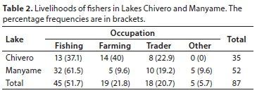
Drivers and barriers of fisheries sustainability in Lakes Chivero and Manyame based on the fisheries viability indicator frameworks

From the three indicator frameworks applied for the Lakes Chivero and Manyame, the FPI framework identified ecological elements such as depleting fish catches/stocks, deteriorating water quality, dynamic land-use patterns and climate change as barriers threatening the sustainability of the fisheries. Economic barriers such as volatile markets, poor post-harvest preservation infrastructure, expensive annual fishing permits and unskilled fish processing workers also threaten sustainability of small-scale fisheries in both lakes. Social factors such as rapid fisheries managerial and casual labour turnovers, as well as lack of cross linkages with communities and unguaranteed short-term fisheries careers, act as barriers to the viability and sustainability of fisheries in the two lakes. Institutional or governance issues such as inaccessible fishing and harvesting rights are barriers to the sustainability of fisheries and livelihoods of fishers in Lakes Chivero and Manyame in Zimbabwe. Lack of collective bargaining action, for instance towards accessing loans and capital to maintain fisheries viability, is a barrier to sustainability of the fisheries. Inadequate participation of the community and exclusion of females in fisheries governance is a barrier to the sustainability of fisheries in the two lakes as indicated by the FPI (Table 3).

The CFI framework identified reductions in fish biodiversity, deterioration in the quality of lake habitat, decreases in fishable areas and drawdown zones as well as reductions in the catch of targeted species and an increase in by-catch wastes as ecological barriers to the sustainability of fishing communities in Lakes Chivero and Manyame. Fluctuations in the income value of fish harvests/catches, low market incentives for fisheries and fish which tend to be seasonal, as well as the low credit worthiness and natural capital are economic barriers to fishing-dependent communities in both lakes (Table 3). Dynamics in the demographic structure of fishing communities as well as access to fishing-related education and contribution and cooperation of marginal groups such as females and youths are some of the social factors affecting the two fishing communities (Table 3). Lack of an integrated approach towards research and management of fisheries resources are barriers towards sustainability of fishing communities (Table 3).

Using the FSSFI framework, aquatic habitat pollution and degradation are the main ecological barriers for sustainability of fisheries in the two lakes (Table 3). Volatile income from fish sales is the main economic barrier for sustainability of the small-scale fisheries in Lakes Chivero and Manyame (Table 3). Failure to uphold or respect cultures and ensuring gender equality and equity are social barriers for sustainable small-scale fisheries in the FSSFI framework (Table 2). Within the governance and institutional elements, lack of transparency of fisheries management, effective implementation of fishing rules and unclear access regulations are key barriers for sustainable fisheries in Lakes Chivero and Manyame (Table 3).

An evaluative summary of the three fisheries indicators show that fisheries-related income, employment, level of education of the fishers, and guaranteed food security and nutrition from fisheries, as well as accessible fish markets, are the key drivers for the sustainability of small-scale inland fisheries in the two lakes. Other key driving factors for sustainable fisheries comprise the level of fishing technology, such as fishing gear, boats and suitable post-harvest facilities, available (Table 3).

Demography and comparative analysis of perceptions of fishers in the two impoundments

The basic demography of the fisheries in Lakes Chivero (males = 34, females = 1) and Manyame (males = 45, female = 7) was skewed towards males with a large proportion 91% (n = 79) and the rest 9% (n = 8) were females.

The drivers and barriers facing small-scale inland fisheries suggested by peri-urban fishers and as indicated by the three frameworks were added and the results are summarised in Table 4. Among the identified drivers in sustainability of fisheries there were significant differences (χ² (3), p < 0.05 in the educational levels towards fishing-related issues among fishers in Lakes Chivero and Manyame (Table 4). There is a significant difference (χ² (3), p < 0.05) in the importance of fish harvest incomes as a driver for fishing among fishers between the two lakes. There is a significant difference (χ² (3), p < 0.05) in the fishers' perceptions towards the benefit of fish catches and by-catch wastes for food security between the two lakes (Table 4). Fishers in both lakes do not differ (χ² (3),p > 0.05) in their perceptions towards the availability and dynamics of the fish market as a driver of sustainability of fisheries (Table 4).

 

 

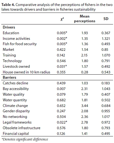
Fishers in Lakes Chivero and Manyame concur (χ² (3),p > 0.05) that declines in peri-urban fish stocks, reductions in water quality and quantity as well as climate change, gender disproportion, poor networking among fishers, and obsolete post-harvest equipment and infrastructure, as well as inaccessible and low financial capital, are the main barriers to sustainability of fisheries (Table 4). Most fishers in both lakes consider bay accessibility / fishing zone restrictions / prohibitions as barriers for their fishing business. However, fishers from both lakes differ significantly in their perceptions of the barrier role played by reduced fishing bay accessibility on fish catches (χ²(3), p < 0.05) and the lack of legal frameworks (χ²(3), p < 0.05) in the sustainability of fisheries in the two lakes (Table 4).

 

DISCUSSION

The main aim of the study was to identify and contextualise drivers and barriers to sustainability of small-scale fisheries in two peri-urban impoundments Chivero and Manyame in Zimbabwe. Three indicators: Fishery Performance Indicator (FPI), Community-Based Fishery Indicators (CFI) and FAO Small-Scale Fisheries Indicator (FSSFI) frameworks were used to evaluate the drivers and barriers affecting the sustainability of fisheries, and viability of fishing-dependent livelihoods in the two lakes.

Results of the study indicated the need for a consistent income, food security, and food nutrition as the main drivers of small-scale inland fisheries in Lakes Chivero and Manyame. Accessible fish markets and the educational levels of the fishers are also key drivers for the sustainability of small-scale inland fisheries in the two lakes. These findings resonate with research by Allison and Ellis (2001); Béné (2003) and FAO (2015), which reflect that small-scale inland fisheries serve multiple purposes, although food security, food nutrition and an income to alleviate poverty form the main basis for continued operations. The educational levels of fishers are key drivers of fisheries sustainability as they infer a capacity to: undergo fisheries and water resource conservation training, adopt new fishing methods and adapt to new post-harvest technologies (Fregene, 2002).

The three fisheries indicator assessment frameworks revealed almost similar ecological, economic, social and institutional barriers to the sustainability of the peri-urban fisheries in Lakes Chivero and Manyame. The FPI, in particular, indicated ecological barriers such as depleting fish stocks, water pollution, climate change and dynamics in land use patterns in the catchment as the main barriers to the sustainability of small-scale fisheries. The CFI indicated similar results with the FPI as it identified declines in targeted fish stocks and biodiversity as the key barriers to the sustainability of small-scale fisheries. The FSSFI indicated aquatic environmental degradation and practice of unsustainable fishing methods as the key ecological barriers to the sustainability of fisheries in Lakes Chivero and Manyame. The ecological barriers identified in this study resonate with generic ecological hazards threatening the sustainability of most marine, coastal and inland fisheries. Béné (2003); Béné et al. (2009); Allison et al. (2005, 2009); Marshall (2011); Kolding and Van Zwieten (2012); FAO (2012, 2016) largely attribute key ecological elements such as unfishable drawdown zones, depleting fish stocks and poor water quality and erratic water level fluctuations as barriers to the sustainability of inland fisheries in Benin, Chad, Cameroon, Zimbabwe, Niger and Malawi. For this study, the deteriorating water quality standards, declining fish stocks and biodiversity in the two peri-urban impoundments are owed to the transboundary (complex mixture of urban and rural characteristics) nature of the catchment areas, punctuated by a lack of clear demarcation and improper water and land resource governance (Nhapi and Gijzen, 2004; Khan et al., 2013).

The three indicator frameworks reflected economic barriers, such as poor post-harvest infrastructure, low recapitalisation and creditworthiness, volatile fish markets and subdued seasonal prices, as key threats to the sustainability of the fisheries in both lakes. Seasonal fluctuations in fish stocks tend to affect the fish prices at the fish markets in the two lakes, with prices relatively higher in the winter season (Seijo et al., 1998; FAO, 2015; Mhlanga and Mhlanga, 2013; Kupaza et al., 2015). The lack of efficient and climate-smart fishing and post-harvest technologies in small-scale inland fisheries affects fishing effort, fish catches and the subsequent market prices (Fregene, 2002). This economic barrier leads to price disparities in small-scale inland fisheries which tend to lead fishers to overexploit the fisheries resources using high fishing effort and inefficient gear (Béné, 2003; 2009).

The demographic distribution of the fishers showed male dominance in the two impoundments. All three fisheries assessment frameworks indicated social barriers such as disproportionate gender consideration, where females are marginalised and perform peripheral and fringe post-harvest roles, including fish gutting, gleaning, and cleaning in fisheries. Undefined and peripheral roles for women, even though they may be as educated as men in leadership positions, in the peri-urban fisheries ensures male domination of the industry (Matsue et al., 2014). The peri-urban nature of the two impoundments implies that women and the youths who are equally affected by poverty would have been attracted to fishing as an alternative source of income to alleviate poverty (Nelson et al., 2008; Khan et al., 2013; FAO, 2016). However, the FSSFI framework indicated a strict adherence to cultural values within the fishing communities, where some fisheries do not deliberately employ women for cultural, ethical and inferred hygienic reasons, which are largely mythical as stated by Allison et al. (2009) Béné (2009) and Matsue et al., (2014). This tends to marginalise women from lucrative fishing operations and economically disempowers them and discourages females from considering fishing as a career in both impoundments (Matsue et al., 2014).

From a governance and institutional perspective, the three frameworks showed that barriers such as restricted access to lucrative fishing zones, expensive annual fishing permits, low consideration for fisheries project management and extension services, fishing land access, rules, laws, and regulation awareness, as well as water conservation education and awareness, affect the sustainability of fisheries in both impoundments. Lack of transparency in fisheries operations is a highlighted barrier indicated by the FSSI, threatening the sustainability of small-scale inland fisheries. Lack of training and extension services may hinder adoption and transfer of fishing technologies to peri-urban fisherfolks and threatens the sustainability of individual small-scale inland fisheries (Adelekan and Fregene, 2015). Even more so, the peri-urban fisheries have poor social organisational networks, limited access to financial capital, rely on obsolete equipment and hardly have legal representation, and this threatens their sustainability (Béné, 2009). In most cases, institutional elements of fisheries are neglected and lead to their non-consideration in economic planning and governance processes (Fregene, 2002; Béné, 2009, Welcomme et al., 2010; Bartley et al., 2015; Link et al., 2017; Stephen et al., 2018).

There are subtle differences in the key drivers and barriers reflected by the three indicator frameworks. This is because the three fisheries viability assessment frameworks lack conceptual coherence and often neglect to incorporate important aspects of the fishery system. In fact most fisheries sustainability assessment frameworks tend to consider individual fisheries, and are dimensional with much focus on fish stock assessment (Béné, 2009; Bartley et al., 2015), water and habitat dynamics (Marshall, 2011; Tendaupenyu, 2012, Nyarumbu and Magadza, 2016), impacts on fishing-dependent livelihoods (Garba, 1997; Allison et al., 2005; Salmi, 2005; Mhlanga and Mhlanga, 2013) or currently the effects of climate change (Brander, 2010; Welcomme et al., 2010; FAO, 2012; 2016; Wichelns, 2017). This suggests a need to assess fisheries sustainability using a bottom-up approach starting from individual fisheries < community fisheries < global/generic fisheries (Seijo et al., 1998; FAO, 2012; 2015). Inclusion of cultural, social, governance, ecological and economic aspects will lead to a holistic assessment of the sustainability of fisheries.

Comparative assessment of the perceptions of the fishers in Lakes Chivero and Manyame towards the drivers and barriers to the sustainability of fisheries reveal significant differences in perspectives towards drivers, such as the effect of educational levels, alternative income strategies adopted, food security of fishing livelihoods, and livestock owned. Some fishers consider the individuals' educational level to be irrelevant as a motivational factor driving fishing activities. Rather, fishing is viewed as a physical activity needing minimal cognitive effort. Fregene (2002) argues that such an attitude hinders the smooth operation and uptake of fisheries extension and management training services in most small-scale inland fisheries in Sub-Saharan Africa. Fishers from the two lakes differ significantly (p < 0.05) in their perspectives towards the need to earn an income from fishing being a driver of sustainability of fisheries. Rather, they relate the need to maximise profits with overexploitation and overfishing of the fisheries resources, often using unregulated gear in the two lakes. Thus, fishers in the two lakes tend to use illegal gear in order to maximise catches, resulting in overfishing which in the long-term threatens the sustainability of the fisheries and livelihoods of fishers themselves (see Tweddle et al., 2015; Irvine et al., 2018).

The significant differences in fishers' perceptions towards a need for food security as a driver of fisheries sustainability in the two lakes indicates that fishers have different motivational factors for continuing with fishing as a livelihood strategy. Fishers significantly disagree that owning livestock such as cattle and goats is a driver of fisheries sustainability in the two lakes. This partly reflects the peri-urban nature of the two lakes, and proximity of Lake Chivero to the main capital city of Harare, relative to Lake Manyame. Fishers in Lake Chivero adopt a more urban lifestyle and tend to alternatively go into non-fishing-related income activities such as trinket trading, tobacco marketing and formal jobs (FAO, 2013; Kupaza et al., 2015). Fishers in Lake Manyame adopt a more rural lifestyle with agriculture and livestock ranching as an alternative livelihood. Non-significant differences in perceptions towards most of the barriers to the sustainability of the fisheries between fishers in the two lakes indicated the universal nature of challenges facing small-scale inland fisheries, such as poor water quality and quantity (FAO, 2015), depleting fish stocks (Welcomme et al., 2010; Tweddle et al., 2015), climate change (Brander, 2010), gender disparity (Matsue et al., 2014), low capital and poor post-harvest technology (Fregene, 2002) and peri-urbanisation (Khan et al., 2013; Nagendra and Ostrom, 2014).

 

CONCLUSIONS AND RECOMMENDATIONS

The main drivers for sustainability of fisheries include the need for a consistent income, food security and food nutrition in Lakes Chivero and Manyame. The applied fisheries sustainability assessment indices; the FPI, CFI and FSSFI, indicated similar barriers threatening the viability of the small-scale inland fisheries. However, the significant differences in the perceptions of small-scale inland fishers towards the barriers and drivers of fisheries between the two lakes shows the inherent uniqueness of individual fisheries and fishers. Thus, in order to guarantee the sustainability of the fisheries in the two peri-urban lakes, there is a need to consider a bottom-up approach incorporating the concerns of individual fisheries which then feeds into community fisheries and can inform global fisheries aspects. Even more so, future studies of fisheries may exploit the integrated application of a raft of fisheries assessment frameworks for effective evaluation of their sustainability in the face of ecological, economic, social and institutional threats.

 

ACKNOWLEDGEMENTS

Our special thanks go to Mr Newman Songore at Lake Chivero Fisheries Research Station and all the Parks staff for assistance with the field logistics. We thank the Graduate Studies Office at Chinhoyi University of Technology for funding this research under Grant PG 4299. This research was also supported by funding from the Department for International Development (DFID) under the Climate Impact Research Capacity and Leadership Enhancement (CIRCLE) programme, implemented by the African Academy of Sciences (AAS) and the Association of Commonwealth Universities (ACU). We also thank the two anonymous reviewers who made this manuscript readable.

 

REFERENCES

ADELEKAN I and FREGENE T (2015) Vulnerability of artisanal fishing communities to flood risks in coastal southwest Nigeria. Clim. Dev. 7 (4) 322-338. https://doi.org/10.1080/17565529.2014.951011        [ Links ]

AU-IBAR (African Union InterAfrican Bureau for Animal Resources) (2012) Regional assessment of fisheries issues, challenges and opportunities in Southern African region. Towards the formulation of the policy framework and reform strategy for fisheries and aquaculture in Africa. AU-IBAR, Nairobi.         [ Links ]

ALLISON EH and HOREMANS B (2006) Putting the principles of the sustainable livelihoods approach into fisheries development policy and practice. Mar. Pol. 30 757-766. https://doi.org/10.1016/j.marpol.2006.02.001        [ Links ]

ALLISON E and ELLIS F (2001) The livelihoods approach and management of small-scale fisheries. Mar. Pol. 25 377-388. https://doi.org/10.1016/S0308-597X(01)00023-9        [ Links ]

ALLISON E, ADGER N, BADJECK M, BROWN K, CONWAY D, DULVY N, HALLS A, PERRY A and REYNOLDS J (2005) Effects of climate change on the sustainability of capture and enhancement fisheries important to the poor: analysis of the vulnerability and adaptability of fisherfolk living in poverty. DFID Technical report. Project R4778J. DFID, Marine Resources Assessment Group, London, UK, 169 pp.         [ Links ]

ALLISON EH, PERRY AL, BADJECK MC, ADGER WN, BROWN K, CONWAY D, HALLS AS, PILLING GM, REYNOLDS JD, ANDREW NL and DULVY N (2009) Vulnerability of national economies to the impacts of climate change on fisheries. Fish Fish. 10 173-196. https://doi.org/10.1111/j.1467-2979.2008.00310.x        [ Links ]

ANDERSON JL, ANDERSON CM, CHU J, MERIDETH J, ASCHE F, SYLVIA G and VALDERRAMA D (2015) The fishery performance indicators. A management tool for triple bottom line outcomes, PLoS ONE 10 e0122809. https://doi.org/10.1371/journal.pone.0122809        [ Links ]

BARTLEY DM, de GRAAF GJ, VALBO-JØRGENSEN J and MARMULLA G (2015) Inland capture fisheries: status and data issues. Fish. Manage. Ecol. 22 (1) 71-77. https://doi.org/10.1111/fme.12104        [ Links ]

BÉNÉ C (2003) When fishery rhymes with poverty: a first step beyond the old paradigm on poverty in small-scale fisheries. World Dev. 31 (6) 949-975. https://doi.org/10.1016/S0305-750X(03)00045-7        [ Links ]

BÉNÉ C, NEILAND AE, JOLLEY T, OVIE S, SULE O, LADU B, MINDJIMBA K, BELAL E, TIOTSOP F, BABA M, DARA L, ZAKARA A and QUENSIERE J (2003) Inland fisheries, poverty and rural livelihoods in the Lake Chad Basin. J. As. Afr. Stud. 38 (1) 17-51. https://doi.org/10.1177/002190960303800102        [ Links ]

BÉNÉ C (2009) Are fishers poor or vulnerable? Assessing economic vulnerability in small- scale fishing communities. J. Dev. Stud. 45 (6) 911-933. https://doi.org/10.1080/00220380902807395        [ Links ]

BÉNÉ C, STEEL E, KAMBALA LUADIA B and GORDON A (2009) Fish as the bank in the water-evidence from chronic-poor communities in Congo. Food Policy 34 104-118. https://doi.org/10.1016/j.foodpol.2008.07.001        [ Links ]

BOYD H and CHARLES A (2006) Creating community based indicators to monitor sustainability of local fisheries. Ocean Coast. Manage. 49 237-258. https://doi.org/10.1016/j.ocecoaman.2006.03.006        [ Links ]

BRANDER K (2010) Impacts of climate change on fisheries. J. Mar. Syst. 79 389-402. https://doi.org/10.1016/j.jmarsys.2008.12.015        [ Links ]

CHU J, GARLOCK T, ASCHE F and ANDERSON JL (2017) Impact evaluation of a fisheries development project. Mar. Pol. 85 141-149. https://doi.org/10.1016/j.marpol.2017.08.024        [ Links ]

COOKE SJ, PAUKERT C and HOGAN Z (2012) Endangered river fish: factors hindering conservation and restoration. Endanger. Species Res.17 179-191. https://doi.org/10.3354/esr00426        [ Links ]

COOKE SJ, LAPOINTE NWR, MARTINS EG, THIEM JD, RABY GD, TAYLOR MK, BEARD TDJR and COWX IG (2013) Failure to engage the public in issues related to inland fishes and fisheries: strategies for building public and political will to promote meaningful conservation. J. Fish Biol. 83 (4) 997-1018. https://doi.org/10.1111/jfb.12222        [ Links ]

DE GRAAF G and GARIBALDI L (2014) The value of African fisheries. FAO Fisheries and Aquaculture Circular 1093 76.         [ Links ]

SEIJO JC, DEFEO O and SALAS S (1998) Fisheries bio-economics theory: modelling and management. FAO Fisheries Technical Paper. Food and Agriculture Organization of the United Nations, Rome. 368 pp.         [ Links ]

FAO (2012) The State of World Fisheries and Aquaculture 2012. Food and Agriculture Organisation, Rome. 209 pp.         [ Links ]

FAO (2013) Statistics. Capture production 1950-2011. URL: http://www.fao.org/fishery/statistics/en (Accessed 13 February 2017).         [ Links ]

FAO (2014) The State of World Fisheries and Aquaculture 2014. Food and Agriculture Organisation of the United Nations, Rome. 223 pp.         [ Links ]

FAO (2014a) CWP Handbook of Fishery Statistical Standards. Section G: Fishing Areas - General. Rome, Italy.         [ Links ]

FAO (2014b) The State of World Fisheries and Aquaculture - 2014 (SOFIA). Rome, Italy.         [ Links ]

FAO (2014c) The Water-Energy-Food Nexus: A New Approach in Support of Food Security and Sustainable Agriculture. Food and Agriculture Organisation of the United Nations, Rome.         [ Links ]

FAO (2015) Voluntary guidelines for securing sustainable small-scale fisheries. URL: http://www.fao.org/policy-support/resources/resources-details/en/c/418453/ (Accessed 24 March 2017).         [ Links ]

FAO (2016) The State of World Fisheries and Aquaculture 2016. Food and Agriculture Organisation of the United Nations, Rome. 200 pp.         [ Links ]

FREGENE BT (2002) Poverty assessment of fishing communities of Lagos State, Nigeria. PhD thesis, University of Ibadan, Nigeria.         [ Links ]

GARCIA SM and ROSENBERG AA (2010) Food security and marine capture fisheries: characteristics, trends, drivers and future perspectives. Philos. Trans. R. Soc. B 365 (1554). https://doi.org/10.1098/rstb.2010.0171        [ Links ]

GARBA AR (1997) The importance of nomadic education in Nigeria. New Nigeria September 1997. 16 pp.         [ Links ]

GILLETT R (2009) Fisheries in the Economies of Pacific Island Countries and Territories.: Asian Development Bank, Mandaluyong City, Philippines. 484 pp.         [ Links ]

HOWELLS MS, HERMANN M, WELSCH M, BAZILIAN R, SEGERSTRÖM R, ALFSTAD D, GIELEN H, ROGNER G, FISCHER H, VAN VELTHUIZEN D and co-authors (2013) Integrated analysis of climate change, land-use, energy and water strategies. Nat. Clim. Change 3 621-626. https://doi.org/10.1038/nclimate1789        [ Links ]

KÉBÉ M and TALLEC F (2006) Contribution of fisheries sector to national economies (West and Central Africa). Sustainable Fisheries Livelihoods Programme (SFLP) in West Africa. Impression AGCom, Cotonou, Benin.         [ Links ]

KHAN MSA, PRAKASH A, NARAIN V and SADA R (2013) Adapting to peri-urban water insecurity induced by urbanization and climate change: insights from South Asia. Proceedings of the Resilient Cities 2013 Congress, 31 May-2 June Bonn, Germany.         [ Links ]

KOLDING J and VAN ZWITTEN PAM (2012) Relative lake level fluctuations and their influence on productivity and resilience in tropical lakes and reservoirs. Fish. Res. (115-116) 99-109. https://doi.org/10.1016/j.fishres.2011.11.008        [ Links ]

IRVINE K, ETIEGNI CA and WEYL OLF (2018) Prognosis for long term sustainable fisheries in the African Great Lakes. Fish. Manage. Ecol. 00 1-13. https://doi.org/10.1111/fme.12282        [ Links ]

LINK JS, THÉBAUD O, SMITH DC, SMITH ADM, SCHMIDT J, RICE J, POOS JJ, PITA C, LIPTON D, KRAAN M and co-authors (2017) Keeping humans in the ecosystem. ICES J. Mar. Sci. 74 1947-1956. https://doi.org/10.1093/icesjms/fsx130        [ Links ]

MAGADZA CHD (2003) Lake Chivero: A management case study. Lakes Reserv. Res. Manage. 8 69-81. https://doi.org/10.1046/j.1320-5331.2003.00214.x        [ Links ]

MARSHALL BE (2011) Fishes of Zimbabwe and their Biology. Smithiana Monograph 3. The Southern African Institute for Aquatic Biodiversity, Grahamstown.         [ Links ]

NAGENDRA H and OSTROM E (2014) Applying the social-ecological system framework to the diagnosis of urban lake commons in Bangalore, India. Ecol. Soc. 19 (2) 67-72. https://doi.org/10.5751/ES-06582-190267        [ Links ]

NELSON R, HOWDEN SM and STAFFORD SMITH M (2008) Using adaptive governance to rethink the way science supports Australian drought policy. Environ. Sci. Polic. 11 588-601. https://doi.org/10.1016/j.envsci.2008.06.005        [ Links ]

NHAPI I and GIJZEN HJ (2004) Wastewater management in Zimbabwe in the context of sustainability, Water Polic. J. 6 (6) 115-121. https://doi.org/10.2166/wp.2004.0033        [ Links ]

NHIWATIWA T, BARSON M, HARRISON AP, UTETE B and COOPER RG (2011) Metal concentrations in sharptooth catfish (Clarias gariepinus, Burchell 1822), sediments and water in peri-urban rivers in Zimbabwe. Afr. J. Aquat. Sci. 3 243-252. https://doi.org/10.2989/16085914.2011.636906        [ Links ]

NYARUMBU TO and MAGADZA CHD (2016) Using the Planning and Management Models of Lakes and Reservoirs (PAMOLARE) as a tool for planning the rehabilitation of Lake Chivero, Zimbabwe. Environ. Nano. Monit. Manage. 5 1-12. https://doi.org/10.1016/j.enmm.2015.10.002        [ Links ]

STEPHENSON RL, PAUL S, WIBER M, ANGEL E, BENSON AJ, CHARLES A, CHOUINARD O, CLEMENS M, EDWARDS D, FOLEY P and co-authors (2018) Evaluating and implementing social-ecological systems: A comprehensive approach to sustainable fisheries. Fish Fish. 19 (5) 853-873. https://doi.org/10.1111/faf.12296        [ Links ]

TAYLOR WW, LEONARD NJ, KRATZER JF, GODDARD C and STEWART P (2007) Globalization: implications for fish, fisheries and their management. In: Taylor WW, Schechter MG and Wolfson LG (eds) Globalization: Effects on Fisheries Resources. Cambridge University Press, Cambridge, UK. 21-46 pp. https://doi.org/10.1017/CBO9780511542183.005        [ Links ]

TENDAUPENYU P (2012) Nutrient limitation of phytoplankton in five impoundments on the Manyame River, Zimbabwe. Water SA 38 (1) 97-104. https://doi.org/10.4314/wsa.v38i1.12        [ Links ]

TWEDDLE D, COWX IG, PEEL R and WEYL OLF (2015) Challenges in fisheries management in the Zambezi, one of the great rivers of Africa. Fish. Manage. Ecol. 22 99-111. https://doi.org/10.1111/fme.12107        [ Links ]

UTETE, B, PHIRI C, MLAMBO SS, MUBOKO N and FREGENE BT (2018) Fish catches, and the influence of climatic and non-climatic factors in Lakes Chivero and Manyame, Zimbabwe. Cogent Food Agric. 4 (1) https://doi.org/10.1080/23311932.2018.1435018        [ Links ]

VÖRÖSMARTY CJ, MCINTYRE PB, GESSNER MO, DUDGEON D, PRUSEVICH A, GREEN P and GLIDDEN S (2010) Global threats to human water security and river biodiversity. Nature 467 (7315) 555-561. https://doi.org/10.1038/nature09440        [ Links ]

WELCOMME RL, COWX IG, COATES D, BÉNÉ C, FUNGE-SMITH S, HALLS A and LORENZEN K (2010) Inland capture fisheries. Phil. Trans. of the Royal Soc. of Biol. 365 2881-2896. https://doi.org/10.1098/rstb.2010.0168        [ Links ]

WEPENER W, VAN VUREN JHJ and DU PREEZ HH (2001) Uptake and Distribution of a copper, iron and zinc mixture in gill, live rand plasma of a freshwater teleost, Tilapia sparmanii. Water SA 27 (1) 99-108. https://doi.org/10.4314/wsa.v27i1.5016        [ Links ]

WICHELNS D (2017) The water-energy-food nexus: Is the increasing attention warranted, from either a research or policy perspective? Environ. Sci. & Pol. 69 113-123. https://doi.org/10.1016/j.envsci.2016.12.018        [ Links ]

WorldFish Center (2009) Fish and aquaculture in a changing climate. Proceedings from the UNFCCC COP-15, December 2009, Copenhagen.         [ Links ]

 

 

Received 9 August 2018
Accepted in revised form 26 September 2019

 

 

* Corresponding author, email: mkaiyo@gmail.com
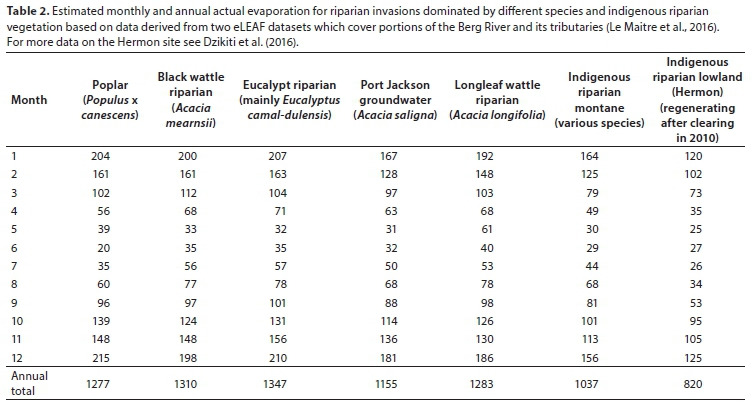
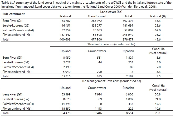
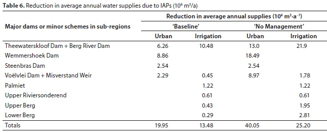
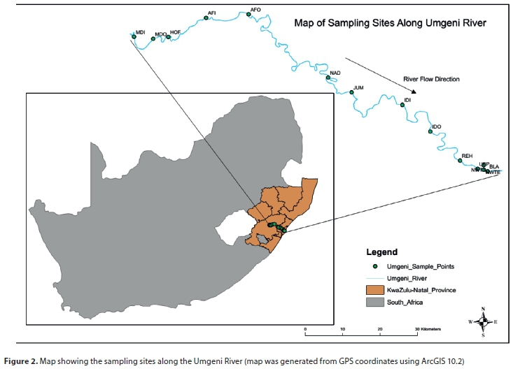
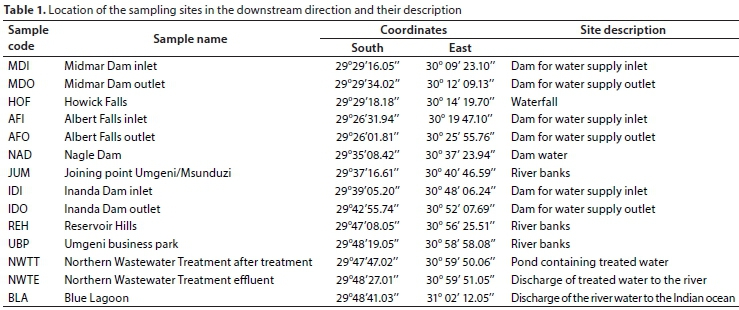
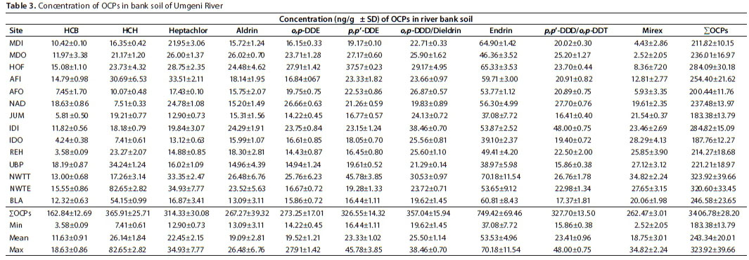
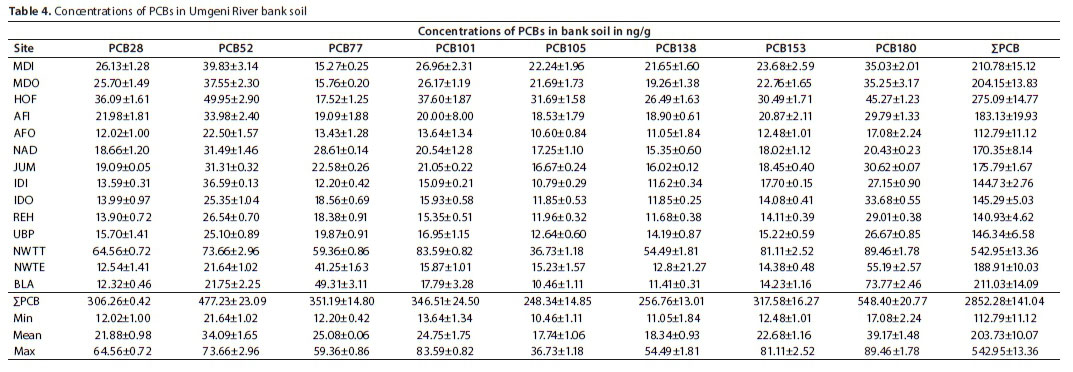
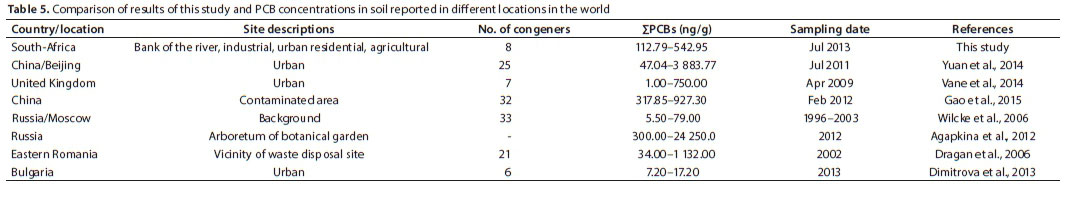
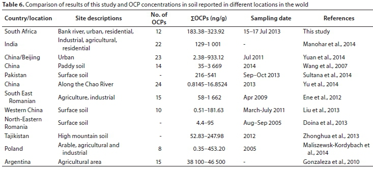
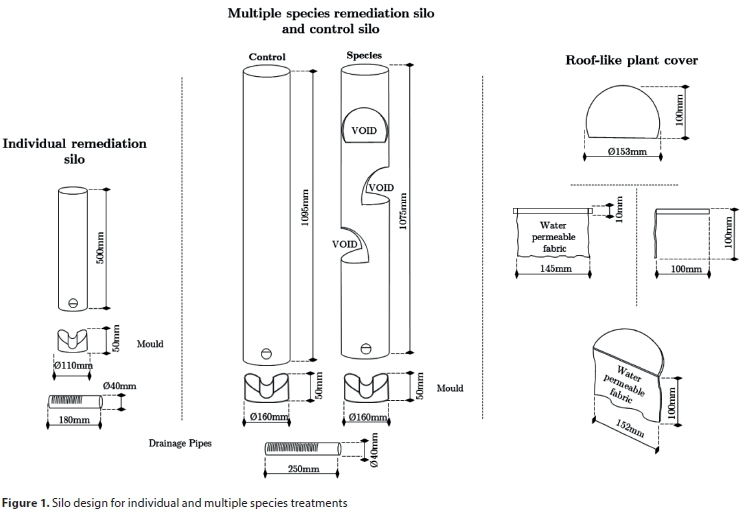
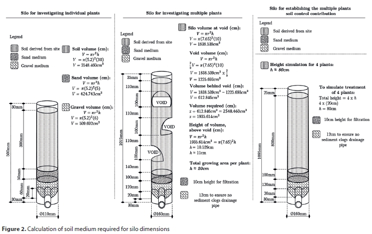
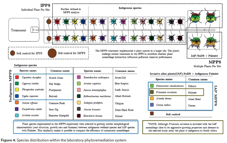
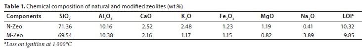
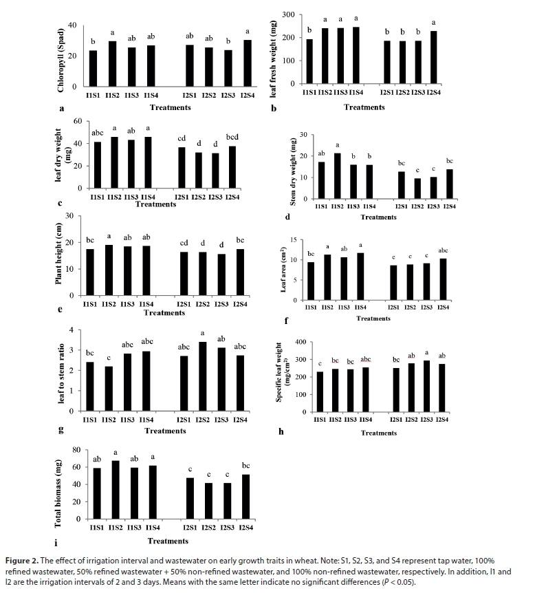
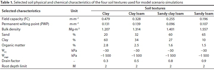
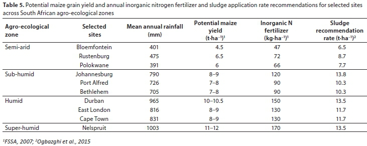
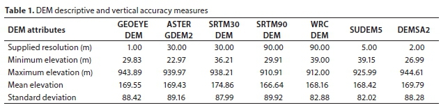
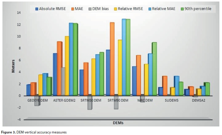
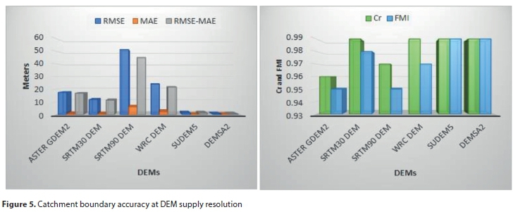
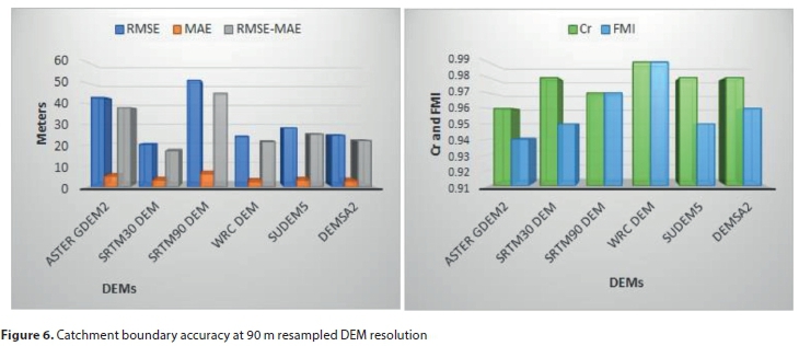
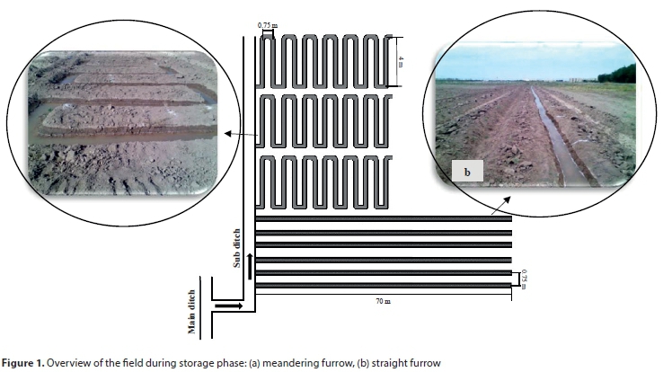
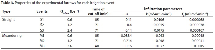
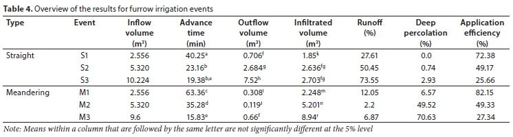
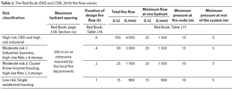
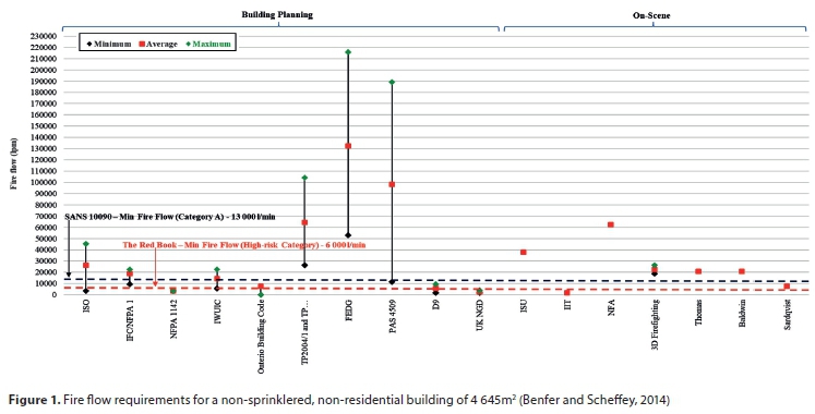
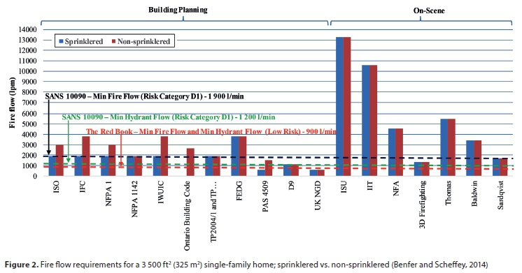
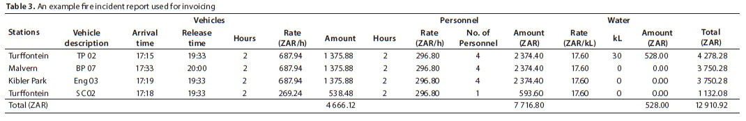
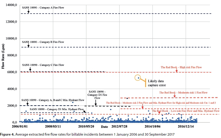
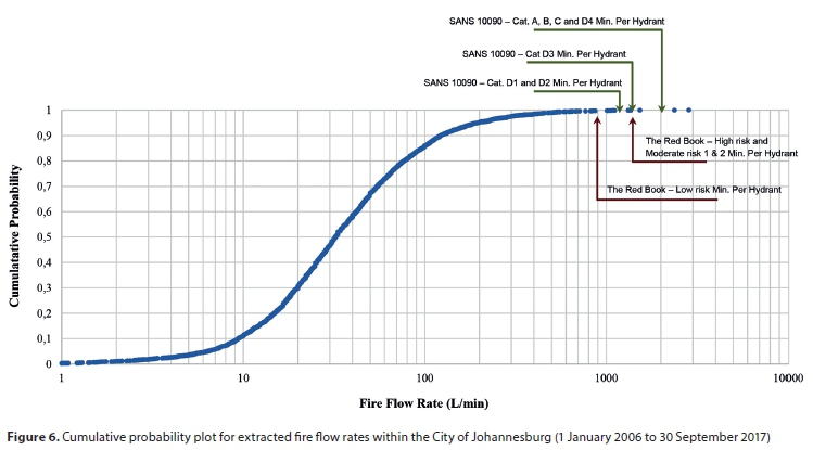
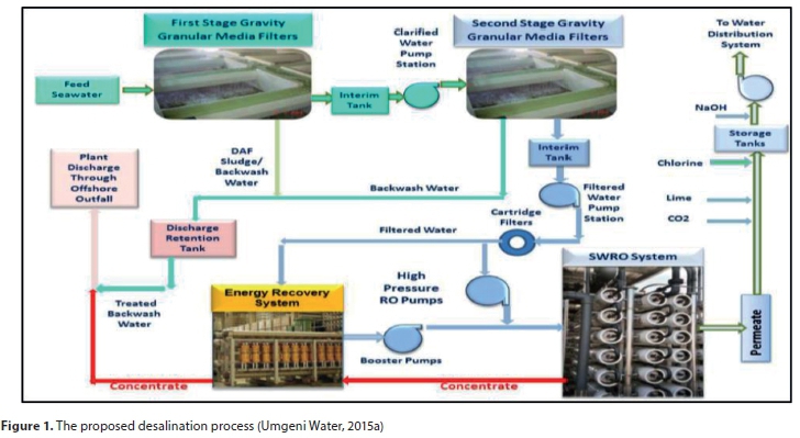
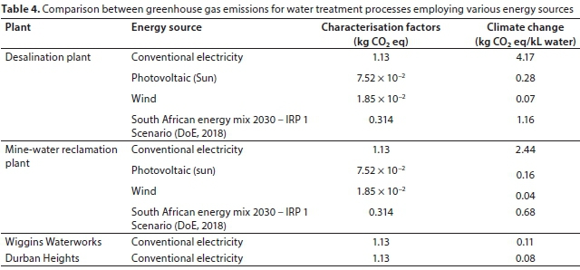
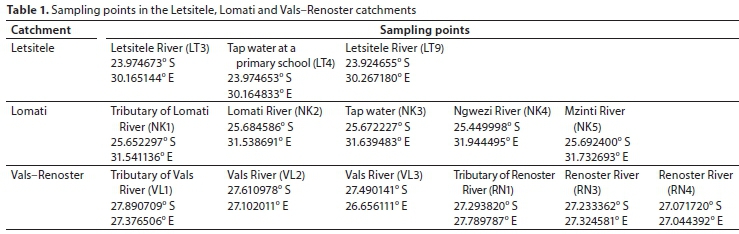
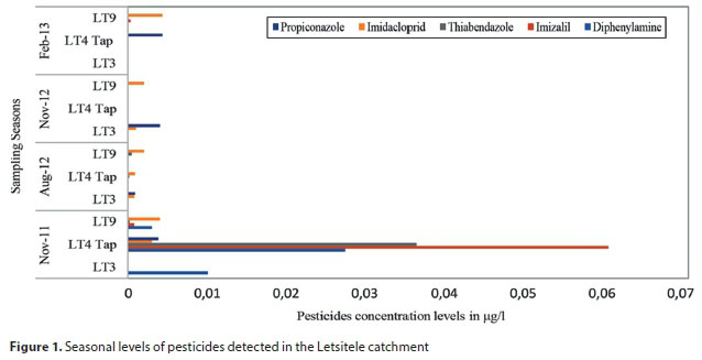
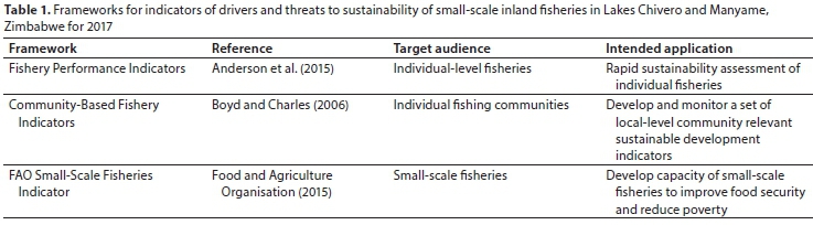