RESEARCH PAPERS

 

Garden irrigation as household end-use in the presence of supplementary groundwater supply

 

 

Bettina Elizabeth Meyer; Heinz Erasmus Jacobs^*

Department of Civil Engineering, Stellenbosch University, Private Bag X1, Matieland, 7602, South Africa

 

 

---

ABSTRACT

Garden irrigation is a significant and variable household water end-use, while groundwater abstraction may be a notable supplementary water source available in some serviced residential areas. Residential groundwater is abstracted by means of garden boreholes or well points and - in the study area - abstracted groundwater is typically used for garden irrigation. The volume irrigated per event is a function of event duration, frequency of application and flow rate, which in turn are dependent on numerous factors that vary by source - including water availability, pressure and price. The temperature variation of groundwater abstraction pipes at residential properties was recorded and analysed as part of this study in order to estimate values for three model inputs, namely, pumping event duration, irrigation frequency, and flow rate. This research incorporates a basic end-use model for garden irrigation, with inputs derived from the case study in Cape Town, South Africa. The model was subsequently used to stochastically evaluate garden irrigation. Over an 11-d period, 68 garden irrigation events were identified in the sample group of 10 residential properties. The average garden irrigation event duration was 2 h 16 min and the average daily garden irrigation event volume was 1.39 m³.

Keywords: garden irrigation, end-use, groundwater, residential water demand

---

 

 

INTRODUCTION

Residential water consumption is typically categorised into indoor end-uses and outdoor end-uses. Previous studies suggest outdoor use to be seasonal, driven by weather-related variables, whilst indoor use has been found to be relatively constant (FisherJeffes et al., 2015). Outdoor use is also considered more unpredictable than indoor use (Hemati et al., 2016). Howe and Linaweaver (1967), in an early study of residential water demand, reported on the inelastic nature of indoor water use versus the elastic nature of outdoor use, meaning that outdoor use was found to be more sensitive to a change in inputs than indoor use. Jacobs and Haarhoff (2007) used elasticity and a sensitivity parameter to identify pan evaporation, an irrigation factor, lawn surface area (lawn size) and the vegetation crop factor (lawn grass genotype) as the most notable parameters when modelling outdoor water use.

Various parameters describing outdoor use have received attention as part of earlier work, including garden irrigation (Beal et al., 2011), lawn size (Runfola et al., 2013), swimming pools (Fisher-Jeffes et al., 2015), and water use from the outside tap (Makwiza and Jacobs, 2017). Household water leakage was also addressed in earlier work (Britton et al., 2008; Lugoma et al., 2012). The most notable outdoor end-use in an unrestricted scenario is garden irrigation. Garden irrigation is often reported as a notable part of the total per-capita consumption (Willis et al., 2011). It is unsurprising that outdoor use is the primary target during water restrictions, with earlier studies reporting on reduced water use during water restrictions, mainly due to reduced outdoor use (Jacobs et al., 2007).

Despite the attention to various facets of outdoor use in earlier work, end-use studies have paid limited attention to water supply from supplementary household water sources (Nel et al., 2017). This research focuses on modelling garden irrigation as an end-use in an unrestricted scenario, where groundwater was abstracted from privately owned groundwater abstraction points (GAPs) as supplementary water source. Residential GAPs include garden boreholes and relatively shallow wellpoints.

Consumers may turn to alternative non-potable water sources such as rainwater, groundwater or greywater during stringent water restrictions. The quality of these resources typically limits application to nonpotable uses, such as garden irrigation (MacDonald and Calow, 2009). According to Nel et al. (2017), groundwater use is the most notable supplementary source in terms of the expected supply volume. Many privately owned GAPs are in use across South Africa, with at least one notable case study in the Cape Town region (Wright and Jacobs, 2016). Monitoring of household groundwater abstraction in South Africa is poor and published information regarding yield, flow rate, and/or the pumping event duration of household GAPs is limited.

Garden irrigation as outdoor end-use

The contribution of garden irrigation to the total household water use varies by season (Parker and Wilby, 2013) and also varies from country to country and even from house to house. Garden irrigation tends to be higher during dry, hot seasons, and increases with reduced rainfall (Jacobs and Haarhoff, 2004; Parker and Wilby, 2013) and increased maximum daily temperatures (Rathnayaka, 2015), for example. The garden event duration and number of occurrences are contingent on the method of irrigation. Roberts (2005) identified three main irrigation methods, namely, hand-held hose, manual sprinkler and automated sprinkler. The latter contributed most to garden irrigation volumes from the end-use study conducted by Roberts (2005) in Australia. The same three irrigation methods were found in the study area during this research.

Literature includes various reports of garden irrigation expressed as a percentage of the total household water demand, in order to explain the significant contribution of garden irrigation to total household water use. The perceived percentage of residential water demand used for garden irrigation in South Africa, based on an annual average, was reported to vary between 0% and 70% (Veck and Bill, 2000). More recent end-use studies conducted in South Africa reported the percentage of average annual household water demand ascribed to garden irrigation as 40% to 60% (Du Plessis and Jacobs, 2015) and 58% (Du Plessis et al., 2018) in different South African study samples.

End-use studies conducted in other parts of the world also report a wide range of values expressing garden irrigation as a percentage of the total household water use. In Australia, the percentage of household water demand used for garden irrigation ranges from 5% (Beal et al., 2011) to 54% (Loh and Coghlan, 2003). Arbon et al. (2014) reported a strong seasonal impact in Adelaide, Australia, with a 2013 winter mean of 153 L/person per day increasing to 498 L/person per day in the summer of 2013/14. The average annual use was 245 L/person per day and 289 L/person per day in 2013 and 2014 respectively, that could indicate a garden irrigation contribution of 50% to 70% of the total annual household demand; a significant shift in the diurnal pattern was noted, with an afternoon peak more prominent during summer. A lower outdoor use contribution of 15% was reported at high-income detached houses by Ghavidelfar et al. (2018) in Auckland, New Zealand. Wasowski (2001) conducted an end-use study in the United States of America and stated that between 40% and 60% of annual average residential water demand is attributed to garden irrigation.

Rationale

Suburban households in the case study area of Cape Town, South Africa, are accustomed to a reliable supply of potable water from the pressurised water distribution system. However, the rising block-based water tariff was relatively high and, also, outdoor water use from the distribution system was banned during water restrictions in the study area - for the period June 2017 to December 2018. Consumers subjected to emergency water restrictions turned to alternative sources of water to maintain gardens during this 18-month period. Little is known about garden water use by consumers with access to groundwater from garden GAPs; the restrictions provided the opportune time to investigate the matter. The main challenge in this study was to obtain data regarding actual groundwater use by private homeowners, who were often reluctant to share any information regarding uncontrolled and unmetered household water sources.

Research problem

An end-use model was needed to assess garden irrigation in relation to supplementary groundwater supply, while populating the model with data that could realistically represent the key unknowns.

 

METHODS

Parameters describing the quantity and quality of household groundwater abstraction form important inputs to end-use models of household water use. Groundwater use for garden irrigation was modelled in this study, with inputs based on measured values. Data were collected from a relatively small case study site in Cape Town, South Africa. Direct measurement of groundwater abstraction was not considered feasible and an alternative method to assess the volume of groundwater abstracted for garden irrigation was employed.

Groundwater pumping event start times and durations were derived from continuously recorded pipe wall temperatures at each of the 10 residential properties. Ad hoc volumetric measurements were subsequently conducted at each home to gain insight into flow rates at each study home. Stochastic end-use modelling was employed to estimate the expected garden irrigation event volume of the 10 properties in the research sample. Based on information obtained during the site survey, garden irrigation volume was considered to be equal to the groundwater abstracted from GAPs for all homes in the case study.

Overview of residential end-use models

The focus of this study was on modelling water demand at a small spatial scale of single residential homes - and garden irrigation as a specific end-use of water. Numerous residential end-use models have been developed in the past; however, a model to evaluate garden irrigation in relation to groundwater abstraction as supplementary source has not yet been developed. Some examples of earlier end-use models include the Poisson Rectangular Pulse (PRP) model developed by Buchberger et al. (1996; 2003), the SIMulation of Demand End-Use Model (SIMDEUM) by Blokker et al. (2010) and the Residential End-Use Model (REUM) by Jacobs and Haarhoff (2004). REUM and SIMDEUM incorporate garden irrigation as end-use.

Experimental field tests and data analysis

Study site selection and sample group

A map of verified residential properties with GAPs in the Cape Town Metropolitan area was developed by Wright and Jacobs (2016). The sample group of 10 homes for this study was based on sub-regions where clustering of GAPs (as reported by Wright and Jacobs, 2016) was observed, followed by personal invitation to participate in the study. Relatively small sample sizes are not unusual for end-use studies. Former end-use studies had sample sizes of 28 homes (Butler, 1991), 16 homes (DeOreo et al., 1996), 37 homes (DeOreo et al., 2001), 21 homes (Buchberger et al., 2003), 12 homes (Heinrich, 2007), 10 homes (Jacobs, 2007) and 10 homes (Mead and Aravinthan, 2009).

The manageable sample size in this study also enabled the authors to inspect individual pump installations for leaks and to conduct follow-up inspections. All the houses in the sample were single residential properties, with property plot sizes ranging from 600 m² to 1 400 m². Prominent, well-irrigated gardens and lawns were present at all homes. Two residential properties from the study site each had a swimming pool; however, the homeowners assured that the abstracted groundwater was explicitly used for garden irrigation at the time of this study. The assumption that groundwater supply equalled garden irrigation was thus considered valid for the study sample. The addresses and suburb names of the study homes were omitted for anonymity, in line with ethical requirements.

Data collection methods

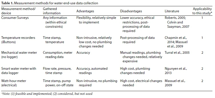
Residential water demand patterns should preferably be obtained by measuring actual water use (Scheepers and Jacobs, 2014); however, empirical investigations involving data collection are often faced with several logistical, time and financial constraints. Various data collection methods were considered for this study in order to collect sensitive information that was needed to assess household groundwater abstraction. A list of empirical measurement methods is presented in Table 1, including the key advantages and disadvantages in each case, as well as a reference to earlier application. Each method was categorised in terms of feasibility as it relates to the case study. Two categories were included, namely: (1) considered for this case study and also implemented in the study; (2) considered for this study, but not used.

Equipment and temperature recording

The project plan involved recording pipe wall temperature at case study homes in an unobtrusive way, with no plumbing requirements, a short installation time and relatively low cost. The DS1922 Thermochron Hi Resolution iButton was selected for this study, based on the relatively small size, ruggedness, accuracy, cost, and availability. The iButtons were used in this study to measure the variation in temperature of the groundwater pump delivery pipe - that is the delivery pipe of the GAP pump supplying water directly for garden irrigation. The temperature variations were subsequently used to assess water use events by determining the event duration of groundwater pumping, start and stop times.

The iButtons were preconfigured to set the start time and sample rate. ColdChain ThermoDynamics software was used for preconfiguration and to extract and save the recorded data. All the iButtons were programmed to have a sampling rate of 2 min, which was considered sufficient when compared to the relatively long events. The period of 2 min was the shortest interval available when programming the equipment. The iButtons were synchronised to start at the same time on the same date. The internal iButton memory allowed for a total recording duration of 11 d and 9 h (sample count of 8 192 records per iButton). After the iButtons were activated and before the specified start time, the iButtons were installed on the outside wall of the outlet pipe, using adhesive electrical tape. Each GAP was equipped with two synchronous iButtons to record temperature in parallel. The sample included 10 homes and data were recorded during April and May 2016. Subsequently the total data set included 110 test days, representing 11 actual calendar days for each of the 10 homes.

The iButtons were placed in three different environments (A, B, and C). Each environment type was linked to an installation that affected the temperature changes of the iButtons differently. In Environment A the pump and outlet pipes were located in an enclosure that was not exposed to any sunlight. A typical Environment A would be described as a well-insulated concrete pump house with an access door. Due to the insolation, the ambient temperature fluctuation within the enclosure was moderate. Environment B would have the pump and outlet pipes protected from direct sunlight and precipitation by means of a four-walled, wooden or steel enclosure. Access to the equipment was provided via a removable roof. The shape and size of the enclosure is similar to that of a typical medium-sized doghouse. Environment B was found to be relatively similar to Environment A in terms of temperature fluctuation within the enclosure. In Environment C, the pump and outlet pipes were exposed to direct sunlight and therefore experienced more notable ambient temperature changes compared to the other two environments. The sample group had two GAPs located in an Environment A, six GAPs in an Environment B and two GAPs in an Environment C.

Flow intensity measurements

The intensity (flow rate) was determined at each GAP, using on-site volumetric measurements. The measurement entailed filling a container with water at the endpoint of the irrigation pipe. The container was filled for 45 s and subsequently weighed. The container was weighed pre- and post-fill and the flow rate was calculated. The manageable sample size allowed for a sufficient number of volumetric measurements. Each measurement was repeated 10 times at each GAP, resulting in 100 flow rate measurements. The measurements were used to create a distribution graph, representing the flow intensities for the study site. This method was easily executed, cost effective and caused little disturbance to the residents.

Consumer surveys

Surveys have been used in the past as an indication of indoor (Blokker et al., 2010) and outdoor water use (Roberts, 2005; Veck and Bill, 2000). A site survey was conducted as part of this study to obtain relevant information regarding water-use activities, including identification of the irrigation method (hand-held hose, manual sprinkler, automatic sprinkler), system connectivity, pump placement environment and water leakage. Although the method of irrigation was documented in the survey, it was not incorporated into the end-use model due to the limited sample size. The site surveys were also used to confirm that the residents used the irrigation systems at the maximum flow rate in each case. The pump flow rate was assumed equal to the garden irrigation flow rate in each case, with no leakage reported at any site.

Identifying pumping events and durations

Adopting terminology from Jacobs and Haarhoff (2004), the number of events over a given time period was described by using the term 'event frequency', expressed as the number of events per day. The term 'event duration' was used to describe the time lapse from an event start to event end. The recorded pipe wall temperature was analysed in order to identify pumping events and to extract the event frequency and event duration. The procedure was termed temperature variation analysis. Since temperature on each pipe was separately measured and analysed, there were no overlapping events. Each pumping event represented a single garden irrigation occurrence and was characterised by the pump start operation (water flowing through the pipe with corresponding temperature change) and the pump being turned off again. A Visual Basic macro, for implementation in MS Excel, was written to implement the temperature variation calculations. The baseline temperature, needed to identify significant interruptions in the expected graph pattern, was first established. Each interruption (difference between pipe wall temperature and baseline temperature) corresponded to a pumping event.

The daily ambient temperature fluctuated over the study period. The fluctuations varied per installation, because each iButton was placed in a different environment. Consequently, the baseline temperature at each GAP varied. The developed baseline temperature time-series graph at each GAP represented the typical daily temperature cycle per installation. The coefficient of determination (R²) was used as a measure of similarity in shape between the baseline temperature at each GAP, and the temperature measured on the pipe wall. Thus each GAP had a specific baseline temperature corresponding to the particular environment and the ambient temperature of the specific day. After the baseline temperature was developed, pumping events and durations were identified. Figure 1 shows an example of the pipe wall temperature measured by an iButton, and the corresponding baseline temperature curve, for one property over a 2-d period. The selected time series shows two events. A pumping event is noticed at about 06:00 on both days.

During time steps where the measured pipe wall temperature and baseline temperature deviated notably, water was likely flowing through the pipe (evidence of an event). Firstly, the temperature noise in each environment had to be separated from notable temperature deviations. Figure 2(a) shows the difference between the derived baseline temperature and the pipe wall temperature. Temperature noise is clearly visible around the zero y-axis value. In order to automatically detect pumping events, a conditional filter, incorporating a threshold temperature, was applied. The threshold value was determined with consideration for the different environments in which the iButtons were placed, being informed by earlier studies. Massuel et al. (2009) used a threshold of 2.6°C to detect pumping events as part of a study in India. In this study, the threshold was set equal to 2.0°C for Environment A and Environment B and to 3.0°C for Environment C. Implementing the threshold allowed for pumping events to be identified with an algorithm, which is significantly less time consuming than manual interpretation of the recorded data. With reference to the temperature noise visible in Fig. 2(a), all values not exceeding the threshold temperature were set equal to 0 and the result is plotted in Fig. 2(b). Figure 2(b) shows the two individual events in the selected time series, excluding temperature noise below the selected threshold values.

 

 

All recorded data were analysed in this manner by employing the algorithm. In total, 68 individual events were identified on 59 test days, considering the full data set of 110 test days. Multiple irrigation events per day were detected at only one home. The highest event frequency was 3 events per day, reported only once; 2 events per day were reported 7 times in the full data set at the same home. The limited number of events reported on in this study also allowed for subsequent visual inspection of the temperature difference at each event.

Basic model structure

A rudimentary model was developed to stochastically determine the average daily volume of groundwater pumped for garden irrigation. The model included three independent parameters (duration, frequency, intensity) and was termed the DFI model. The DFI model adopted notation from the SIMDEUM model developed by Blokker et al. (2010), and is based on the assumption that all the input parameters are independent and statistically distributed random variables.

The DFI model structure, for a single residential property, is described by Eq. 1:

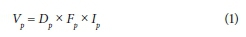
where,

V = average daily garden irrigation event volume (m³/d)

D = event duration (h/event)

F = event frequency (events/d)

I = flow intensity (flow rate) at GAP (m³/h)

The subscript p represents the best-fit probability distribution type of the respective variables in the DFI model. The procedure of setting up a stochastic model with the known distributions for each variable involved an evaluation of each model input parameter in terms of suitable statistical distributions.

Stochastic description of parameters

The best-fit statistical distributions for D, F, and I, were selected by implementing goodness-of-fit (GOF) tests to the measured data, using @Risk software. The GOF tests included the Anderson-Darling, Kolmogorov-Smirnov and Chi-Squared statistic. The best-fit distribution was chosen based on a combined scoring system of the GOF tests, similar to the selection tool developed by Masereka et al. (2015). The fitted statistical distributions used in the DFI model are presented in Table 2, along with the corresponding mathematical descriptions and parameters.

 

 

RESULTS

Experimental field test results

Results discussed in this section were obtained from temperature variation analysis and volumetric measurements. A total of 68 irrigation events were identified over the 11-d study period by means of the temperature variation analysis. The average garden irrigation event duration was 2 h 16 min, with a relatively large standard deviation of 1 h 17 min. The longest irrigation event measured was 6 h and 59 min, and the shortest was 22 min. Some events were found to be relatively long in comparison with garden irrigation events reported elsewhere. The consumers of this study sample confirmed that, in some cases, the GAP would be operated until the aquifer was (temporarily) depleted and the event had to be terminated to allow for recharge, resulting in relatively long events.

The probability of an irrigation event occurring on a specific day during the 110 test days in the sample was 54%, meaning that consumers irrigated roughly every second day, on average. The flow intensities at the GAPs ranged between 1.14 m³/h and 1.25 m³/h, with a most likely value of 1.16 m³/h. These values were considered to be typical for groundwater abstraction at the household scale in South Africa. Local borehole contractors often use a thumb rule of 1 L/s (3.6 m³/h) as a relatively good flow rate from a garden borehole pump. Tennick (2000) reported that garden borehole flow rates in Hermanus, South Africa, ranged between 1 m³/h and 2 m³/h. Naidoo and Burger (2017) also reported on groundwater abstraction in South Africa. The average pump flow rate was found to range between 0.36 m³/h and 2.7 m³/h (Naidoo and Burger, 2017). Flow intensity values from this study were thus within the range reported earlier.

Stochastic results

Event duration

Garden irrigation event duration D was determined by means of the temperature variation analysis procedure described earlier. Many factors may contribute to the duration of irrigation, including the method of irrigation, property size, rainfall, aquifer yield, ambient temperature and time of day. These factors were not considered in the DFI end-use model; event duration was modelled as an independent variable. If multiple events occurred on the same day, each event duration was analysed separately.

A cumulative distribution function (CDF) of the measured duration is presented in Fig. 3, along with the CDF of the stochastic distribution with the best fit. The loglogistic distribution provided the best fit, slightly outperforming the lognormal distribution that ranked second in terms of fit. However, the parameters of the lognormal distribution (mean and standard deviation) are more readily available than the shape and scale parameters of the log-logistic distribution. Therefore, the lognormal distribution was selected to model the irrigation duration variable, thus simplifying practical application in the future.

 

 

Event frequency

Event frequency F is often described using a discrete statistical distribution (Blokker et al., 2010) and is typically expressed as a Poisson distribution, in which case only one parameter is needed (λ = average) to populate the distribution. The event frequency was modelled as the probability of a garden irrigation event occurring on a specific day, with a maximum of 1 pumping event per day. Consequently, the binomial distribution was used to describe event frequency over the 11-d study period. Figure 4 shows the CDF of the measured irrigation frequencies with the fitted binomial distribution curve.

 

 

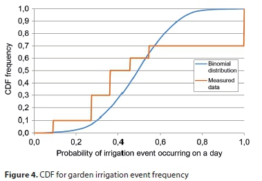
No distribution fitted the measured data well, partly because of the small sample size and relatively sustained consumer habits and/or the use of automated programmed irrigation timers. Many different events from a particular home would thus report the same frequency and would be lumped in the CDF. The significant difference between event irrigation frequencies could also be ascribed in part to consumer behaviour and also to the different types of irrigation systems used at the study homes. The irrigation method was, however, not included as independent variable in the DFI model. Additionally, no rain days occurred during the study period. The binomial distribution provided the best fit to the data and was considered adequate to illustrate application of the model, with appreciation that future research in this regard is needed.

Flow intensity

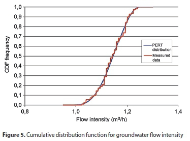
The site survey confirmed that all GAPs were operated at full capacity while irrigating. Thus the flow intensity I at each GAP was measured at the maximum flow rate. A CDF, containing 100 data points (10 measurements at each of the 10 residential properties) was plotted in Fig. 5. The Beta-Program Evaluation and Review Technique (PERT) distribution, identified as the best fit to the actual data, was superimposed on the actual data. The PERT distribution incorporates three parameters: the minimum, maximum, and the most likely value.

 

 

Application of DFI model to study site

Statistical distributions were fitted to measurements obtained from the iButtons and volumetric measurements. Equation 1 was modified to include the identified best-fit distributions for each model variable. Equation 2 represents the stochastic DFI model:

Table 3 summarises the variables of the DFI model, as well as the parameter values of the specific study site. The parameter values in Table 3 represent garden irrigation in autumn for the specific Cape Town study site.

 

 

The DFI model was implemented on the study site by populating Eq. 2 with the values presented in Table 3. A total of 1 000 000 iterations were simulated using the Monte Carlo method to stochastically determine the average daily volume (in m³/d) of groundwater pumped for garden irrigation. The CDF of the average daily garden irrigation event volume supplied from GAPs at the study site is shown in Fig. 6. A comparison of the DFI model's stochastic results (based on GOF tests) and the study site measurements is presented in Fig. 6.

 

 

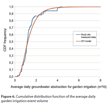
The results presented in Fig. 6 relate to the study site over the study period (April/May) and should not be generalised. The average daily groundwater abstraction for garden irrigation could simply be calculated by multiplying the average values of D, F, and I. The stochastic results also show that a daily average of 1.39 m³/d is used for garden irrigation, as would be expected. Due to the relatively large variation in garden irrigation volume, from one home to the next, one region to the other and by season, the average value alone does not provide sufficient insight. The stochastic results provide more detail. An additional sensitivity analysis was conducted in order to explain the relative contribution of different parameter values. The sensitivity analysis showed that garden irrigation volume was the most sensitive to event duration. The significant contribution of event duration in the model is explained by the notable parameter variability coupled to a relatively wide range in event duration amongst residents.

 

DISCUSSION

Utilising iButtons as indirect method for measuring water usage at privately owned GAPs proved useful. The method was simple, cost effective and caused relatively little disturbance to the homeowners. The average pumping event duration at the study site was 2 h and 16 min, with the shortest event being 22 min. The recording interval of 2 min ensured that irrigation events could successfully be identified, because event duration significantly exceeded the recording interval. Expanding the application of iButtons to include different household end-use components, such as the bath, shower, washing machine and dishwasher could be explored. However, iButtons would be unable to detect events with a relative short duration (less than 2 min), such as basin taps and toilet flushing, or events where the temperature variation is expected to be small. The temperature variation method has been applied to hot water end-uses, such as the shower (Botha et al., 2017), where temperature variation is expected to be relatively large.

The average irrigation duration and frequency measured in this study are higher than values reported by Roberts (2005). This research project focused on groundwater as supplementary water source, meaning that an unrestricted irrigation scenario was considered. Consequently, it could be expected that residents with GAPs (this study) would irrigate more regularly and for longer durations compared to a sample group of residents using water from the potable water distribution system for garden irrigation.

The DFI model can serve as a useful, rudimentary means to investigate garden irrigation by researchers and utility managers. Based on the relatively small sample of 59 measurement points, a probability distribution function (PDF) cannot be defined with sufficient representativeness for longer time periods, or other regions. The combination of literature values and the 59 data points was used in this study to compile PDFs as a means to illustrate the method and obtain results from the study sample. The results are not representative of a larger region, or consumers beyond the study site. However, the DFI model is scalable over different study sites, as the parameters of the distribution curves could be populated with values corresponding to another region, or time, as applicable. The DFI model could be expanded in the future to incorporate seasonal variability, different irrigation methods and also other types of supplementary household water supply, such as rainwater and greywater.

 

CONCLUSION

Unique garden irrigation events from groundwater abstraction points were identified by means of temperature variation analysis in the Cape Town case study site. A relatively high garden irrigation event occurrence was observed at all 10 homes and the recorded duration of the 68 detected events was relatively long. The DFI model was based on data measured in the Cape Town study site and was subsequently used to illustrate stochastic modelling of garden irrigation. The temperature variation analysis could be employed elsewhere to populate the DFI model with values for event duration, frequency and intensity (flow rate) in order to assess garden irrigation from groundwater abstraction points in other regions.

 

ACKNOWLEDGEMENTS

The authors would like to thank the National Research Foundation (NRF) of South Africa and GLS Consulting for financial support towards a post-graduate student bursary.

 

REFERENCES

ARBON N, THYER M, HATTON MACDONALD D, BEVERLEY K and LAMBERT M (2014) Understanding and predicting household water use for Adelaide. Technical Report Series No. 14/15. Goyder Institute for Water Research, Adelaide, South Australia.         [ Links ]

BEAL C, STEWART RA, HUANG T and REY E (2011) South East Queensland residential end use study. J. Aust. Water Assoc. 38 (1) 80-84.         [ Links ]

BLOKKER EJM, VREEBURG JHG and VAN DIJK JC (2010) Simulating residential water demand with a stochastic end-use model. J. Water Resour. Plann. Manage. 136 19-26. https://doi.org/10.1061/(asce)wr.1943-5452.0000002        [ Links ]

BOTHA BE, JACOBS HE, BIGGS B and ILEMOBADE AA (2017) Analysis of shower water use and temperature at a South African university campus. CCWI 2017 - Computing and Control for the Water Industry, 5-7 September 2017, Sheffield, United Kingdom. https://doi.org/10.15131/shef.data.5364562.v1        [ Links ]

BRITTON T, COLE G, STEWART R and WISKAR D (2008) Remote diagnosis of leakage in residential households. J. Aust. Water Assoc. 35 89-93.         [ Links ]

BUCHBERGER SG and WELLS GJ (1996) Intensity, duration, and frequency of residential water demands. J. Water Resour. Plann. Manage. 112 (1) 11-19. https://doi.org/10.1061/(asce)0733-9496(1996)122:1(11)        [ Links ]

BUCHBERGER SG, CARTER JT, LEE YH, and SCHADE TG (2003) Random demands, travel times, and water quality in dead ends. Rep. No. 90963F. AWWARF, Denver.         [ Links ]

BUTLER JJ (1991) A stochastic analysis of pumping tests in laterally nonuniform media. Water Resour. Res. 27 (9) 2401-2414. https://doi.org/10.1029/91wr01371        [ Links ]

CHAPMIN T, TODD AS and ZEIGLER MP (2014) Robust, low-cost data loggers for stream temperature, flow intermittency, and relative conductivity monitoring. Water Resour. Res. 50 (8) 6542-6548. https://doi.org/10.1002/2013wr015158        [ Links ]

COLVIN C and SAAYMAN I (2007) Challenges to groundwater governance: a case study of groundwater governance in Cape Town, South Africa. Water Polic. 9 (2) 127-149. https://doi.org/10.2166/wp.2007.129        [ Links ]

DEOREO WB, HEANEY JP and MAYER PW (1996) Flow trace analysis to assess water use. J. Am. Waste Water Assoc. 88 (1) 79-90.         [ Links ]

DEOREO WB, DIETERMANN A, SKEEL T, MAYER PW, LEWIS DM and SMITH J (2001) Retrofit realties. J. Am. Water Works Assoc. 93 (3) 58-72.         [ Links ]

DU PLESSIS JL and JACOBS HE (2015) Procedure to derive parameters of stochastic modelling of outdoor water use in residential estates. Proced. Eng. 119 803-812. https://doi.org/10.1016/j.proeng.2015.08.942        [ Links ]

DU PLESSIS JL, FAASEN B, JACOBS HE, KNOX AJ and LOUBSER C (2018) Investigating wastewater flow from a gated community to disaggregate indoor and outdoor water use. J. Water Sanit. Hyg. Dev. 8 (2) 238-245. https://doi.org/10.2166/washdev.2018.125        [ Links ]

FISHER-JEFFES L, GERTSE G and ARMITAGE NP (2015) Mitigating the impact of swimming pools on domestic water demand. Water SA 41 (2) 238-246. https://doi.org/10.4314/wsa.v41i2.9        [ Links ]

GHAVIDELFAR S, SHAMSELDIN AY and MELVILLE BW (2018) Evaluating spatial and seasonal determinants of residential water demand across different housing types through data integration. Water Int. 43 (7) 926-942. https://doi.org/10.1080/02508060.2018.1490878        [ Links ]

HEMATI A, RIPPY M, GRANT S, DAVIS K and FELDMAN D (2016) Deconstructing demand: the anthropogenic and climatic drivers of urban water consumption. Environ. Sci. Technol. 50 (23) 12557-12566. https://doi.org/10.1021/acs.est.6b02938        [ Links ]

HEINRICH M (2007) Water end use and efficiency project (WEEP) - Final report. BRANZ Study report 159. BRANZ, Judgeford, New Zealand.         [ Links ]

HOWE CW and LINAWEAVER FP (1967) The impact of price on residential water demand and its relation to system design and price structure. Water Resour. Res. 3 (1) 13-32. https://doi.org/10.1029/wr003i001p00013        [ Links ]

JACOBS HE (2007) The first reported correlation between end-use estimates of residential water demand and measured use in South Africa. Water SA 33 (4) 549-558.         [ Links ]

JACOBS HE and HAARHOFF J (2007) Prioritisation of parameters influencing residential water use and wastewater flow. J. Water Supply: Res. Technol. 56 (8) 495-514. https://doi.org/10.2166/aqua.2007.068        [ Links ]

JACOBS HE AND HAARHOFF J (2004) Structure and data requirements of an end-use model or residential water demand and return flow. Water SA 30 (3) 293-304. https://doi.org/10.4314/wsa.v30i3.5077        [ Links ]

JACOBS HE, GEUSTYN LC, FAIR K, DANIELS J and DU PLESSIS JA (2007) Analysis of water savings: a case study during the 2004/2005 water restrictions in Cape Town. J. S. Afr. Inst. Civ. Eng. 49 (3) 16-26.         [ Links ]

LOH M and COGHLAN P (2003) Domestic water use study in Perth, Western Australia (1998-2001). March 2003. Water Corporation, Perth, Australia. ISBN 1 74043 1235        [ Links ]

LUGOMA MFT, VAN ZYL JE and ILEMOBADE AA (2012) The extent of on-site leakage in selected suburbs of Johannesburg. Water SA 38 (1) 127-132. https://doi.org/10.4314/wsa.v38i1.15        [ Links ]

MACDONALD AM and CALOW RC (2009) Developing groundwater for secure water supplies in Africa. Desalination 248 546-556. https://doi.org/10.1016/j.desal.2008.05.100        [ Links ]

MAKWIZA C and JACOBS HE (2017) Sound recording to characterize outdoor tap water use events. J. Water Suppl.: Res. Technol. 66 (6) 392-402. https://doi.org/10.2166/aqua.2017.120        [ Links ]

MASEREKA EM, OTIENO FAO, OCHIENG GM and SNYMAN J (2015) Best fit selection of probability distribution models for frequency analysis of extreme mean annual rainfall events. Int. J. Eng. Res. Dev. 11 (4) 34-53.         [ Links ]

MASSUEL S, PERRIN J, WAJID M, MASCRE C and DEWANDEL B (2009) A simple low-cost method to monitor duration of groundwater pumping. Groundwater 41 (1) 141-145. https://doi.org/10.1111/j.1745-6584.2008.00511.x        [ Links ]

MEAD N and ARAVINTHAN V (2009) Investigation of household water consumption using smart metering system. Desalination Water Treat. J. 11 (1-3) 115-123. https://doi.org/10.5004/dwt.2009.850        [ Links ]

NAIDOO V and BURGER M (2017) Groundwater abstraction assessment for development on the farm Vlakfontein 523 JR Portion 25. Report compiled for JCJ Developments. Geo Pollution Technologies Report No. ICEAS-17-2246. JCJ Developments, Gauteng, South Africa.         [ Links ]

NEL N, JACOBS HE, LOUBSER C and DU PLESSIS JA (2017) Supplementary household water sources to augment potable municipal supply. Water SA 43 (4) 553-562. https://doi.org/10.4314/wsa.v43i4.03        [ Links ]

PARKER JM and WILBY RL (2013) Quantifying household water demand: A review of theory and practice in the UK. Water Resour. Manage. 27 (4) 981-1011. https://doi.org/10.1007/s11269-012-0190-2        [ Links ]

RATHNAYAKA K (2015) Seasonal demand dynamics of residential water end-uses. Water J. 7 202-216. https://doi.org/10.3390/w7010202        [ Links ]

ROBERTS P (2005) Yarra Valley Water 2004 residential end use measurement study. Final report, June 2005. Yarra Valley Water. Melbourne, Australia.         [ Links ]

RUNFOLA DM, POLSKY C, NICOLSON C, GINER NM, PONTIUS RG, KRAHE J and DECATUR A (2013) A growing concern? Examining the influence of lawn size on residential water use in suburban Boston, MA, USA. Landscape Urban Plann. J. 119 113-123. https://doi.org/10.1016/j.landurbplan.2013.07.006        [ Links ]

SCHEEPERS HM and JACOBS HE (2014) Simulating residential indoor water demand by means of a probability based end-use model. J. Water Supply: Res. Technol. 63 (6) 476-488. https://doi.org/10.2166/aqua.2014.100        [ Links ]

TENNICK FP (2000) Preliminary report on hydrocensus of groundwater resources in the Eastcliff and Northcliff suburbs, Hermanus, Western Cape, South Africa. Compiled by FPT Consulting Services for the Overstrand Municipality, May 2000.         [ Links ]

TURRAL HN, ETCHELLS T, MALANO HMM, WIJEDASA HA, TAYLOR P, MACMAHON TAM and AUSTIN N (2005) Water trading at the margin: The evolution of water markets in the Murray-Darling Basin. Water Resour. Res. 41 W07011. https://doi.org/10.1029/2004wr003463        [ Links ]

VECK GA and BILL MR (2000) Estimation of the residential price elasticity of demand for water by means of a contingent evaluation approach. WRC Report No. 790/1/00. Water Research Commission, Pretoria.         [ Links ]

WASOWSKI A (2001) Changing the American landscape. J. Am. Wastewater Assoc. 3 40-44.         [ Links ]

WILLIS RM, STEWART RA, PANUWATWANICH K, WILLIAMS PR and HOLLINGSWORTH AL (2011) Quantifying the influence of environmental and water conservation attitudes on household end use water consumption. J. Environ. Manage. 92 (8) 1996-2009. https://doi.org/10.1016/j.jenvman.2011.03.023        [ Links ]

WRIGHT T and JACOBS HE (2016) Potable water use of residential consumers in the Cape Town metropolitan area with access to groundwater as supplementary household water source. Water SA 42 (1) 144-150. https://doi.org/10.4314/wsa.v42i1.14        [ Links ]

 

 

Received 5 Feb 2018
Accepted in revised form 27 May 2019

 

 

* Corresponding author, email: hejacobs@sun.ac.za