RESEARCH PAPERS

 

Assessment of CFD turbulence models for free surface flow simulation and 1-D modelling for water level calculations over a broad-crested weir floodway

 

 

Ahmed M Helmi^*

Irrigation and Hydraulics Department, Faculty of Engineering, Cairo University, Egypt

 

 

---

ABSTRACT

Floodways, where a road embankment is permitted to be overtopped by flood water, are usually designed as broad-crested weirs. Determination of the water level above the floodway is crucial and related to road safety. Hydraulic performance of floodways can be assessed numerically using 1-D modelling or 3-D simulation using computational fluid dynamics (CFD) packages. Turbulence modelling is one of the key elements in CFD simulations. A wide variety of turbulence models are utilized in CFD packages; in order to identify the most relevant turbulence model for the case in question, 96 3-D CFD simulations were conducted using Flow-3D package, for 24 broad-crested weir configurations selected based on experimental data from a previous study. Four turbulence models (one-equation, k-ε, RNG k-ε, and k-ω) ere examined for each configuration. The volume of fluid (VOF) algorithm was adopted for free water surface determination. In addition, 24 1-D simulations using HEC-RAS-1-D were conducted for comparison with CFD results and experimental data. Validation of the simulated water free surface profiles versus the experimental measurements was carried out by the evaluation of the mean absolute error, the mean relative error percentage, and the root mean square error. It was concluded that the minimum error in simulating the full upstream to downstream free surface profile is achieved by using one-equation turbulence model with mixing length equal to 7% of the smallest domain dimension. Nevertheless, for the broad-crested weir upstream section, no significant difference in accuracy was found between all turbulence models and the one-dimensional analysis results, due to the low turbulence intensity at this part. For engineering design purposes, in which the water level is the main concern at the location of the flood way, the one-dimensional analysis has sufficient accuracy to determine the water level.

Keywords: broad-crested weirs, floodway, turbulence, free surface flow, Flow-3D, CFD, VOF, HEC-RAS

---

 

 

INTRODUCTION

Broad-crested weirs are simple flow control structures widely used in open channels, in addition to their use in flow measurements. The broad-crested weir was defined by Henderson (1966 p. 211 and Chanson (2004 p. 48), as 'a flat-crested structure with a crest length large compared to the flow thickness for the streamlines to be parallel to the crest invert and the pressure distribution to be hydrostatic'. Floodways or Irish crossings (Fig. 1) are designed as broad-crested weirs when a portion of a road embankment is permitted to be overtopped by floodwater. Road cross-section elements have a wide range of variations depending on the geometric design and backfill material properties, which leads to difficulty in accurate determination of discharge, Cd. The determination of the flow depth above the road embankment may require physical modelling or numerical simulation.

Hargreaves et al. (2007) and Ahmed and Mohamed (2011) validated the adequacy of the Volume of Fluid (VOF) algorithm for free surface calculations. Yazdi et al. (2010) used the VOF algorithm and k-ω turbulence model in 3-D simulation of free surface flow around a spur dike, and it was concluded that sufficient accuracy was achieved when the 3-D model results were compared to the flume results. Sarker and Rhodes (2004) verified the efficiency of the k-ω turbulence model to simulate the free surface flow over a rectangular broad-crested weir. Maghsoodi et al. (2012) used the VOF algorithm, and k-ε turbulence model in 3-D simulation of free surface flow over rectangular and broad-crested submerged weirs with variable crest widths and upstream/downstream-facing slopes. The simulation was found to be in good agreement with the experimental results, which has also been verified by Joongcheol and Nam (2015). Stefan et al. (2011) compared SSIIM-2, and Flow-3D CFD Packages in simulating the flow over broad-crested weirs and concluded that Flow-3D achieved the same accuracy as SSIIM-2 with a lower number of grid cell and a lower requirement for computer resources, due to the use of higher-order integration to compute the movement of the water surface. Hossein and Sayed (2013) constructed a physical experiment as well as a 3-D simulation for flow over broad-crested weirs. Their study was for a single geometric setting of a rectangular broad-crested weir with rounded corners, and 4 values of discharge (2, 3, 4, and 6 L/s); they concluded that the RNG k-ε model has the least errors in obtaining the water surface profile. Tanase et al. (2015) verified the efficiency of the RNG k-ε turbulence model to simulate the free surface flow over a rectangular broad-crested weir with patterned and smooth top surface. Shaymaa et al. (2017a) tested the adequacy of the CFD turbulence model to simulate the free surface profile for a rectangular and stepped broad-crested weir, for one discharge for each geometry, and found that k-ε gives the least error among the tested models. Shaymaa et al. (2017b) compared the use of 2-D and 3-D numerical simulation using the k-ε turbulence model to simulate the free surface flow over the broad-crested weir and almost the same accuracy was obtained. In addition to the studies mentioned above, the flow above a broad-crested weir has been studied by Kirkgov et al. (2008), Hoseini et al. (2013), Kassaf et al. (2016) and Shaker and Sarhan (2017), whether experimentally or by using CFD techniques, with no achieved agreement achieved on the suitable turbulence model for simulation of the case in question.

The coefficient of discharge of broad-crested weirs has been experimentally studied by Fritz and Hager (1998) without considering the effect of the weir's upstream-facing slope. The impact of the weir's upstream-facing slope has been studied by Sargison and Percy (2009), Shaymaa et al. (2015), Aysegul and Mustafa (2016), and Jiang et al. (2018). It was agreed by all researchers that the coefficient of discharge increases when decreasing the angle of the weir upstream-facing slope.

It is clearly shown from all previous studies that the trend of using CFD is increasing and that CFD has been progressively developed with regard to the algorithms used, based on the development of computational and data storage resources. A general agreement between most of the researchers is that the VOF algorithm is sufficient for simulating the free surface water profile.

The key elements of CFD are the grid generation, the algorithm, and turbulence modelling. The first two components have precise mathematical theories. achieving an accurate mathematical precision for the turbulence, which is a rapid spatial and temporal random fluctuation of the various flow characteristics, by using mass and momentum conservation equations. It is mandatory to use a very small time step and grid cell resolution to capture the details of the fluid properties fluctuation spectrum. Up until now this has not been possible due to the limitations of available computer processing and storage (Flow-3D, 2016). Many simplified models are available to describe the turbulence effect on flow characteristics.

There is no consensus among the various literature sources reviewed regarding the most appropriate turbulence model to be used in the CFD simulation of free surface problems. The aim of this research was therefore to:

•Investigate the most popular turbulence models, starting with their original forms, and how they are presented in the latest CFD packages, to validate the adequacy of the turbulence models to simulate free surface flow in the case of flood-ways, by validating the simulated water surface profile against a previous experimental study.

•Test the adequacy of free one-dimensional software (HEC-RAS) to be used by drainage engineers during the design of floodway crossings

Turbulence models

Turbulence models are classified into: algebraic (zero-equation), one-equation, two-equation, and stress-transport models (Wilcox, 2006).

The turbulence kinetic energy equation is the basis of the one-equation turbulence models. The incomplete part in these models is the relation between the turbulence length scale and the domain dimensions. The turbulence kinetic energy per unit mass (k) was chosen by Prandtl (1945) as the basis of the velocity scale (Eq. 1):

The one-equation model describing the transport equation for the turbulence kinetic energy is given by:

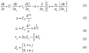
The closure coefficient (σ_k), C_d and the length scale (l) have to be specified prior to application of the equation. The values of σ_k = 1.0, C_d ranges between 0.07 and 0.09, and a mixing length similar to that of the mixing length model by Prandtl (1925), was tested by Emmons (1954), and Glushko (1965) successfully. The turbulence length scale (l) can be reasonably assumed to equal to 7% of the smallest domain calculation dimension (Fard and Boyaghchi, 2007).

Kolmogorov (1942) proposed the k-ω turbulence model. This was the first two-equation turbulence model. As did Prandtl (1945), Kolmogorov selected the turbulence kinetic energy as one of his turbulence parameters, and the second parameter (ω) represents the rate of dissipation of energy per unit of volume and time, where β and σ are the closure coefficients of the model (Eq. 7):

Wilcox (1988, 1998), Speziale et al. (1992), Peng et al. (1997), Kok (2000) and Hellsten (2005) added the production term to the Kolmogorov (k-ω) model. Wilcox (2006) represented the model in the following form:

The closure coefficients and auxiliary relations for the k-ω model:

The k-ε model was initially developed by Chou (1945), Davydov (1961) and Harlow and Nakayama (1968), and was in widespread use after Launder and Spalding (1972), and adjustment of the turbulence model closure coefficient proposed by Launder and Sharma (1974) (Eqs. 14-17).

The closure coefficient for the (k-ε) model:

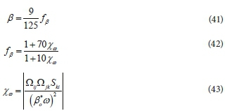
By using the renormalization group theory Yakhot and Orszag (1986), and Yakhot et al. (1992) developed the RNG k-ε model. The (C_ε٢) closure coefficient was modified by:

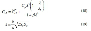
The closure coefficients for (RNG k-ε) model are:

 

METHODS

Experimental data

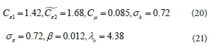
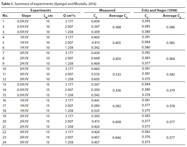
Experimental data were acquired from Aysegul and Mustafa (2016). Their experiment was conducted under steady-state conditions in a rectangular flume 8 m long, 15 cm wide, and 40 cm in height, at the Hydraulics Laboratory of the Civil Engineering Department of Dokuz Eylul University. The rate of discharge was calculated by a 90° V-notch located at the downstream part of the flume, and the flow depth was collected with a ± 0.1 mm accuracy ultrasonic level sensor (USL). The discharge ranged between 1 258 and 3 177 cm³/s due to pump capacity. Figure 2 illustrates the different parameters used in the experimental study. 24 experiments were conducted for 8 different broad-crested weir configurations (weir width B = 10 and 15 cm), and symmetrical side slopes (0.5:1, 1:1, 2:1, and 3:1) for each weir width; 3 discharges (1 258, 2 007, and 3 177 cm³/s) for each physical configuration were tested as shown in Table 1. The measured coefficient of discharge (C_D) based on the experimental results has a wide range, from 0.30 up to 0.60.

 

 

The coefficient of discharge defined by Fritz and Hager (1998) did not consider the effect of weir upstream-facing slope, as shown in Eq. 22:

Aysegul and Mustafa (2016) proposed an update to the C_D equation proposed by Fritz and Hager (1998), to take into account the effect of the approach angel (θ), as shown in Eq. 23:

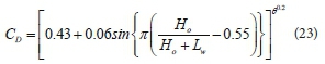
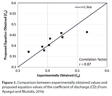
Figure 3 shows a good correlation (r = 0.87) between the proposed equation output and the experimentally obtained values for C_D.

 

 

Numerical simulations

In the present study, both three-dimensional (3-D) simulation using Flow-3D CFD package, and one-dimensional (1-D) simulation using HEC-RAS were conducted for the experimental configurations (geometric dimensions, and discharge values), as described by Aysegul and Mustafa (2016).

1-D simulations

The U.S. Army Corps of Engineers. River Analysis System (HEC-RAS version 5.0.6) is free software used to perform the one-dimensional analysis in this study. HEC-RAS simulation is based on the one-dimensional energy equation, where the friction energy loss is based on Manning's equation. In the case of rapidly varied flow the momentum equation is used (HEC-RAS 5.0.6, 2018).

24 models were simulated for the 8 different broad-crested weir configurations, and 3 discharges were used in the 3-D simulations and were similar to the experimental simulations.

The weir geometry is generated by changing the bed elevation at the weir location as shown in Fig. 4. The cross-sections are generated each 2.5 cm. The Manning coefficient (n) was selected to be 0.01 to represent the plexi-glass material of the flume. Normal depth boundary condition and known water surface boundary condition were selected at the upstream and downstream end, respectively.

 

 

3-D simulations

Flow-3D is a CFD package developed by Flow Science Incorporated of Los Alamos. Flow-3D was selected based on its capabilities in tracking free surface flow. The Flow-3D package was tested for several free surface flow problems with satisfactory outcomes (Stefan et al., 2011).

Ninety-six (96) models were simulated: 8 different broad-crested weir configurations ( weir width B = 10 and 15 cm), and symmetrical side slopes (0.5:1, 1:1, 2:1, and 3:1) for each weir width, 3 discharges (1 258, 2 007, and 3 177 cm³/s) for each physical weir configuration, and 4 turbulence models (one-equation, k-ε, RNG k-ε, and k-ω).

To avoid conflicts, the run coding is [B (weir width)-Slope (H: V)-Q (discharge)], and the legend of the turbulence model is shown on each comparison figure. Ex: 15-3:1-1258 is the run for broad-crested weir top width = 15 cm, with side slopes 3:1, and discharge 1 258 cm³/s.

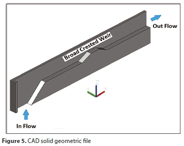
Geometric presentations and grid type

A stereolithographic (STL) file is prepared for each geometric variation in the broad-crested weir dimensions. Solid objects prepared by CAD programs are converted to STL format by approximating the solid surfaces with triangles, as shown in Fig. 5. Flow-3D uses simple rectangular orthogonal elements in planes and hexahedrals in volumes. This type of grid element eases the mesh generation, reduces the required memory resources and, due to its uniformity, enhances the numerical accuracy. The grid used is a non-adaptive grid and remains fixed throughout the calculations. The boundaries of the fluid domain in the simulation are defined by Fractional Area Volume Obstacle Representation (FAVOR), which computes the fractions of surfaces or volumes occupied by obstacles for each control volume.

 

 

Flow governing equations

The flow governing equations are three-dimensional Reynolds Averaged Naveir-Stokes equations (RANS). The equations are formulated to comply with FAVOR.

The continuity equation in Cartesian coordinates:

The momentum equations in Cartesian coordinates:

(VOF) Free surface determination

The flow free surface is a boundary with discontinuity conditions. Hirt and Nichols (1981) developed the VOF algorithm, in which a function (F) is developed to represent each grid cell occupancy with fluid. The F value varies between zero, when the grid cell contains no fluid, and unity when the grid cell is fully occupied with fluid, as shown in Fig. 6. A free surface must be in cells having F values between unity and zero. Since F is a step function, the normal direction to the cutting line represents the free surface inside the grid cell, which is perpendicular to the direction of rapid change in F values.

 

 

 

Turbulence models

In the Flow-3D package, the turbulence model equations differs slightly from other formulations to include FAVOR, and represent a slight change in the closure coefficients FLOW-3D (2010).

One-equation model

k-ε model

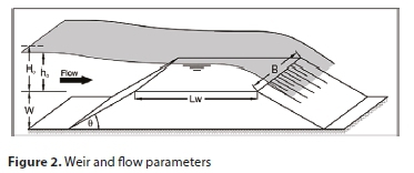
Where C1 and C2 are the closure parameters of the equation equal to 1.44 and 1.92, respectively.

RNG k-ε model

The closure factors in RNG k-ε have been changed from the normal k-ε model. C1 = 1.42, and C2 is calculated from the turbulent kinetic energy and the turbulent production terms.

k-ω model

 

Boundary conditions

To achieve accurate results, boundary conditions should be appropriately defined. Based on the measured experimental values it is clear that the flow over the broad-crested weir is a free flow, and the weir upstream generated head is not affected by the tail water conditions. In order to simulate both the head upstream of the weir, and the generated hydraulic jump at the weir downstream, the outlet boundary condition is defined as a specific pressure boundary condition type as per Flow-3D terminology, where the water level was defined as measured from the experiments. To avoid defining two parameters at the upstream end of the broad-crested weir, (head, and discharge,) the inlet configuration was simulated as the flume inlet as shown in Fig. 7, and the only defined boundary condition is the discharge from the bottom. The top boundary of the calculation domain is defined as a specific pressure boundary condition type with assigned atmospheric pressure. The bottom and sides were defined as walls.

 

 

Time step adjustment

The Courant number represents the portion of a grid cell in the direction of flow, that will be travelled by the flow during the simulation time step. Adjustable variable time step was selected to perform the CFD analyses, based on a Courant number stability criterion equal to unity.

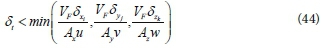
Based on the selected criteria the calculation time step varied between 0.0011 and 0.0028 seconds.

Grid generation and sensitivity analysis

Figure 8 shows the mesh generation which is one of the CFD key elements. In order to assess the adequacy of the selected mesh size for the simulation, a grid sensitivity analysis versus the parameters used in the study should be carried out. In the current study a sensitivity analysis for grid sizes 3, 2, 1, and 0.5 cm, versus 750, 1 258, 2 007, 1 258, 3 177 and 4 000 cm³/s discharges, using k-ε turbulence model, was conducted for 3 points along the weir crest, as shown in Figs 9 to 11.

 

 

 

 

 

 

 

 

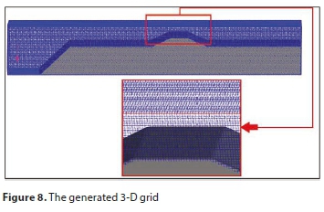
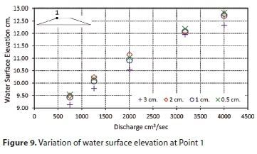
The differences between the water surface profile between mesh sizes 1 cm and 0.5 cm are negligible; accordingly a grid size of 1 cm was selected for the current study.

 

RESULTS

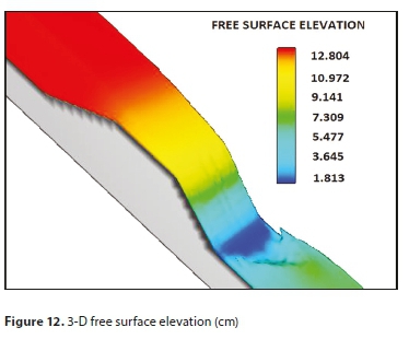
Simulation output

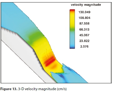
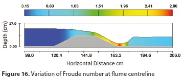
Figures 12 to 16 show a sample of the output from the 3-D simulation run No. 15-2:1-3177, using the one-equation turbulence model, while Fig. 17 shows the surface water profile obtained from the one-dimensional analysis using HEC-RAS. Figures 18-25 show the comparison between the water surface profiles obtained from each 3-D simulation using Flow-3D, and 1-D simulation using HEC-RAS, against the experimental measured values.

 

 

 

 

 

 

 

 

 

 

 

 

Analysis of results

In order to accurately assess the adequacy of each turbulence model to simulate the free surface water level (WL), mean absolute error (MAE), mean relative error percentage (RE), and root mean square error (RMSE) were calculated for each turbulence model according to the following equations:

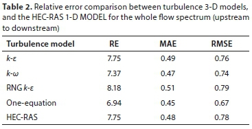
The error assessment was conducted for two zones of flow; the first is the full flow spectrum as shown in Table 2 from upstream to downstream of the broad-crested weir, and the second for the upstream part of the weir starting from the crest centerline as shown in Table 3. Figure 26 illustrates the assessment zones.

 

 

 

 

 

 

CONCLUSION

In the present study, several floodway broad-crested weirs were numerically simulated; (3-D simulation using Flow-3D CFD package, and 1-D using HEC-RAS). The Volume of Fluid (VOF) algorithm was used to define the free water surface.

Assessment of the simulation result accuracy was based on verification against the experimental results obtained for the water surface profile by Aysegul and Mustafa (2016). The relative error approach (MAE, RE, and RMSE) was utilized to check the accuracy of the simulated results.

The error assessment was conducted for two zones of flow; the first was the full flow spectrum from upstream to downstream of the broad-crested weir, and the second for the upstream part of the weir starting from the crest centerline.

The one-equation turbulence model with mixing length equal to 7% of the smallest domain dimension has the minimum error value in simulating the full spectrum free surface flow above a broad-crested weir.

For the upstream part of flow starting from the broad-crested weir centreline, no significant difference was found in accuracy between all turbulence models and the one-dimensional analysis, due to the low turbulence intensity in this section.

For engineering design purposes while the water level is the main concern at the location of the floodway the one-dimensional analysis has sufficient accuracy to define the maximum water elevation.

 

ACKNOWLEDGEMENTS

The authors would like to thank Eng. Kaleemullah Mehrabi for help in editing the text of this manuscript.

 

NOTATION

A_x, A_y, A_Z: area fraction open to flow in (x, y, and z) directions

Diff: diffusion

f_x, f_y, f_z: viscous acceleration in (x, y, and z) directions

G_x, G_y, G_z: acceleration in (x, y, and z) directions

i, j, k: unit vector in x, y, and z directions

k: kinetic energy of turbulent fluctuation per unit mass

l: turbulence length scale; a characteristic of eddy size

P: pressure

P_t: turbulence kinetic energy production

t: time

U_i: mean velocity in tensor notation

U, V, W: instantaneous velocity components in x, y, and z directions

U', V', W': fluctuating velocity components in x, y, and z directions

V_f: opened fraction volume to flow

wsx, wsy, wsz: wall shear stress in x, y, and z directions

x_i: position tensor in tensor notation

x, y, z: rectangular Cartesian coordinates

ε: dissipation per unit mass

ω: specific dissipation rate

μ: dynamic viscosity

S_ij: mean strain rate tensor

δ_ij: Kronecker delta tensor

δ_t: time step

Ω_ij: mean rotation tensor

ν: kinematic viscosity

ν_t: kinematic eddy viscosity

ν_k: kinetic energy diffusion coefficient

ν_ε: ε diffusion coefficient

ν_ω: ω diffusion coefficient

τ_ij: specific Reynolds stress tensor

λ: Taylor microscale in RNG K-e model

ρ: fluid density

 

REFERENCES

AHMED MH and MOHAMED HE (2011) Experimental and numerical investigation of flow through free double baffled gates. Water SA 37 (2) 245-254. https://doi.org/10.4314/wsa.v37i2.65871        [ Links ]

AYSEGUL OA and MUSTAFA D (2016) Experimental investigation of the approach angle effect on the discharge efficiency for broad-crested weirs. Sci. Technol. 17 (2) 279-286. https://doi.org/10.18038/btda.48930        [ Links ]

CHANSON H (2004) The Hydraulics of Open Channel Flows: An Introduction (2^nd edn). Butterworth-Heinemann, Oxford, UK. 650 pp.         [ Links ]

CHOU PY (1945) On the velocity correlations and the solution of the equations of turbulent fluctuation. Q. Appl. Math. 3 (1) 38-54.         [ Links ]

DAVYDOV BI (1961) On the statistical dynamics of an incompressible fluid. Doklady Akademiya Nauk SSSR 136 (1) 47-50.         [ Links ]

EMMONS HW (1954) Shear Flow Turbulence. In: Proceedings of the 2^nd U.S. Congress of Applied Mechanics-American Society of Mechanical Engineers, 14-18 June 1954, Michigan.         [ Links ]

FARD MH, and BOYAGHCHI FA (2007) Studies on the influence of various blade outlet angles in a centrifugal pump when handling viscous fluids. Am. J. Appl. Sci. 4 (9) 718-724. https://doi.org/10.3844/ajassp.2007.718.724        [ Links ]

FRITZ HM and HAGER WH (1998) Hydraulics of embankment weirs. Hydraul. Eng. 124 (9) 963-971. https://doi.org/10.1061/(ASCE)0733-9429(1998)124:9(963)        [ Links ]

FLOW-3D (2016), User Manual V11.2. Flow Science INK, Santa Fe.         [ Links ]

GLUSHKO G (1965) Turbulent boundary layer on a flat plate in an incompressible fluid. Izvestia Acad. Nauk. SSSR Mekh. 4 (1) 13-23.         [ Links ]

HARGREAVES DM, MORVAN HP and WRIGHT NG (2007) Validation of the volume of fluid method for free surface calculation: The broad-crested weir. Eng. Appl. Comput. Fluid Mech. 1 (2) 136-146. https://doi.org/10.1080/19942060.2007.11015188        [ Links ]

HARLOW FH and NAKAYAMA PI (1968) Transport of Turbulence Energy Decay Rate. Los Alamos Scientific Laboratory of the University of California Report LA-3854. 11 pp. https://www.osti.gov/servlets/purl/4556905        [ Links ]

HEC-RAS 5.0.6 (2018) Hydraulic reference manual. URL: https://www.hec.usace.army.mil/software/hec-ras/documentation.aspx (Accessed December 2018).         [ Links ]

HELLSTEN A (2005) New advanced k-w turbulence model for high-lift aerodynamics. AIAA 43 (9) 1857-1869. https://doi.org/10.2514/1.13754        [ Links ]

HENDERSON FM (1966) Open Channel Flow. Macmillan, New York. 522 pp.         [ Links ]

HIRT CW and NICHOLS BD (1981) Volume of Fluid (VOF) Method for the dynamics of free boundaries. Comput. Phys. 39 (1) 201-225.         [ Links ]

HOSEINI SH, JAHROMI SH, and VAHID MS (2013) Determination of discharge coefficient of rectangular broad-crested side weir in trapezoidal channel by CFD. Int. J. Hydraul. Eng. 2 (4) 64-70.         [ Links ]

HOSSEIN A and SAYED HH (2013) Experimental and 3-D numerical simulation of flow over a rectangular broad-crested weir. Int. J. Eng. Adv. Technol. 2 (6) 214-219.         [ Links ]

JIANG L, DIAO M, SUN H and REN Y (2018) Numerical modelling of flow over a rectangular broad-crested weir with a sloped upstream face. Water 10 (11) 1-12. https://doi.org/10.3390/w10111663        [ Links ]

JOONGCHEOL P and NAM JI (2015) Numerical modelling of free surface flow over a broad-crested rectangular weir. Korea Water Resour. Assoc. 48 (4) 281-290.         [ Links ]

KASSAF SI, ATTIYAH AN and YOUSIFY HA (2016) Experimental investigation of compound side weir with modelling using computational fluid dynamic. Int. J. Energ. Environ. 7 (2) 167-178.         [ Links ]

KIRKGOV MS, AKOZ MS and ONER AP (2008) Experimental investigation of compound side weir with modelling using computational fluid dynamic. Can. J. Civ. Eng. 35 (9) 975-986. https://doi.org/10.1139/L08-036        [ Links ]

KOK JC (2000) Resolving the dependence on freestream values for the k-w turbulence model. AIAA 38 (7) 1292-1295. https://doi.org/10.2514/2.1101        [ Links ]

KOLMOGOROV AN (1942) Equations of turbulent motion of an incompressible fluid. Izvestia Acad. Sci. USSR. 6 (1-2) 56-58.         [ Links ]

LAUNDER BE and SHARMA BI (1974) Application of the energy dissipation model of turbulence to the calculation of flow near a spinning disc. Lett. Heat Mass Transfer 1 (1) 131-138. https://doi.org/10.1016/0094-4548(74)90150-7        [ Links ]

LAUNDER BE and SPALDING DB (1972) Mathematical Models of Turbulence. Academic Press, London. 169 pp.         [ Links ]

MAGHSOODI R, ROOZGAR MS, SARKARDEH H and AZAMATULLA HM (2012) 3D-simulation of flow over submerged weirs. Int. J. Model. Simul. 32 (4) 237-243. https://doi.org/10.2316/Journal.205.2012.4.205-5656        [ Links ]

PENG SH, DAVIDSON L and HOLMBERG S (1997) A modified low Reynolds number k-w model for recirculating flows. Fluids Eng. 119 (4) 867-875. https://doi.org/10.1115/1.2819510        [ Links ]

PRANDTL L (1925) Uber die ausgebildete Turbulenz (About the trained turbulence). ZAMM Appl. Math. Mech. 5 (2) 136-139.         [ Links ]

PRANDTL L (1945) Uber ein neues Formelsystem fur die ausgebildete Turbulenz (About a new formula system for the deducted turbulence). In: Nachrichten Akademie der Wissenschaften in Gottingen Mathematisch-Physikalische Klasse. Springer-Verlag, Berlin.         [ Links ]

SARGISON JE and PERCY A (2009) Hydraulics of broad-crested weirs with varying side slopes. Irrig. Drain. Eng. 135 (1) 115-118. https://doi.org/10.1061/(ASCE)0733-9437(2009)135:1(115)        [ Links ]

SARKER MA and RHODES DG (2004) Calculation of free-surface profile over a rectangular broad-crested weir. Flow Meas. Instrum. 15 (4) 215-219. https://doi.org/10.1016/j.flowmeasinst.2004.02.003        [ Links ]

SHAKER AJ and SARHAN AS (2017) Performance of flow over a weir with sloped upstream face. ZNCO J. Pure Appl. Sci. 29 (3) 43-54. https://doi.org/10.21271/ZJPAS.29.3.6        [ Links ]

SHAYMAA AM, HUDA MM and THAMEEN NN (2017a) Experimental and numerical simulation of flow over broad-crested weir and stepped weir using different turbulence models. Eng. Sustainable Dev. 12 (2) 28-45.         [ Links ]

SHAYMAA AM, HUDA MM, RASUL MK, THAMEEN NN and NADHIR AA (2017b) Flow over broad-crested weirs: comparison of 2d and 3d models. Civ. Eng. Archit. 11 (1) 769-779. https://doi.org/10.17265/1934-7359/2017.08.005        [ Links ]

SHAYMAA AM, SADIQ AS and HUDA MM (2015) determination of discharge coefficient of rectangular broad-crested weir by CFD. In: Proceedings of The Second International Conference on Buildings, Construction and Environmental Engineering, 17-18 October 2015, Beirut, Lebanon.         [ Links ]

SPEZIALE CG, ABID R and ANDERSON EC (1992) Critical evaluation of two-equation models for near-wall turbulence. AIAA 3 (2) 324-331.         [ Links ]

STEFAN H, NILS RB and ROBERT F (2011) numerical modelling of flow over trapezoidal broad-crested weir. Eng. Appl. Comput. Fluid Mech. 5 (3) 397-405. https://doi.org/10.1080/19942060.2011.11015381        [ Links ]

TANASE NO, BROBOANA D and BALAN B (2015) Free surface flow over the broad-crested weir. In: Proceedings of the Ninth International Symposium on Advanced Topics in Electrical Engineering, 7-9 May 2015, Bucharest, Romania.         [ Links ]

WILCOX DC (1988) Reassessment of the scale determining equation for advanced turbulence models. AIAA 26 (11) 1299-1310. https://doi.org/10.2514/3.10041        [ Links ]

WILCOX DC (1998) Turbulence Modelling for CFD. (2^nd edn). DCW Industries, Inc., La Canada, California. 540 pp.         [ Links ]

WILCOX DC (2006) Turbulence Modelling for CFD. (3^rd edn). DCW Industries, Inc., La Canada, California. 522 pp.         [ Links ]

YAKHOT V and ORSZAG SA (1986) Renormalization group analysis of turbulence: 1. Basic theory. Sci. Comput. 1 (1) 3-51.         [ Links ]

YAKHOT V, ORSZAG SA, THANGAM S, GATSKI TB and SPEZIALE CG (1992) Development of turbulence models for shear flows by a double expansion technique. Phys. Fluids A: Fluid Dyn. 4 (7) 1510-1520. https://doi.org/10.1063/1.858424        [ Links ]

YAZDI J, SARKARDEH H, AZAMATULLA HM and GHANI AA (2010) 3D simulation of flow around a single spur dike with free surface flow. Int. J. River Basin Manag. 8 (1) 55-62. https://doi.org/10.1080/15715121003715107        [ Links ]

 

 

Received 14 April 2018
Accepted in revised form May 2019

 

 

* Corresponding author, email: Ahmed.helmi@eng.cu.edu.eg