


Services on Demand
Article
 English (pdf)
 Article in xml format
 Article references
Indicators

Related links
-
 Cited by Google
 -
 Similars in Google
Share

 Permalink
Water SA
On-line version ISSN 1816-7950
Print version ISSN 0378-4738
Water SA vol.45 n.2 Pretoria Apr. 2019
http://dx.doi.org/10.4314/wsa.v45i2.11
Assessing the accuracy of ANN, ANFIS, and MR techniques in forecasting productivity of an inclined passive solar still in a hot, arid environment
Ahmed F MashalyI, *; AA AlazbaI, II
IAlamoudi Water Research Chair, King Saud University, Riyadh, Saudi Arabia
IIAgricultural Engineering Department, King Saud University, Riyadh, Saudi Arabia
ABSTRACT
Solar still productivity (SSP) essentially describes the performance of solar still systems and is an important factor to consider in achieving a reliable design. This study presents the use of artificial neural networks (ANN), adaptive neuro-fuzzy inference systems (ANFIS), and multiple regression (MR) for forecasting the SSP of an inclined solar still in a hot, arid environment. The experimental data used for the modelling process included meteorological and operational variables. Input variables were relative humidity, solar radiation, feed flow rate, and total dissolved solids of feed and brine. The models were assessed statistically using the correlation coefficient (CC), root mean square error (RMSE), overall index of model performance (OI), mean absolute error (MAE), and mean absolute relative error (MARE). Overall, ANN was shown to be superior (CC = 0.98, RMSE = 0.05 L·m−2·h−1, OI = 0.95, MAE = 0.03 L·m−2·h−1, and MARE = 8.92%) to ANFIS and MR for SSP modelling. The relatively low errors obtained by the ANN technique led to high model predictability and feasibility of modelling the SSP. Thus, our findings indicate that ANN can be applied as an accurate method for predicting SSP.
Keywords: solar still, adaptive neuro-fuzzy inference system, artificial neural networks, multiple regression, forecasting
INTRODUCTION
A solar still is a simple device that uses solar energy to convert available brackish or saline water into fresh water for both domestic and agricultural applications. However, solar stills are not attractive in the market owing to their low productivity. Researchers worldwide have worked on the enhancement of the productivity of solar stills (Mashaly et al., 2016; Gupta et al., 2016; Rabhi et al., 2017; Panchal and Mohan, 2017). In general, experimental investigations and studies are expensive and time consuming. Therefore, some scientists and researchers have focused on mathematical modelling to find and examine important parameters and better designs for solar stills (Tiwari and Rao, 1984; Sartori, 1987; Toure and Meukam, 1997). Unfortunately, all of the above cited studies rely on mechanistic internal heat and mass transfer (HMT) models. These models typically require simplifying assumptions concerning the relative magnitude of several elements of HMT.
The large amount of data required to measure the parameters needed for evaluating and validating an HMT model limit the effectiveness of such approaches in predicting solar still productivity (SSP). Although HMT models have been used efficaciously in the past, the amount of time and data storage, and the frequency of calculations and measurements they require, might effectively make this methodology infeasible in many parts of the world today. Soft computing techniques have a potential advantage for forecasting SSP in that they require fewer parameters compared to HMT models. Soft computing is an innovative methodology for building computationally intelligent systems. Soft computing techniques can be used as alternative methods because they have advantages such as not requiring knowledge of internal system parameters, consuming less time, providing simpler solutions for multi-parameter problems and enabling factual computation (Huang et al., 2010).
As stated by Zadeh (1992), soft computing is an emerging approach towards computation that parallels the aptitude of human intelligence to understand in an environment of inaccuracy and uncertainty. Soft computing comprises artificial neural networks (ANN), genetic algorithms (GAs), fuzzy logic (FL), adaptive neuro-fuzzy inference systems (ANFIS), support vector machines (SVMs), and data mining (DM). These approaches offer advantages over conventional modelling methods, including the capability to handle large amounts of noisy data from dynamic and non-linear systems, particularly when the underlying physical processes are not fully comprehended. Many soft computing methods have been used in recent years to estimate the performance of solar-based systems, with ANFIS and ANN being the most popular. ANFIS and ANN applications have been used in estimating the performance of solar chimney power plants (Amirkhani et al., 2015), evaluating the control system for a solar-powered membrane desalination system (Porrazzo et al., 2013), calculating daily global solar radiation under sub-humid environments (Quej et al., 2017), and assessing a parabolic trough solar thermal power plant (Boukelia et al., 2017). Moreover, ANN has been used to compute thermal performance parameters of solar cookers (Kurt et al., 2008), to analyse the performance of triple solar stills (Hamdan et al., 2013), and to optimize solar still performance under a hyper-arid environment (Mashaly et al., 2015).
In this study, two different soft computing methods, ANN and ANFIS, were extended in order to estimate the productivity of an inclined solar still operating under arid conditions. The two models were implemented systematically, and in each stage the best condition with the lowest error was selected, and following that the model with highest precision, between ANN and ANFIS, was selected. To assess and confirm the effectiveness of the proposed models, they were compared with multiple regression (MR). Therefore, the present study compares the efficiency of ANN, ANFIS, and MR in the estimation of SSP using easily measurable weather and operational parameters.
MATERIALS AND METHODS
Experiment description
The experiments were conducted at the Agricultural Research and Experiment Station, Department of Agricultural Engineering, King Saud University, Riyadh, Saudi Arabia (24°44′10.90″N, 46°37′13.77″E), during the period February-April 2013, where the weather data was obtained from a weather station (model: Vantage Pro2, manufacturer: Davis, USA) located close to the experimental site (24°44′12.15″N, 46°37′14.97″E). The solar still system that was utilized in the experiments consists of one C6000 panel (F cubed. Ltd., Carocell Solar Panel, Australia). The surface area of the panel was 6 m2. This solar still is manufactured as a panel using modern cost-effective materials, such as coated polycarbonate plastic. The panel heats and distils a film of water flowing over the absorber mat of the panel. The panel was fixed at angle of 29° to the horizontal. The basic construction materials were galvanized steel legs, aluminium frame, and polycarbonate covers. The transparent polycarbonate was coated from inside with a special coating material to prevent fogging (patent for F cubed - Australia). The cross-sectional view of the solar still is presented in Fig. 1. The operational mechanism of the system is summarized in the following paragraphs.
Water was fed to the panel using a centrifugal pump (model: PKm 60, 0.5 HP, Pedrollo, Italy) with a constant flow rate of 10.74 L·h−1. Eight dripper nozzles drip the feed causing a film of water to flow over the absorbent mat. Under the absorbent mat is an aluminium screen that helps to distribute the dripping water over the absorber mat. Beneath the aluminium screen is a plate, also made of aluminium. Aluminium was selected for the manufacturing process because it is a hydrophilic material, and therefore facilitates even distribution of the sprayed water. The water flows through and over the absorbent mat, and as the solar energy is absorbed and partially collected inside the panel, the water gets heated and the resultant hot, humid air naturally circulates within the panel. The hot air flows in the upper part towards the top, and then reverses its direction towards the bottom.
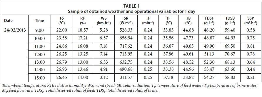
By this circulation, the humid air touches the cooled surfaces of the transparent polycarbonate cover and the bottom polycarbonate layer, due to which the water condenses and flows down the panel, and is collected as a distilled stream. Seawater was used as the feed water input to the system. Raw seawater was obtained from the Gulf, Dammam, East of Saudi Arabia (26°26'24.19" N, 50°10'20.38" E). The solar still system was run during the period 23 February 2013 to 23 April 2013. The initial concentration of the total dissolved solids (TDS), pH, density (ρ) and electrical conductivity (EC) of the raw seawater were 41.4 g∙L−1, 8.02, 1.04 g·cm−3, and 66.34 mS·cm−1, respectively. The productivity or the amount of distilled water produced (SSP) for a given time period by the system was obtained by collecting the cumulative amount of water produced over the time period. The temperatures of the feed (TF) and brine (TB) were measured using thermocouples (T-type, UK). Temperature data for the feed brine water were recorded on a data logger (model: 177-T4, Testo, Inc., UK) at 1 min intervals. The amount of feed water (MF) was measured by a calibrated digital flow meter (Micro-Flo, Blue-White, USA) that was mounted on the feed water line. The amount of brine water and distilled water were measured by a graduated cylinder. TDS and EC were checked using a calibrated (TDS) meter (Cole-Parmer Instrument, Vernon Hills, USA). A pH meter (model: 3510 pH meter, Jenway, UK) was utilized to determine the pH. ρ was measured by a digital density meter (model: DMA 35N, Anton Paar, USA). The seawater was fed separately to the panel using the pump mentioned above. The transit time for the water to pass through the panel was about 20 min. Consequently, the flow rate of the feed water, distilled water and brine water were measured every 20 min. In addition, the total dissolved solids in the feed water (TDSF) and brine water (TDSB) were measured every 20 min. Weather data such as ambient temperature (To), relative humidity (RH), wind speed (WS), and solar radiation (SR) were obtained from the weather station mentioned above. Overall, we have 1 dependent variable, SSP, and 9 independent variables, which are To, RH, WS, SR, TF, TB, TDSB, TDSF, and MF. A sample of the meteorological and operational data is presented in Table 1. Summary statistics of the available experimental data are presented in Table 2.
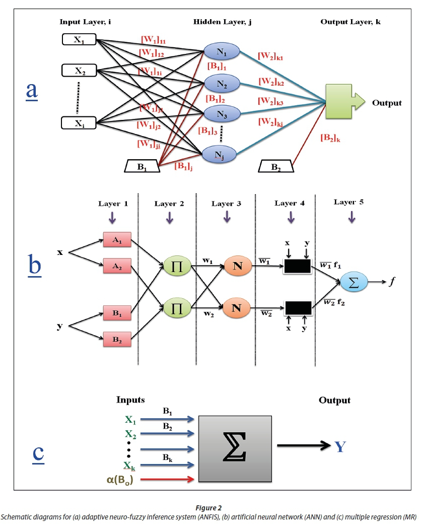
Artificial neural networks (ANNs)
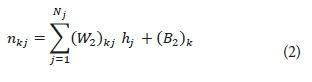
ANNs are computational modelling tools that attempt to simulate structures or functions inspired by biological neural networks. In this study, the feed-forward back propagation algorithm (FFBPA) is used for the ANN model. The FFBPA neural network is the most popular and widely used ANN architecture (Rumelhart et al., 1986). It consists of one input layer, one or more hidden layers and one output layer. The ANN architecture used for this study is demonstrated in Fig. 2. The input layer (i) is connected to the hidden layer (j), which is in turn linked to the output layer (k) through the connection weights (W) and biases (B). The weights are used to change the parameters of the throughput and the varying connections to the neurons (n). The biases are connected to all neurons in the hidden and output layers and used to maintain the universal approximation of the ANN. A neuron (processing element) comprises of 2 parts in the hidden layer. The first part aggregates the weighted inputs adding up to a quantity 1. The second part is the transfer/activation function that assists the translation of the input parameters (the activation values of the nodes) into the desired output parameter. The precise mathematical expression and explanation of the ANN are as follows (Haykin, 1999): The output layer neuron (Yk) can be expressed as follows:

where nkj is the input to the k-th output neuron and can be estimated using the formula:
Therefore:

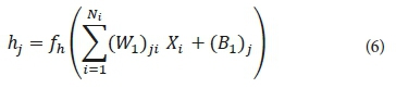
Further, the neuron's activation value (hj) in the hidden layer is mathematically expressed using the following formula:

where nji is the input of the j-th neuron in the hidden layer, which is calculated from:

Accordingly, the hj can be written as:
By substituting Eq. 10 in Eq. 6, Yk can be calculated as follows:

With rearrangement, Eq. 15 might be written as:
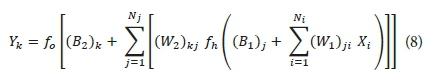
where Xi are input parameters; Ni is the number of input neurons; Nj is the number of output neurons; (W1)ji are the weights from the input layer to the hidden layer; (W2)kj are the weights from the hidden layer to the output layer; (B1)j are the biases in the hidden layer; (B2)k are the biases in the output layer; fh is the activation (transfer) function in the hidden layer; and fo is the activation function in the output layer.
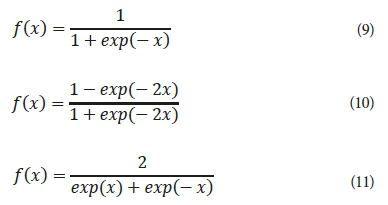
In this study, we employed 3 different types of activation functions: sigmoid, hyperbolic tangent, and hyperbolic secant in each of the hidden and output layers to train the ANN. The general functional forms of the sigmoid (SIGM) (Eq. 9), hyperbolic tangent (TANH) (Eq. 10), and hyperbolic secant (SECH) (Eq. 11) transfer functions can be expressed as:
The ANN model was developed using the Qnet2000 software. In this study, the available data obtained from the experimental work were randomly divided into 3 portions: 70% as the training datasets (112 data points) for the learning process, 20% as the testing datasets (32 data points) to test the precision of the model and 10% for the validation procedure (16 data points).
Before the modelling process, the data is automatically normalized between 0.15 and 0.85. The normalization accelerates the training process, and enhances the network's generalization capabilities. However, to avoid over-training, the number of iterations was limited and fixed to 10 000. Increasing the epoch size may worsen the problem of over-training. The learn rate and momentum factor were fixed at 0.01 and 0.8, respectively. Different ANN architectures with one hidden layer were trained. The optimal number of neurons in the hidden layer was determined by a trial and error procedure, where the number of neurons in the hidden layer was varied from 2 to 20. However, the number of the neurons should not be set to too high a number, to avoid over-training, or set to too low a number, which can lead to insufficient generalization. In addition, the transfer function was varied between SIGM, TANH, and SECH in the hidden and output layers, in order to find the best transfer function among them. These procedures mentioned above enable us to find the best architecture for the ANN model.
The training process for the FFBPA neural network is carried out repetitively, until the error between the desired value and the forecasted value becomes minimal, and the training process moves towards stabilization. The ideal structure for this neural network is 3 layers: one for each of the input, hidden, and output layers. Only one hidden layer is required in FFBPA, because a 3-layer network can produce arbitrarily complex decision regions (Maier and Dandy, 2000). The increasing technique was used for selecting the number of neurons for evaluation of various configurations. In this technique, when the ANN reaches a local minimum, new neurons are added to the ANN gradually. This technique has greater practical utility than other techniques typically used for detecting the optimum size of an ANN. The advantage of this method is that the ANN complexity improves gradually with the increase in neurons. The optimum size of the ANN is always obtained by adjustments. Monitoring and assessing the local minimum is done during the training process. These procedures help to avoid local minima convergence and overtraining, increase the predictive ability of a network, and remove spurious effects caused by random starting values.
Adaptive neuro-fuzzy inference system (ANFIS)
The adaptive neuro-fuzzy inference system (ANFIS), which incorporates the best features of fuzzy logic (FL) and artificial neural network (ANN) systems, is defined by Jang (1993). As an architecture, the ANFIS is composed of if-else rules and input-output data couples of fuzzy logic, and it uses learning algorithms from neural networks for training. Moreover, ANFIS is an approach to simulate complex nonlinear mappings using neural network learning and fuzzy inference methodologies, and has the capability of working with uncertain, noisy and inaccurate environments. ANFIS utilizes the ANN training process to adjust the membership function and the associated parameter that approaches the desired datasets. The learning algorithm in ANFIS is a hybrid learning algorithm that utilizes the back-propagation learning algorithm and least squares method together. In order to understand and simplify the process, a sample having 2 inputs and an output is considered. Five layers are used to build an ANFIS architecture of the first-order Sugeno-type inference system presented in Fig. 2. Two inputs, x and y, and one output, f, along with two fuzzy IF-THEN rules are taken into account as an example. In Fig. 2, the circle and square show a fixed node and an adaptive node, respectively. The functions of each of the 5 layers are explained in the following sections. For a first-order Sugeno fuzzy model, the following two fuzzy if-then rules are used (Jang, 1993):

where x and y are the inputs and A1, B1, A2, B2 are fuzzy sets, p1, p2, q1, q2, r1, and r2 are the coefficients of the output function that are determined during the training.
Layer 1 is the fuzzification layer (layer of input nodes). Every node i is an adaptive node with a node output expressed by:
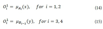
where µAi and µBi-2 are the fuzzy membership functions.
Layer 2 is the rule layer (layer of rule nodes). Every node i in this layer is a fixed node, marked by a circle and labelled Π, representing simple multiplication. The output of this layer is the product of all the incoming signals and can be formulated as:

Layer 3 is the normalization layer (layer of average nodes). In this layer, the ith node is a circle labelled N, and computes the normalized firing strength as follows:

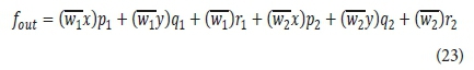
Layer 4 is the defuzzification layer (layer of consequent nodes). In this layer, every node i marked by a square is an adaptive node with a node function. The output of this layer is calculated by:

where {pi, qi, ri} is the parameter set of this node.
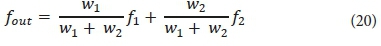
Layer 5 is the output layer. The single node in this layer is a fixed circle node labeled ∑, which calculates the final overall output as the summation of all incoming signals. The overall output is computed by this formula:

Finally, the overall output can be formulated as:
Substituting Eq. 7 into Eq. 10:

The final output can be written as:
As in the ANN modelling, the ANFIS modelling process includes 3 stages: training, testing and validation. The data division is the same as that used with ANN modelling. Therefore, the training, testing, and validation sets have 112, 32, and 16 data points, respectively. Before training, the data are normalized to be in the range between 0 and +1 in order to decrease their range and increase the precision of the findings. After the normalization process, the data are ready for the training process.
The MATLAB software (MATLAB 8.1.0.604, R2013a, the MathWorks Inc., USA) was used to develop the ANFIS model from the experimental data to forecast SSP. The Sugeno-type fuzzy inference system was used in the modelling of SSP. The grid partition method was employed to classify the input data and in making the rules (Jang, 1993). In the modelling process, we employed 8 different types of input MFs, including triangle (TRIMF), trapezoidal (TRAPMF), generalized bell (GBELLMF), Gaussian (GAUSSMF), 2-sided Gaussian (GASUSS2MF), Pi curve (PIMF), product of 2 sigmoidal functions (PSIGMF), and difference between 2 sigmoidal functions (DSIGMF). The output MF was selected as a linear function. Moreover, a hybrid learning algorithm that combines the least-squares estimator and the gradient descent method was utilized to estimate the optimum values of the FIS parameters of the Sugeno-type inference system (Jang, 1993). The number of epochs was chosen as 50 owing to their small error.
Multiple regression (MR)
Linear regression is the oldest statistical method in regression and can be considered a benchmark for new methods. Multiple regression (MR) is a linear statistical method that attempts to find the best relationship between a dependent parameter and several other independent parameters through the least square method and by fitting a linear equation to the observed data. Every value of the independent parameter x is associated with a value of the dependent parameter y. The MR model can be formulated as follows:

where Y is the dependent parameter or response, k is the number of independent parameters, Xj is the independent parameter, β is the regression coefficient, j = 0, 1, 2,…,k, and ε is a term that contains the influences of un-modeled sources of variability that impact the dependent parameter.
The functional connection between the dependent and independent parameters can be expressed in matrix form as follows:

where Y is an output parameter vector of size n × 1; X is an input parameter matrix of size n × (p + 1); β is a coefficient vector of size (p + 1) × 1 and e is an error vector of size n × 1. According to Eq. 9, p multi-linear regressions can be expressed as follows:

β regression parameter coefficients in matrix form can be illustrated as follows:

where β regression coefficients are found through the least square technique; (X′X)-1 is the inverse of the X′X matrix, and X′ is the transpose of the X matrix.
A schematic diagram of the MR process is described in Fig. 2. It is important to assess the goodness-of-fit and the statistical significance of the estimated parameters of the developed regression models; the procedures that are usually applied to verify the goodness-of-fit of regression models are hypothesis testing, R2 and the analysis of residuals. For this purpose, the F-test is used to verify the statistical significance of the overall fit and the t-test is used to assess the significance of the individual parameters. In other words, the t-test examines the importance of individual coefficients, while the F-test is utilized to compare different models to assess the model that best fits the population of the sample data (Um et al., 2011). In this study, the SPSS software (IBM Inc., USA) was used to develop the MR model. The same data used for developing the ANN and ANFIS models were used in the development of the MR model.
ANN, ANFIS, and MR model performance assessment criteria
The performance of the ANFIS and ANN models were assessed based on the coefficient of correlation (CC), the root mean square error (RMSE), the overall index of model performance (OI), the mean absolute error (MAE), and the mean absolute relative error (MARE). These indicators can be mathematically described and computed through Eqs. (14)-(18) (Mashaly and Alazba, 2016).
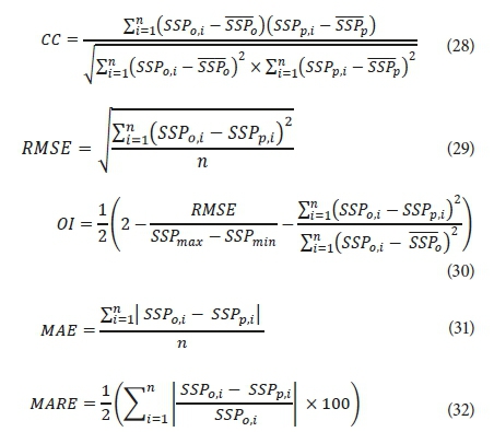
where n is the number of data points, SSPo,iand SSPp,i are the observed and predicted values respectively,  and
and  are the means of the observed and predicted values respectively, and SSP max and SSPmin are the maximum and minimum measured values, respectively.
RESULTS AND DISCUSSION
Data description and variable selection
Table 2 shows the statistical summary of the experimental data (To, RH, WS, SR, TF, TB, TDSB, TDSF, MF, and SSP). This table summarizes statistical details about these parameters such as the maximum, minimum, mean, standard error, median, standard deviation, kurtosis, skewness, and coefficient of variation for each parameter. From Table 2, it is seen that the distribution curves for To, RH, SR, TF, TB, MF, TDSF, TDSB, and SSP are platykurtic since the kurtosis values are less than 3. On the other hand, the distribution curve for WS is leptokurtic as the kurtosis value is greater than 3. The distributions are highly skewed for RH and WS because the skewness values are greater than +1. The skewness values for SR, TF, and MF are between −1 and −1/2 and, therefore, the distributions for these variables are moderately skewed. Moreover, the distributions are approximately symmetric for To, TB, TDSF, TDSB, and SSP since the skewness values are between −1/2 and +1/2. From the coefficient of variation (CV) values, it is clear that the data for To, TF and TB are relatively homogenous (0.10 ≤ CV< 0.20). In addition, the data for MF is relatively heterogeneous (0.20 ≤ CV< 0.30). Finally, the data for RH, WS, SR, TDSF, TDSB, and SSP are heterogeneous (CV ≥ 0.30).
Parameter selection is the process of selecting an optimum subset of input parameters from the set of potentially useful parameters that may be available in the context of a given problem. In this study, we adopt stepwise regression to analyse and select parameters, which consequently increases the predictive accuracy of the developed models. A stepwise regression technique (i.e., step-by-step iterative construction of a regression model that includes automatic selection of independent parameters) was applied to explore relationships among the collected data. The Mallows statistic (Cp) was employed as a criterion to select the set of independent factors that most closely determines the dependent parameter. Cp is a powerful selection procedure in a stepwise analysis. The purpose of Cp is to guide the researcher in the process of subset selection. Good subsets are ones with small Cp values and/or values of Cp close to the number X of variables in the model (Mallows, 1995; Kadane and Lazar, 2004). The result of the stepwise analysis according to the Cp coefficient is presented in Table 3. According to results presented in Table 3, the model with the 5 terms 'RH, WS, SR, TDSF, and TDSB' is relatively precise and unbiased because its Mallows' Cp (5.029) is small and closest to the number of variables plus the constant (6). Therefore, the ANN, ANFIS, and MR models were trained using these variables.

ANN model
To determine the best ANN architecture to use, we varied the number of neurons/nodes in the hidden layer. In addition, the transfer/activation function was varied between the sigmoid (SIGM), hyperbolic tangent (TANH), and hyperbolic secant (SECH) functions in the hidden and output layers. Table 4 displays the results of the statistical performance of the ANN models with various neuron numbers in the hidden layer and various transfer functions during the training process. The number of nodes in the hidden layer, along with the identification of activation functions between the layers, was determined through a trial-and-error procedure to select the best ANN model architecture. The number of neurons was increased from 2 to 20 in the hidden layer.
We examined the CC, RMSE, OI, MAE, and MARE values as the number of hidden neurons in the ANN was increased. Generally, the ANN architecture markedly improved with higher numbers of hidden neurons, as reflected in the values of the statistical indicators for the three activation functions (Table 4). The ANN-SIGM models' CC values ranged from 0.983 to 0.992, RMSE values from 0.030 to 0.044 L·m−2·h−1, OI values from 0.960 to 0.976, MAE values from 0.020 to 0.033, and MARE values from 5.259 to 8.221. The ANN-TANH models' CC values ranged from 0.983 to 0.992, RMSE values from 0.030 to 0.044 L·m−2·h−1, OI values from 0.960 to 0.976, MAE values from 0.019 to 0.032, and MARE values from 5.031 to 7.960. Furthermore, the ANN-SECH models' CC values ranged from 0.983 to 0.992, RMSE values from 0.030 to 0.044 L·m−2·h−1, OI values from 0.960 to 0.976, MAE values from 0.018 to 0.032, and MARE values from 4.759 to 8.595. Clearly, the SECH function is more accurate than the SIGM and SECH functions.
As illustrated in Table 4, the SECH function performed better than the SIGM and TANH functions, and there was an obvious enhancement in the model when the number of hidden nodes was increased, especially when the SECH function was used. This is in accordance with Boroomand-Nasab and Joorabian (2011) and Kamanbedast (2012). High values of CC and OI, and low values of RMSE, MAE and MARE, indicating good model performance, were obtained by increasing the number of neurons in the hidden layer. The SECH function yielded the best network performance for SSP. When the number of hidden neurons reached 10, there was a clear improvement in the ANN when the SECH function was used. From Table 4, it can be seen that the best architecture of the ANN model has 10 neurons in the hidden layer. The CC, RMSE, OI, MAE, and MARE for this configuration are marked in bold in Table 4, and are 0.994, 0.028 L·m−2·h−1, 0.979, 0.019, and 4.964, respectively.
However, the ANN model with one hidden layer and 10 neurons in the hidden layer was selected as the optimum ANN model for predicting SSP. The transfer function for this model was SECH for the hidden and output layers. This function yielded the best network performance and generally performed better than the SIGM and TANH, as shown in Table 4. Therefore, the developed ANN model architecture has a configuration of 5-10-1 neurons. This yielded the best prediction of SSP with the lowest error.
ANFIS model
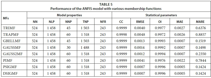
This section discusses the 8 ANFIS models developed during the training process, with additional details about the best ANFIS model. We developed 8 ANFIS models with 8 different types of input membership functions (MFs). The MFs used were TRIMF, TRAPMF, GBELLMF, GAUSSMF, GASUSS2MF, PIMF, DSIGMF, and PSIGMF. The ANFIS models developed have 5 inputs (RH, SR, MF, TDSF, and TDSB) and one output (SSP). Table 5 shows the outcomes of the statistical parameters, CC, RMSE, OI, MAE, and MARE, which are numerical indicators used to assess the agreement between the observed and predicted SSP values during the training stage.
For all the ANFIS models, in the input layer, 5 neurons were incorporated. For each of the neurons, 3 identical MFs were considered with 3 linguistic terms (low, medium, high) and accordingly 243 (3 × 3 × 3 × 3 × 3) rules were developed for the implementation of the ANFIS model. The model properties of the ANFIS model structures are listed in Table 5. The ANFIS models' CC values ranged from 0.9998 to 0.9999, RMSE values from 0.0007 to 0.0048 L·m−2·h−1, OI values from 0.9972 to 0.9996, MAE values from 0.0005 to 0.0027 L·m−2·h−1, and MARE values from 0.1424 to 0.8857%. The CC and OI values are very close to 1 while RMSE, MAE, and MARE values are close to zero, indicating excellent agreement between the measured results and the predicted results in the ANFIS models during the training stage. These findings emphasize the accuracy and efficiency of the ANFIS models for estimating SSP by using the 8 MFs.
The performances for all MFs at the training stage are approximately the same. However, in relative terms, the highest performance in the training process is obtained with GBELLMF. The CC, RMSE, OI, MAE, and MARE for GBELLMF were 0.9999, 0.0013 L·m−2·h−1, 0.9993, 0.0007 L·m−2·h−1 and 0.1519%, respectively. This agrees with the results of Taghavifar and Mardani (2014) and Xie et al. (2017). However, the best ANFIS structure for SSP prediction was obtained by using GBELLMF which consisted of 5 layers and is marked in bold in Table 5. Therefore, this ANFIS structure was selected. The 1st layer of the developed model included the input parameter (RH, SR, MF, TDSF, and TDSB) membership functions (MFs). This layer provides the input parameter values to the following layer. The 2nd layer, which was an MF layer, determined and checked the weights for each MF. For the best ANFIS model, the fuzzification layer (2nd layer) contained 15 nodes and 45 non-linear parameters. The rule layer (3rd layer) with 524 nodes achieved a pre-condition matching process for fuzzy rules. The 4th layer (the defuzzification layer) with 524 nodes and 1 458 linear parameters took the inference of the rules and generated output values. The 5th layer summed up and combined the inputs and transformed the fuzzy classification into a binary outcome. Overall, the total number of parameters and fuzzy rules were 1 503 and 243, respectively, for the ANFIS model using GBELLMF.
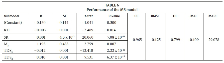
MR model
In this study, the MR model was selected to develop a relationship between the SSP and the 5 variables that affect it (RH, SR, MF, TDSF, and TDSB). The SSP was the dependent variable, while the other variables were independent. The following mathematical expression was obtained to estimate SSP based on MR analysis:
B, SE, t-stat, and the p-value of independent parameters have been listed in Table 6.
SR is an influential parameter in the computation of SSP, since the SE of the coefficients of this parameter is ± 4.3 10-05. All the values of t-stat for independent parameters are greater than +1.983 or less than −1.983, confirming the goodness of the coefficients. The absolute value of these t-stat values should be greater than 1.983 (critical t-value at 106 degrees of freedom) to ensure the goodness of the coefficients. The values of the regression coefficients for all parameters were highly and statistically significant (P-value < 0.05). However, SR is the most significant parameter in the MR model with the highest t-stat (20.060). In addition, it is revealed that the RH and TDSF were inversely proportional to SSP. The statistical parameters of the multiple regression tabulated in Table 6 were calculated using the learning/training process. The CC, RMSE, OI, MAE and MARE obtained were 0.965, 0.125 L·m−2·h−1, 0.799, 0.109 L·m−2·h−1, and 29.078%, respectively.
Comparison of models
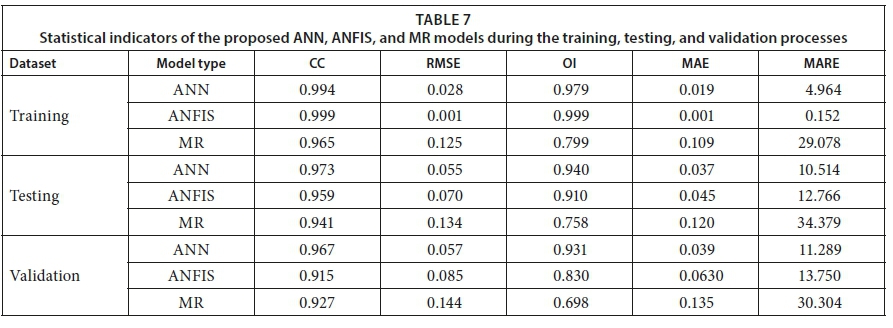
In this section, we compare the performances between the ANN model, ANFIS model, and the MR model. The performances of these models were assessed according to statistical criteria such as CC, RMSE, OI, MAE, and MARE. The findings based on applying these models are compared in Table 7. During the training process, it is clear from Table 7 that the values predicted by the ANN fit almost perfectly with the observed values, but a little less closely than those predicted by the ANFIS model, as reflected in the values of the statistical indicators. These results indicate that the ANN model is better than the MR model in the training process.
During the testing process, the CC values for the ANFIS and MR models were about 1.44% and 3.29%, respectively, and less accurate than that of the ANN model, as shown in Table 7. The RMSE values for the ANFIS and MR models were about 1.27 and 2.44 times higher, respectively, than the value for the ANN model. The OI values for the ANFIS and MR models are less than that for the ANN model. The values of MAE for the ANFIS and MR models (0.045 L·m−2·h−1and 0.120 L·m−2·h−1) were almost 1.22 and 3.24 times that of the ANN model. In addition, the values of MARE for the ANFIS and MR models were nearly 1.21 and 3.27 times that of the ANN model. During the validation process, the ANFIS and MR models had CC values of about 5.38% and 4.14%, respectively, and these were less accurate than that of the ANN model, as indicated in Table 7. The values of RMSE for the ANFIS and MR models (0.085 L·m−2·h−1and 0.144 L·m−2·h−1, respectively) were almost 1.49 and 2.53 times that of the ANN model (0.057 L·m−2·h−1). The OI value for the ANN model was 10.85% and 25.03% more accurate than that of the ANFIS and MR models, respectively. The MAE values of 0.063 L·m−2·h−1 and 0.135 L·m−2·h−1for the ANFIS and MR models were larger by 61.54% and 246.15%, respectively, than that of the ANN model. The MARE value in the ANN model was 21.80% and 168.44% less than that for the ANFIS and MR models, respectively. The CC, RMSE, OI, MAE, and MARE values confirm that the ANFIS and MR models perform relatively poorly. Table 7 clearly reveals that the predictive performance of the ANN model are significantly higher than those of the ANFIS and MR models. These outcomes indicate that the ANN model can be used successfully for SSP modelling.
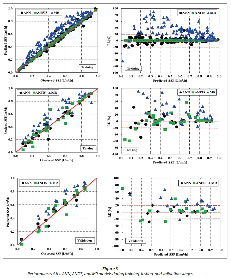
Another representation of the findings generated using the developed models is demonstrated in Fig. 3, where the scatter plots and relative errors (REs) show the accuracy of the models in predicting the SSP. In addition, the comparison of the measured and estimated data obtained from ANN, ANFIS, and MR models is presented in Fig. 3, which clearly shows that the ANN model fits more perfectly than the ANFIS and MR models. The data were mostly evenly distributed around the 1:1 line, showing a very close visual agreement between the observed and predicted values for the ANN model. Further, Fig. 3 shows the REs of predicted SSP values for the training, testing, and validation datasets for the ANN, ANFIS, and MR models. This figure shows differences between the results of the two models with average relative errors of 0.01%,−1.12%, and 6.23% for the ANFIS model when using the training, testing, and validation datasets, respectively. The figure also shows the average relative errors of 25.39%, 32.84%, and 27.65% for the MR model when using the training, testing, and validation datasets, respectively. The corresponding values for the ANN model were generally lower at 0.22%, 0.31%, and 5.41% for the training, testing, and validation datasets, respectively. In general, Fig. 3 and Table 7 convincingly demonstrate the superiority of ANN to ANFIS and MR. This is in agreement with findings of previous studies (Choubin et al., 2016; Khademi et al., 2016).
CONCLUSIONS
In this investigation, we discussed the use of artificial neural network (ANN), adaptive neuro-fuzzy inference system (ANFIS), and multiple regression (MR) for SSP modelling, acquired experimental data from a passive inclined solar still in an arid climate, and applied the above models to this data. Further, since input selection is a significant step in modelling, we used a stepwise technique to arrive at 5 combinations. Based on the outcomes of the stepwise analysis, 5 parameters, RH, SR, MF, TDSF, and TDSB, were used as input parameters. The only output parameter is the SSP. In order to evaluate the performance of the ANN, ANFIS, and MR models, 70%, 20%, and 10% of the experimental data were utilized for model training, testing, and validating, respectively. The predicted SSP values were compared to the observed values, where the assessment was based on the statistical error indicators CC, RMSE, OI, MAE, and MARE. The findings show that the ANN, ANFIS, and MR models can estimate SSP successfully and accurately. However, the ANN model performs better than the ANFIS and MR models. In particular, an ANN model with architecture 5-10-1, trained using the back-propagation algorithm and with a hyperbolic secant activation function in the hidden and output layers, is found to be the optimal model for predicting SSP.
ACKNOWLEDGEMENT
The project was financially supported by King Saud University, Vice Deanship of Research Chairs.
REFERENCES
AMIRKHANI S, NASIRIVATAN SH, KASAEIAN AB and HAJINEZHAD A (2015) ANN and ANFIS models to predict the performance of solar chimney power plants. Renew. Energ. 83 597-607. https://doi.org/10.1016/j.renene.2015.04.072 [ Links ]
BOROOMAND-NASAB B and JOORABIAN M (2011) Estimating monthly evaporation using artificial neural networks. J. Environ. Sci. Eng. 5 88-91. [ Links ]
BOUKELIA TE, ARSLAN O and MECIBAH MS (2017) Potential assessment of a parabolic trough solar thermal power plant considering hourly analysis ANN-based approach. Renew. Energ. 105 324-333. https://doi.org/10.1016/j.renene.2016.12.081 [ Links ]
HAMDAN MA, HAJ KHALIL RA and ABDELHAFEZ EAM (2013) Comparison of neural network models in the estimation of the performance of solar still under Jordanian climate. J. Clean Energ. Technol. 1 (3) 238-242. [ Links ]
HAYKIN S (1999) Neural Networks. A Comprehensive Foundation. Prentice Hall International Inc., New Jersey. [ Links ]
HUANG Y, LAN Y, THOMSON SJ, FANG A, HOFFMANN WC and LACEY RE (2010) Development of soft computing and applications in agricultural and biological engineering. Comput. Electron. Agric. 71 (2) 107-127. https://doi.org/10.1016/j.compag.2010.01.001 [ Links ]
JANG J (1993) ANFIS: adaptive-network-based fuzzy inference system. IEEE Trans. Syst. Man. Cybern. 23 665-685. https://doi.org/10.1109/21.256541 [ Links ]
KADANE JB and LAZAR NA (2004) Methods and criteria for model selection. Am. Stat. Assoc. 99 279-290. https://doi.org/10.1198/016214504000000269 [ Links ]
KAMANBEDAST AA (2012) The investigation of discharge coefficient for the Morning Glory Spillway using artificial neural network. World Appl. Sci. J. 17 (7) 913-918. [ Links ]
KHADEMI F, JAMAL SM, DESHPANDE N and LONDHE S (2016) Predicting strength of recycled aggregate concrete using artificial neural network, adaptive neuro-fuzzy inference system and multiple linear regression. Int. J. Sust. Built Environ. 5 (2) 355-369. https://doi.org/10.1016/j.ijsbe.2016.09.003 [ Links ]
KURT H, ATIK K, ÖZKAYMAK M and RECEBLI Z (2008) Thermal performance parameters estimation of hot box type solar cooker by using artificial neural network. Int. J. Therm. Sci. 47 (2) 192-200. https://doi.org/10.1016/j.ijthermalsci.2007.02.007 [ Links ]
MAIER HR and DANDY GC (2000) Neural networks for the prediction and forecasting of water resources variables: a review of modeling issues and application. Environ. Model. Softw. 15 (1) 101-124. https://doi.org/10.1016/S1364-8152(99)00007-9 [ Links ]
MALLOWS CL (1995) More comments on Cp. Technometrics 37 362-372. [ Links ]
MASHALY AF and ALAZBA AA (2016) Comparison of ANN, MVR, and SWR models for computing thermal efficiency of a solar still. Int. J. Green Energ. 13 (10) 1016-1025. https://doi.org/10.1080/15435075.2016.1206000 [ Links ]
MASHALY AF, ALAZBA AA and AL-AWAADH AM (2016) Assessing the performance of solar desalination system to approach near-ZLD under hyper arid environment. Desalin. Water Treat. 57 (26) 12019-12036. https://doi.org/10.1080/19443994.2015.1048738 [ Links ]
MASHALY AF, ALAZBA AA, AL-AWAADH AM and MATTAR MA (2015) Predictive model for assessing and optimizing solar still performance using artificial neural network under hyper arid environment. Sol. Energy 118 41-58. https://doi.org/10.1016/j.solener.2015.05.013 [ Links ]
PANCHAL H and MOHAN I (2017) Various methods applied to solar still for enhancement of distillate output. Desalination 415 76-89. https://doi.org/10.1016/j.desal.2017.04.015 [ Links ]
PORRAZZO R, CIPOLLINA A, GALLUZZO M and MICALE G (2013) A neural network-based optimizing control system for a seawater-desalination solar-powered membrane distillation unit. Comput. Chem. Eng. 54 79-96. https://doi.org/10.1016/j.compchemeng.2013.03.015 [ Links ]
QUEJ VH, ALMOROX J, ARNALDO JA and SAITO L (2017) ANFIS, SVM and ANN soft-computing techniques to estimate daily global solar radiation in a warm sub-humid environment. J. Atmos. Sol-Terr. Phys. 155 62-70. https://doi.org/10.1016/j.jastp.2017.02.002 [ Links ]
RABHI K, NCIRI R, NASRI F, ALI C and BACHA HB (2017) Experimental performance analysis of a modified single-basin single-slope solar still with pin fins absorber and condenser. Desalination 416 86-93. https://doi.org/10.1016/j.desal.2017.04.023 [ Links ]
RUMELHART DE, HINTON GE and WILLIAMS RJ (1986) Learning representations by back propagating errors. Nature 323 533-536. https://doi.org/10.1038/323533a0 [ Links ]
SARTORI E (1987) On the nocturnal production of a conventional solar still using solar pre-heated water. Proc. ISES Solar World Congr., Hamburg, Germany, pp. 1427-1431. [ Links ]
TAGHAVIFAR H and MARDANI A (2014) On the modeling of energy efficiency indices of agricultural tractor driving wheels applying adaptive neuro-fuzzy inference system. J. Terramechanics 56 37−47. https://doi.org/10.1016/j.jterra.2014.08.002 [ Links ]
TIWARI GN and RAO VSVB (1984) Transient performance of single basin solar still with water flowing over the glass cover. Desalination 49 231-241. https://doi.org/10.1016/0011-9164(84)85035-3 [ Links ]
TOURE S and MEUKAM P (1997) A numerical model and experimental investigation for a solar still in climactic conditions in Abidjan (Côte d'Ivoire). J. Renew. Energ. 11 319-330. https://doi.org/10.1016/S0960-1481(96)00131-0 [ Links ]
UM MJ, YUN H, JEONG CS and HEO JH (2011) Factor analysis and multiple regression between topography and precipitation on Jeju Island, Korea. J. Hydrol. 410 (3-4) 189-203. https://doi.org/10.1016/j.jhydrol.2011.09.016 [ Links ]
XIE Q, NI JQ and SU Z (2017) A prediction model of ammonia emission from a fattening pig room based on the indoor concentration using adaptive neuro fuzzy inference system. J. Hazardous Mater. 325 301-309. https://doi.org/10.1016/j.jhazmat.2016.12.010 [ Links ]
ZADEH LA (1992) Fuzzy logic, neural networks and soft computing. One-page course announcement of CS 294-4, University of California at Berkeley. [ Links ]
Received 15 December 2017
Accepted in revised form 11 March 2019
* To whom all correspondence should be addressed. e-mail:amashaly@ksu.edu.sa or mashaly.ahmed@gmail.com

