


Servicios Personalizados
Articulo
 Inglés (pdf)
 Articulo en XML
 Referencias del artículo
Indicadores

Links relacionados
-
 Citado por Google
 -
 Similares en Google
Compartir

 Permalink
Water SA
versión On-line ISSN 1816-7950
versión impresa ISSN 0378-4738
Water SA vol.45 no.2 Pretoria abr. 2019
http://dx.doi.org/10.4314/wsa.v45i2.05
Assessment of probable causes of chlorine decay in water distribution systems of Gaborone city, Botswana
Denis NonoI, *; Phillimon T OdirileI; Innocent BasupiII; Bhagabat P ParidaI
IDepartment of Civil Engineering, University of Botswana, Private Bag 0061, Gaborone, Botswana
IIBotswana Institute for Technology Research and Innovation, Private Bag 0082, Gaborone, Botswana
ABSTRACT
Gaborone city water distribution system (GCWDS) is rapidly expanding and has been faced with the major problems of high water losses due to leakage, water shortages due to drought and inadequate chlorine residuals at remote areas of the network. This study investigated the probable causes of chlorine decay, due to pipe wall conditions and distribution system water quality in the GCWDS. An experimental approach, which applied a pipe-loop network model to estimate biofilm growth and chlorine reaction rate constants, was used to analyse pipe wall chlorine decay. Also, effects of key water quality parameters on chlorine decay were analysed. The water quality parameters considered were: natural organic matter (measured by total organic carbon, TOC; dissolved organic carbon, DOC; and ultraviolet absorbance at wavelength 254, UVA-254, as surrogates), inorganic compounds (iron and manganese) and heterotrophic plate count (HPC). Samples were collected from selected locations in the GCWDS for analysis of water quality parameters. The results of biofilm growth and chlorine reaction rate constants revealed that chlorine decay was higher in pipe walls than in the bulk of water in the GCWDS. The analysis of key water quality parameters revealed the presence of TOC, DOC and significant levels of organics (measured by UVA-254), which suggests that organic compounds contributed to chlorine decay in the GCWDS. However, low amounts of iron and manganese (< 0.3 mg/L) indicated that inorganic compounds may have had insignificant contributions to chlorine decay. The knowledge gained on chlorine decay would be useful for improving water treatment and network operating conditions so that appropriate chlorine residuals are maintained to protect the network from the risks of poor water quality that may occur due to the aforementioned problems.
Keywords: water distribution system, chlorine decay factors, bulk chlorine decay, pipe wall chlorine decay, water quality
INTRODUCTION
Gaborone city water distribution system (GCWDS) has expanded over the years due to unprecedented growth of the city dimensions, population and water demand caused by urbanisation and economic activities. The GCWDS has been faced with three major problems: high water losses due to leakage, water shortages due to drought, and, lastly, the focus of this study: excessive chlorine dosages and insufficient chlorine residuals (Statistics Botswana, 2016). Excessive chlorine dosages may lead to formation of chlorine by-products, some of which are carcinogenic (Villanueva et al., 2007) or may cause birth-related problems such as low birth weight (Wright et al., 2004), genetic malformations (Wright et al., 2003) and growth reduction in infants (Hinckley et al., 2005). Insufficient chlorine residuals may not effectively guard against multiplication of pathogenic bacteria (Deborde and Von Gunten, 2008; Pavlov et al., 2004) in case of any serious contamination. To protect the GCWDS against the risks of poor water quality that may occur due to the aforementioned problems, information about the probable causes of chlorine decay is essential in order to provide proper interventions that maintain acceptable chlorine residuals. Many countries and organisations regulate chlorine residuals and disinfection by-products (DBPs) in water distribution systems (WDSs) because of health problems associated with them. For example, Botswana has water quality standard limits for chlorine residuals of 0.3-0.6 mg/L within the network and 0.6-1.0 mg/L at dosing points, whereas for the total trihalomethanes (THMs), a chlorine by-product, the standard is equal or less than 100μg/L (Central Statistics Office, 2009).
Chlorine decay occurs as water flows through the distribution network due to several factors, which are associated with chlorine reactions in the bulk of the water, walls of the pipe and storage facilities. Generally, chlorine decay in the bulk of water depends on the quality of water in the distribution network. There are three major types of reactions that lead to consumption of chlorine in the bulk of water: oxidation, addition and substitution (Deborde and Von Gunten, 2008). The oxidation reactions occur predominantly between chlorine and inorganic compounds found in the bulk of water such as ammonia, iron, manganese and bromide. The addition and substitution reactions occur mainly between chlorine and aromatic organic compounds (such as phenol and benzene) and aliphatic organic compounds (such as amino acids, peptides, ester, olefins and moieties) (Deborde and Von Gunten, 2008; Gang et al., 2003; Jafvert and Valentine, 1992). Oxidation reactions do not produce chlorinated DBPs whereas, in addition and substitution reactions, chlorine reacts with the organic compounds to form chlorinated DBPs (Gang et al., 2003).
Many studies have demonstrated that increase in natural organic matter (NOM), measured by total organic cabon (TOC) and dissolved organic carbon (DOC) as surrogates, has propotional effects on chlorine decay (Al Heboos and Licsko, 2015; Hallam et al., 2003; Powell et al., 2000; Saidan et al., 2017). Other factors, such as initial concentration, temperature, pH and flow velocity, can also affect chlorine decay in the bulk of water (Digiano and Zhang, 2005; Hallam et al., 2003; Karadirek et al., 2016; Monteiro et al., 2017; Powell et al., 2000).
Chlorine decay occurs at the walls of pipes and storages, mainly due to consumption by biofilm growth and reactions with pipe materials (Devarakonda et al., 2010). Biofilm growth plays a major role in pipe wall chlorine decay by providing sites in the water distribution system that are suitable for proliferation of pathogens (or bacterial re-growth) (Wingender and Flemming, 2011). Biofilms on the pipe walls act as reservoirs for microorganisms (Bridier et al., 2011; Wingender and Flemming, 2011). Additionally, high flow velocity in the network increases detachment and mass transfer rate of biofilms from the pipe walls to the bulk water (Digiano and Zhang, 2005). With regard to pipe materials, metallic pipes have higher chlorine demand, which is associated mainly with corrosion products on the pipe walls, especially in unlined cast iron pipes (Hallam et al., 2002; Kiene et al., 1998; Mutoti et al., 2007). However, pipes made of synthetic materials such as polyvinyl chloride, medium and high-density polyethylene, cement-lined iron and polypropylene have lower effects on chlorine decay (Al-Jasser, 2007; Mutoti et al., 2007).
Chlorine decay follows first-order reaction kinetics (Rossman et al., 1994), which define chlorine reaction rate constants that have been used in previous studies to indicate chlorine decay rates in WDSs. For instance, Hallam et al. (2002) and Jamwal and Kumar (2016) applied a pipe section reactor and pilot-loop network model, respectively, to estimate the chlorine reaction rate constants in order to study chlorine decay associated with pipe walls in WDSs. However, the pipe section reactor and pipe-loop network were operated under conditions (i.e. temperature, flow rate and pipe wall), which were not similar to that of the actual distribution network. The temperatures were kept constant as opposed to varying ambient/atmospheric temperature of water; flow rates were not typical of a specific water distribution system (WDS); and biofilm growth in the pipe walls was allowed for a very short period of time.
This paper presents a simple and economical experimental approach which applies a pipe-loop network model to estimate biofilm growth and chlorine reaction rate constants under conditions (ambient temperatures, pH of water, flow rate and pipe wall) similar to the GCWDS. The approach allows biofilm growth in the pipe-loop network over a long period of time to obtain pipe wall conditions similar to the study network before chlorine reaction rate constants are estimated. The experiment was performed under ambient/atmospheric temperatures, pH of water and a flow rate typical of the study network. Also, this paper presents analysis of occurrence of the following key water quality parameters in water samples, which were collected from selected locations in the GCWDS: chlorine residuals, trihalomethanes (THMs), inorganic compounds (iron and manganese), NOM, temperature, pH and heterotrophic plate count (HPC).
The aim of this study is to assess the probable causes of chlorine decay due to pipe wall conditions (pipe wall chlorine decay) and distribution system water quality (bulk chlorine decay) in the GCWDS. The remaining parts of the paper present the methodology, results, discussion and lastly the conclusions drawn from the study.
METHODS AND MATERIALS
Estimation of biofilm growth and chlorine reaction rate constants
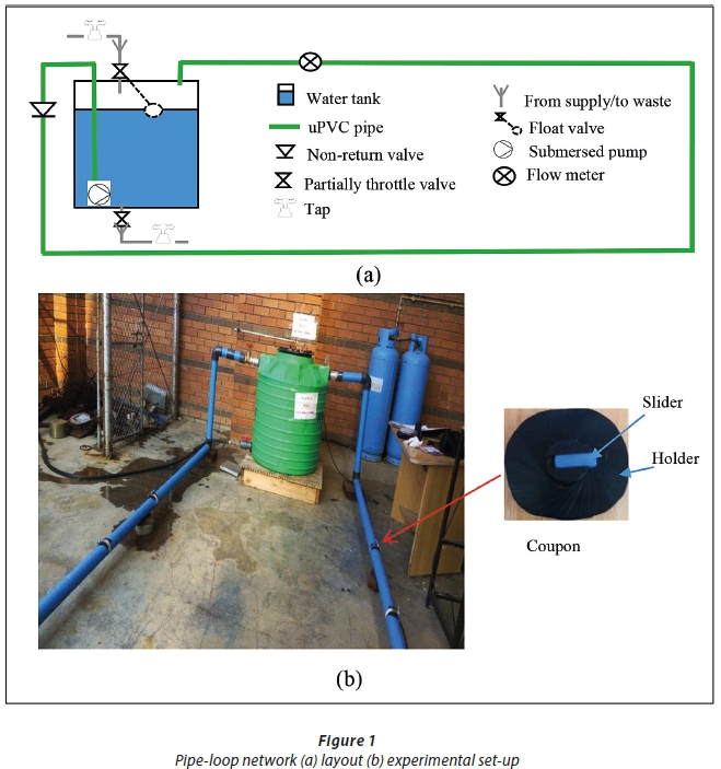
A new pipe-loop network was constructed to allow biofilm growth for a period of 5 months under conditions (constant flow rate, ambient temperature and pH of water) similar to the real distribution network, before the chlorine reaction rate constants were estimated. The pipe-loop network model (Fig. 1) was constructed using uPVC pipes of diameter 75 mm and length of 35 m connected to a 500 L tank. This type of pipe (uPVC) was selected because it constitutes more than 70% of the pipes in the GCWDS.
In order to provide favourable conditions for biofilm growth, water from the GCWDS was recirculated from the tank through the pipe-loop network using a submersed pump. The tank was emptied and refilled after every 48 h, directly from the distribution network of GCWDS. The flow rate in the pipe-loop network was kept at a constant rate of 0.4 L/s (velocity = 0.09 m/s), which is a typical flow rate in the main pipeline in the GCWDS.
Forty biofilm sampling devices (coupons) modified from Pennine water group coupon (Deines et al., 2010) were installed along the pipeline. Each coupon (Fig. 1) has a holder (diameter = 20 mm) fitted with a removable slider (width = 5 mm, length = 20 mm). The holders were made from rubber and the sliders were cut from the uPVC pipe used in the pilot network. The holders with sliders were fitted into the pipe wall using gaskets and pipe clamps. The pipe-loop network was cleaned before the start of the experiment by flushing with highly chlorinated water (10 mg/L) for 12 h. Each time the water tank was refilled, pH and temperature in the pipe-network model were recorded.
Two coupons were removed from the pipe-loop network model after every 7 days and accumulated biofilm cells quantified by the membrane filter method. First, a solution of the biofilm cells was prepared by the processes of harvesting, dispersion and dilutions. In the process of harvesting, 9 mL of distilled water was dispensed into a sterile tube (i.e. sample tube). The biofilms on the surface of the slider were scraped several times with a sterile applicator stick and then transferred into the sample tube. The stick was swirled vigorously in the sample tube to remove the biofilms. Using a sterile pipette, the scraped area of the slider was rinsed with 1.0 mL distilled water to remove the remaining biofilms and the solution also added into the sample tube. In the process of dispersion, the sample tube was put in a sonic water bath moving at a speed of 50-60 Hz for at least 2 min to separate the biofilm cells. A serial dilution solution of 10−1 (0.1 mL), 10−2 (0.01 mL) and 10−3 (0.001 mL) was prepared using the biofilm cell suspension in the sample tube. In the dilution process, 9 mL distilled water was dispensed into 3 dilution tubes. The sample tube was put on the vortex mixer for at least 8 s and 1.0 mL of the biofilm cell suspension was transferred from the sample tube to the first dilution tube (10−1). The first dilution tube was also put on the vortex mixer for about 8 s and 1.0 mL of the biofilm cell suspension was transferred to the second dilution tube (10−2). The preceding process was repeated to obtain the third dilution (10−3). The third dilution was then analysed by heterotrophic plate count using Standard Method for Examination of Water and Wastewater (SMEWW) 9215 D, the membrane filter method (APHA, 2005).
In order to estimate the chlorine reaction rate constants, chlorinated water from the GCWDS was circulated in the pipe-loop network for over 5 months to enable biofilm growth and obtain pipe wall conditions similar to a real WDS. After 5 months, 4 sets of pipe-loop network and bottle tests for chlorine concentrations were then performed simultaneously for 4 weeks with 1 set of tests per week. Table 1 presents the initial chlorine concentrations and flow conditions (all turbulent from the Reynolds number) that were used to perform each set of the pipe-loop network and bottle tests for chlorine concentrations. In each of the pipe-loop network tests, calcium hypochlorite was added into the water in the tank and mixed thoroughly to achieve the initial chlorine concentration. The chlorinated water was held in the tank for 1 h to allow calcium hypochlorite to fully dissolve and attain a homogeneous chlorine concentration before it was circulated in the pipe-loop network model. Chlorine concentrations in the water flowing in the pipe-loop network model were then measured after certain time intervals.

In bottle tests, 500 mL amber glass bottles were filled with the chlorinated water from the tank and kept in an incubator (20°C). One bottle was removed at a time from the incubator and tested for chlorine concentration at the same time that chlorine concentration was measured in the pipe-loop network. One-week intervals were allowed between the sets of the pipe-loop network and bottle tests to allow further growth of biofilm to ensure similar pipe and storage wall conditions for all of the experiments.
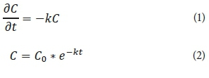
From the reaction rate (Eqs 1 and 2), assuming the reaction is first order, exponential plots of chlorine residual concentration (C) against time (t) for the pipe-loop network and bottle tests give the total reaction rate constant and bulk decay rate constant, respectively. The pipe wall reaction rate constant is computed as the difference between the total reaction rate constant and the bulk reaction rate constant (Zhou et al., 2004):
The pipe-loop network tests were carried out under ambient temperatures whereas bottle tests were carried out at 20°C. To compare their results, the van't Hoff-Arrhenius, Eq. 3, was used to adjust the estimated total reaction rate constants and bulk decay rate constants to the same temperature (T1 = ٢٠°C). In Eq. 3, θ is a conversion factor equal to 1.1 (Rossman, 2000), k1 and k2 are chlorine decay constants at temperatures T1 and T2 (ambient temperature in the pipe-loop network tests), respectively.

Analysis of the key water quality parameters in the study water distribution systems
Preliminary analysis of the following key water quality parameters in the water samples collected from selected locations in the GCWDS was conducted: chlorine residual, trihalomethanes (THMs), inorganic compounds (iron and manganese), natural organic matter (NOM), temperature and heterotrophic plate count (HPC). Total organic carbon (TOC), dissolved organic carbon (DOC) and ultraviolet absorbance at wavelength 254 nm (UVA-254) were used as surrogates for the NOM. Chlorine residual concentrations were tested immediately from the sampling sites using a multi-parameter hand-held colorimeter by DPD (N, N-Diethyl-p-phenylenediamine) indicator. Trihalomethanes (THMs) were analysed by liquid-liquid extraction and gas chromatography using EPA Method 551.1 (USEPA, 1990). Inorganic compounds (iron and manganese) were analysed by flame atomic absorption spectrometer (FAAS) using Standard Method for Examination of Water and Wastewater (SMEWW) 7000B (APHA, 2005). The TOC and DOC were analysed by TOC analysers and UVA-254 was analysed by ultraviolet (UV) spectrophotometer using EPA standard method 415.3 (USEPA, 2005). Heterotrophic plate count (HPC) in the water samples was performed using SMEWW 9215D membrane filtration method (APHA, 2005).
The water samples were collected from locations in the Phakalane distribution zone (PDZ) and Gaborone west distribution zone (GWDZ) as shown in Fig. 2. The sampling points selected at PDZ include; Mmamashia treatment plant (MTP) raw water (i.e. MTP-RW), Mmamashia treatment plant (MTP) treated water (i.e. MTP-TW), Oodi reservoir (OR), Phakalane reservoir (PR), Phakalane industrial tap (PIT) and Phakalane police tap (PPT). Note that PIT is located in a new network expansion area which is not yet mapped. The sampling points selected at GWDZ include: Gaborone treatment plant (GTP) raw water (i.e. GTP-RW), Gaborone treatment plant (GTP) treated water (i.e. GTP-TW), Forest Hill Reservoir (FHR), Bophirima Primary School tap (BPT) and Khuduga Primary School tap (KPT).

The samples for analysis of TOC, DOC and THMs were collected in 400 mL glass bottles preserved by adding sodium thiosulphate. The samples for analysis of inorganic compounds (iron and manganese) were collected in 400 mL high density polyethylene plastic bottles and preserved by adding nitric acid. All the samples were collected between 8:00 and 12:30 and transported in a portable ice-chest packed with ice and then stored at 4°C for analyses within 14 days. Samples for analysis of inorganic compounds and HPC were collected 6 times from each location between February 2016 and March 2016 at intervals of 1 week. These samples were analysed in the laboratory at the University of Botswana. However, samples for analysis of THMs and organic compounds (i.e. TOC and DOC) were collected 2 times at only the BPT sampling location in the GWDZ at 3-week intervals. These samples were analysed at the CSIR Laboratory at Stellenbosch, South Africa.
In this study, the water quality data were analysed by simple descriptive statistics using line and column charts. The line charts were used to show patterns in biofilm growth, temperature, and chlorine consumption rate in the pipe-loop network. The column charts of average (mean) values showing standard error bars were used to compare the occurrences of the following key water quality parameters at the selected locations in the GCWDS: chlorine residual, UVA-254, iron, manganese and HPC. The standard errors of the mean (SEM) were computed using Eq. 4 and indicate the spread of the data around the mean value and reliability of the mean value as a representative number for the dataset (Lee et al., 2015).

where s = standard deviation and n = number of data points in the sample.
RESULTS AND DISCUSSION
Biofilm growth and chlorine reaction rate constants
Figure 3 shows HPC (biofilm cell count) and water temperatures observed in the pipe-loop network over 5 months (February-June 2017). The results in Fig. 3 (a) indicate that biofilm cell count increased rapidly to over 800 CFU/100 mL in the first 2 months (February and March) but gradually decreased to below 300 CFU/100 mL in the last 3 months (April-June) of the experiment.

The decrease in biofilm cell count is partly attributed to low water temperatures in the month of April-June, shown in Fig. 3 (b). The results suggest higher biofilm growth rate in uPVC pipes in the GCWDS at high temperatures (> 20°C) during summer than the low temperatures in winter. This observation is in agreement with what was reported by LeChevallier (2003), where the occurrences of coliform bacteria and HPC were higher at temperatures above 15°C and peaked at temperatures of about 20°C in a pilot network. Biofilms act like reservoirs for microorganisms and contribute directly to bulk chlorine decay in WDSs (Bridier et al., 2011; Hallam et al., 2002; Wingenderand Flemming, 2011).
Figure 4 shows an example of an exponential plot of chlorine concentration against time for a bottle test and corresponding pipe-loop network tests used to estimate the total reaction, bulk decay and pipe wall decay rate constants that are presented in Table 2. Figure 5 shows the relative contribution of the bulk and pipe wall reactions to chlorine decay in the pipe-loop network.


It can be observed from Fig. 4 that the rate of chlorine decay was faster in the pipe-loop network than in the bottle test experiment. For instance, the amount of chlorine residual that remained after 10 h in the pipe-loop network was about 0.22 mg/L, which was lower than the bottle test value of about 0.68 mg/L. This is because the pipe-loop network results represent the total decay rate and the bottle test results present only residual chlorine reactions in the bulk of water in the network.
It is also evident from Fig. 5 that pipe wall decay rate constants were higher than bulk decay rate constants. The pipe wall decay rate constants were more than 50% of the total reaction rate constants, which indicates that pipe wall reaction contributed more to the chlorine decay in the pipe-loop network than bulk reaction did. These results were obtained under turbulent flow in the pipe-loop network. Similar work had shown higher bulk reaction rates than pipe wall reaction rates under low/steady flow conditions, whereas under laminar to turbulent flow, pipe wall reaction contributed more to the chlorine decay than bulk reaction did (Jamwal and Kumar, 2016). The results suggest that pipe wall conditions, such as biofilm growth and pipe material, consume more chlorine than reactions in the bulk of water that arise due to water quality conditions (i.e. organic and inorganic compounds), in the study WDS.
Figure 6 shows plots of chlorine residual against time for pipe-loop experiments demonstrating the effects of two different flow velocities on chlorine decay in the pipe-loop network. The results in Fig. 6 indicate that the chlorine decay rate was faster at a higher than a lower flow velocity. For instance, the amount of chlorine residual that remained after 9 h at a lower flow velocity (0.099 m/s) was about 0.25 mg/L whereas at a higher flow velocity (0.378 m/s) chlorine residual was about 0.1 mg/L. These results agree with other studies that a higher flow velocity causes release and re-suspension of biofilms in a distribution network, which imparts turbidity to piped water and accelerates the rate of chlorine consumption (Wingender and Flemming, 2004). Also, it is evident that pipe wall decay constants were higher at a high flow velocity in the pipe-loop network as shown in Table 2. These results agree with that of the study carried out by Digiano and Zhang, (2005), which attributed increase in pipe wall decay constant at a high flow velocity to increase in mass transfer rate of chlorine residuals to the wall of the pipe in the WDSs.

Occurrence of key water quality parameters
The average (mean) values of the concentration of the key water quality parameters presented through column charts were used to suggest their probable effects on chlorine decay in the GCWDS. Figure 7 shows the column charts of average (mean) chlorine residuals at selected locations in the PDZ and GWDZ with standard error bars. The results indicate that chlorine residuals in the treated water leaving both Mmamashia and Gaborone treatment plants (MTP-TW and GTP-TW) into the distribution network were about 1.5 mg/L, which is above the maximum standard limit of 1.0 mg/L required in WDSs according to the Botswana water quality standards.

At the selected customer taps (i.e. PIT, PPT, BPT and KPT in Fig. 2), the average chlorine residuals were lower than the minimum standard limit of 0.3 mg/L. The difference between chlorine residuals leaving the injection points and those at the customer taps was high (over 80%), which suggests a high rate of chlorine decay in the study network. The high chlorine injection rates at the treatment plants are potential sources of DBP formation, whereas the low levels of chlorine residuals at the customer taps expose drinking water to potential risks of microbial growth if contamination occurred in the network.
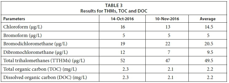
Table 3 shows the results for THMs, TOC and DOC in the water samples collected from the BPT (see location in Fig. 2) in the GWDZ. The results demonstrate that chloroform and bromodichloromethane had highest occurrences in the samples with average concentrations of 15 and 20.5 µg/L, respectively. The average total trihalomethanes (TTHMs) was 49.5 µg/L, which was below the regulated maximum allowable limit of 100 µg/L by the Botswana water quality standards. These low concentrations of THMs can be attributed to low levels of NOM measured by TOC and DOC concentrations (Table 3), in the treated water. However, strong correlations have been demonstrated in previous studies between THM formation and NOM, chlorine dosage and temperatures in the WDSs (Hassani et al., 2010; Samios et al., 2017; Toroz and Uyak, 2005). These preliminary analysis results have confirmed the occurrences of DBP formation in the GCWDS, which should inform further extended studies on DBP quantification, characterization and associated health risks. The results in Table 3 indicate that the average concentrations of TOC and DOC in the water samples were each 2.2 mg/L. Although this is below the maximum acceptable limit of 8 mg/L considered by the water quality standards in Botswana, it indicates the presence of TOC and DOC in the treated water.
Figure 8 shows the results of the UVA-254, which is used as a further surrogate to NOM in the water samples. The results indicate that the UVA-254 for both raw and treated water at the MTP was lower than that at the GTP. Also, there were significant levels of UVA-254 for the treated water (constituting more than a quarter (25%) of the average UVA-254 for raw water) at the treatment plants, reservoirs and the customer taps.

The presence of TOC, DOC and significant levels of UVA-254 in the water samples indicates that organic compounds contribute to chlorine decay in the GCWDS. Previous studies have shown a high correlation between chlorine bulk decay and NOM (i.e. TOC, DOC and UVA-254) in the WDSs (Al Heboos and Licsko, 2015; Hallam et al., 2003; Saidan et al., 2017).
Figure 9 shows the results for iron concentration in the water samples collected from the locations at PDZ and GWDZ. The results indicate that the average iron concentration in MTP-RW was quite low (0.249 mg/L) compared to GTP-RW (0.867 mg/L). The iron concentrations in treated water at all of the treatment plants, reservoirs and customer taps were lower than the regulated maximum limit of 0.3 mg/L. Therefore, it is unlikely that iron could have significantly contributed to chlorine decay, given its negligible concentrations in the WDS.

Figure 10 shows the results for manganese concentration in the water samples collected from the locations at PDZ and GWDZ. The results indicate that average manganese concentrations in both raw and treated water were below the regulated maximum limit (0.3 mg/L) and it is therefore unlikely that they could have contributed significantly to chlorine decay in the WDS.

Figure 11 shows the results for HPC, in CFU/100 mL, incubated at 35°C for ٤٨ h in m-HPC agar for the water samples collected from the locations at PDZ and GWDZ. The results indicate that there was a very high HPC (> 2 000 CFU/100 mL) in raw water and negligible HPC (< 100 CFU/100 mL) in the treated water at the treatment plants and reservoirs. However, the amount of HPC increased to between 100 and 300 CFU/100 mL at the customer taps, which indicates the existence of habitat such as biofilms and accumulated deposits that could provide favourable conditions for growth of microorganisms and chlorine decay in the GCWDS.

The recorded temperature of the water samples collected from the GCWDS (between 8:00 and 12:00 in March and April 2016) for the water quality analysis varied between 25 and 27°C. Figure 3 (b) shows the temperature of water in the pipe-loop network which was recorded at 21:00 during refilling of the tank. The temperatures in the pipe-loop network gradually dropped from about 26°C in February 2017 (summer) to about 11°C in June 2017 (winter). Previous studies have shown high correlation between chlorine decay and temperatures of water in the network (Hallam et al., 2003; Mutoti et al., 2007; Saidan et al., 2017). Therefore, temperature is also expected to be a contributing factor that leads to chlorine decay in the GCWDS. The pH recorded in both the WDS and pipe-loop network varied from 6.5 to 7.5 which is within the appropriate range (6-9) for effective chlorine disinfection.
CONCLUSIONS
This study investigated the probable causes of chlorine decay considering pipe wall conditions and distribution system water quality in the GCWDS. An experimental approach, which applies a pipe-loop network to estimate biofilm growth and chlorine reaction rate constants, was used to assess the pipe wall chlorine decay. Key water quality parameters that include chlorine residuals, TOC, DOC, inorganic compounds (iron, manganese), and HPC were analysed in water samples collected from selected locations in the GCWDS and their likely influences on chlorine decay assessed. The findings and conclusions made from the study are as follows:
•High biofilm cell count in the pipe-loop network (200-800 CFU/100 mL) and increase in HPC (100-300 CFU/100 mL) at the customer taps suggest that biofilm growth could have contributed significantly to chlorine decay in the study WDS. The results indicated increased biofilm growth rates at high temperatures (> 20°C) in summer relative to that at low temperatures in winter in the GCWDS.
•Pipe wall decay rate constants were higher than bulk decay rate constants in the pilot-loop network, which further suggests that pipe wall conditions such as biofilm growth and pipe materials increase the rate of chlorine decay more than reactions in the bulk of water that arise due to water quality conditions (i.e. organic and inorganic substances) in the study WDS.
•Presence of TOC and DOC (each 2.2 mg/L) and significant levels of UVA-254 for the treated water (i.e. UVA-254 of treated water constitutes about 25% of the UVA-254 for raw or untreated water) indicates that organic compounds had some contribution to chlorine decay and DBP formation in the GCWDS.
•Insignificant amounts of inorganic compounds (both iron and manganese < 0.3 mg/L) in the treated water indicate that they had minimal contribution to chlorine decay in the GCWDS.
•Based on information from this study, similar studies could be undertaken to investigate the causes of chlorine decay, in the other problematic areas of the GCWDS or any other WDS in the country or elsewhere. The inclusion of quantification and characterization of the major water quality parameters, such as natural organic matter and biofilms, that were found to be the probable causes of chlorine decay in the GCWDS in the current study, can be investigated in the future.
•Preliminary analysis in this study has also shown occurrences of disinfectant by-product (DBP) formation in the GCWDS, which should inform further extended studies on the DBP quantification, characterization and associated health risks.
ACKNOWLEDGEMENTS
We appreciate the support from the University of Botswana, Office of Research and Development (ORD), European Commission through Mobility to Enhance Training of Engineering Graduates in Africa (METEGA), Carnegie Cooperation through Regional Universities Forum for Capacity Building in Agriculture (RUFORUM), Gulu University and Water Utilities Corporation of Botswana.
CONFLICT OF INTEREST
There is no conflict of interest in this study.
REFERENCES
AL-JASSER AO (2007) Chlorine decay in drinking-water transmission and distribution ystems: Pipe service age effect. Water Res. 41 (2) 387-396. https://doi.org/10.1016/j.watres.2006.08.032 [ Links ]
AL HEBOOS S and LICSKO I (2015) Influence of water quality characters on kinetics of chlorine bulk decay in water distribution systems. Int. J. Appl. Sci. Technol. 5 (4) 64-73. [ Links ]
APHA (2005) Standard Methods for the Examination of Water and Waste Water (21st edn). American Public Health Association, Washington, DC. [ Links ]
BRIDIER A, BRIANDET R, THOMAS V and DUBOIS-BRISSONNET F (2011) Resistance of bacterial biofilms to disinfectants: a review. Biofouling 27 (9) 1017-1032. https://doi.org/10.1080/08927014.2011.626899 [ Links ]
CENTRAL STATISTICS OFFICE (2009) Botswana Water Statistics. URL: http://www1.eis.gov.bw/EIS/Reports/BotswanaWater_statistics report.pdf (Accessed 1 October 2017). [ Links ]
DEBORDE M and VON GUNTEN U (2008) Reactions of chlorine with inorganic and organic compounds during water treatment - Kinetics and mechanisms: A critical review. Water Res. 42 (1-2) 13-51. https://doi.org/10.1016/j.watres.2007.07.025 [ Links ]
DEINES P, SEKAR R, HUSBAND PS, BOXALL JB, OSBORN AM and BIGGS CA (2010) A new coupon design for simultaneous analysis of in situ microbial biofilm formation and community structure in drinking water distribution systems. Appl. Microbiol. Biotechnol. 87 (2) 749-756. https://doi.org/10.1007/s00253-010-2510-x [ Links ]
DEVARAKONDA V, MOUSSA NA, VANBLARICUM V, GINSBERG M and HOCK V (2010) Kinetics of free chlorine decay in water distribution networks. In: World Environmental and Water Resources Congress 2010: Challenges of Change. 4383-4392. https://doi.org/10.1061/41114(371)446 [ Links ]
DIGIANO FA and ZHANG W (2005) Pipe section reactor to evaluate chlorine-wall reaction. J. Am. Water Works Assoc. 97 (1) 74-85. https://doi.org/10.1002/j.1551-8833.2005.tb10805.x [ Links ]
GANG DC, CLEVENGER TE and BANERJI SK (2003) Modeling chlorine decay in surface water. J. Environ. Inf. 1 (1) 21-27. https://doi.org/10.3808/jei.200300003 [ Links ]
HALLAM NB, HUA F, WEST JR, FORSTER CF and SIMMS J (2003) Bulk decay of chlorine in water distribution systems. J. Water Resour. Plann. Manage. 129 (1) 78-81. https://doi.org/10.1061/(ASCE)0733-9496(2003)129:1(78) [ Links ]
HALLAM NB, WEST JR, FORSTER CF, POWELL JC and SPENCER I (2002) The decay of chlorine associated with the pipe wall in water distribution systems. Water Res. 36 (14) 3479-3488. https://doi.org/10.1016/S0043-1354(02)00056-8 [ Links ]
HASSANI AH, JAFARI MA and TORABIFAR B (2010) Trihalomethanes concentration in different components of water treatment plant and water distribution system in the north of Iran. Int. J. Environ. Res. 4 (4) 887-892. [ Links ]
HINCKLEY AF, BACHAND AM and REIF JS (2005) Late pregnancy exposures to disinfection by-products and growth-related birth outcomes. Environ. Health Perspect. 113 (12) 1808-1813. https://doi.org/10.1289/ehp.8282 [ Links ]
JAFVERT CT and VALENTINE RL (1992) Reaction scheme for the chlorination of ammoniacal water. Environ. Sci. Technol. 26 (3) 577-586. https://doi.org/10.1021/es00027a022 [ Links ]
JAMWAL P and KUMAR MSM (2016) Effect of flow velocity on chlorine decay in water distribution network: a pilot loop study. Current Sci. 111 (8) 1349. https://doi.org/10.18520/cs/v111/i8/1349-1354 [ Links ]
KARADIREK IE, KARA S, MUHAMMETOGLU A, MUHAMMETOGLU H and SOYUPAK S (2016) Management of chlorine dosing rates in urban water distribution networks using online continuous monitoring and modeling. Urban Water J. 13 (4) 345-359. https://doi.org/10.1080/1573062X.2014.992916 [ Links ]
KIENE L, LU W and LEVI Y (1998) Relative importance of the phenomena responsible for chlorine decay in drinking water distribution systems. Water Sci. Technol. 38 (6) 219-227. https://doi.org/10.2166/wst.1998.0255 [ Links ]
LECHEVALLIER MW (1999) Biofilms in drinking water distribution systems: Significance and control. Chapter 10 in: National Research Council (eds). Identifying Future Drinking Water Contaminants. The National Academies Press, Washington, DC. 206-260. https://doi.org/10.17226/9595.206-219. [ Links ]
LECHEVALLIER MW (2003) Conditions favouring coliform and HPC bacterial growth in drinking-water and on water contact surfaces. Heterotrophic Plate Count Measurement in Drinking Water Safety Management. Geneva, World Health Organization, 177-198. [ Links ]
MONTEIRO L, FIGUEIREDO D, COVAS D and MENAIA J (2017) Integrating water temperature in chlorine decay modelling: a case study. Urban Water J. 14 (10) 1097-1101. https://doi.org/10.1080/1573062X.2017.1363249 [ Links ]
MUTOTI G, DIETZ JD, AREVALO J and TAYLOR JS (2007) Combined chlorine dissipation: Pipe material, water quality, and hydraulic effects. J. Am. Water Works Assoc. 96-106. https://doi.org/10.1002/j.1551-8833.2007.tb08060.x [ Links ]
LEE DK, IN J and LEE S (2015) Standard deviation and standard error of the mean. Korean J. Anesthesiol. 68 (3) 220-223. https://doi.org/10.4097/kjae.2015.68.3.220 [ Links ]
PAVLOV D, DE-WET CME, GRABOW WOK and EHLERS MM (2004) Potentially pathogenic features of heterotrophic plate count bacteria isolated from treated and untreated drinking water. Int. J. Food Microbiol. 92 (3) 275-287. https://doi.org/10.1016/j.ijfoodmicro.2003.08.018 [ Links ]
PAYMENT P, FRANCO E, RICHARDSON L and SIEMIATYCKI J (1991) Gastrointestinal health effects associated with the consumption of drinking water produced by point-of-use domestic reverse-osmosis filtration units. Appl. Environ. Microbiol. 57 (4) 945-948. [ Links ]
POWELL JC, HALLAM NB, WEST JR, FORSTER CF and SIMMS J (2000) Factors which control bulk chlorine decay rates. Water Res. 34 (1) 117-126. https://doi.org/10.1016/S0043-1354(99)00097-4 [ Links ]
ROSSMAN LA (2000) EPANET 2 Users Manual. US Environmental Protection Agency. Water Supply and Water Resources Division, National Risk Management Research Laboratory, Cincinnati, OH, 45268. [ Links ]
ROSSMAN LA, CLARK RM and GRAYMAN WM (1994) Modeling chlorine residuals in drinking-water distribution systems. J. Environ. Eng. 120 (4) 803-820. https://doi.org/10.1061/(ASCE)0733-9372(1994)120:4(803) [ Links ]
SAIDAN MN, RAWAJFEH K, NASRALLAH S, MERIC S and MASHAL A (2017) Evaluation of factors affecting bulk chlorine decay kinetics for the Zai water supply system in Jordan. Case study. Environ. Protect. Eng. 43 (4) 223-231. [ Links ]
SAMIOS SA, GOLFINOPOULOS SK, ANDRZEJEWSKI P and ŚWIETLIK J (2017) Natural organic matter characterization by HPSEC and its contribution to trihalomethane formation in Athens water supply network. J. Environ. Sci. Health A Toxic/Hazardous Substances Environ. Eng. 52 (10) 979-985. https://doi.org/10.1080/10934529.2017.1324710 [ Links ]
STATISTICS BOTSWANA (2016) Botswana Environmental Statistics: Natural Disasters Digest 2015. Gaborone, Botswana. [ Links ]
TOROZ I and UYAK V (2005) Seasonal variations of trihalomethanes (THMs) in water distribution networks of Istanbul City. Desalination 176 (1) 127-141. https://doi.org/10.1016/j.desal.2004.11.008 [ Links ]
USEPA (1990) Determination of chlorinated disinfectant by products, chlorinated solvents and halogenatd pesticides/herbicides in drinking water by liquid-liquid extraction and gas chromatography with electron capture detection. Method 551.1. United States Environmental Protection Agency, Cincinnati, Ohio. [ Links ]
USEPA (2005) Determination of total organic carbon and specific UV absorbance at 254 nm in source water and drinking water. Method 415.3. United States Environmental Protection Agency, Cincinnati, Ohio. [ Links ]
VILLANUEVA CM, CANTOR KP, CORDIER S, JAAKKOLA JJK, KING WD, LYNCH CF, PORRU S and KOGEVINAS M (2004) Disinfection byproducts and bladder cancer: a pooled analysis. Epidemiology 15 (3) 357-367. [ Links ] VILLANUEVA CM, CANTOR KP, GRIMALT JO, MALATS N, SILVERMAN D, TARDON A, GARCIA-CLOSAS R, SERRA C, CARRATO A and CASTANO-VINYALS G (2007). Bladder cancer and exposure to water disinfection by-products through ingestion, bathing, showering, and swimming in pools. Am. J. Epidemiol. 165 (2) 148-156. https://doi.org/10.1093/aje/kwj364 [ Links ]
WINGENDER J and FLEMMING HC (2004) Contamination potential of drinking water distribution network biofilms. Water Sci. Technol. 49 (11-12) 277-286. https://doi.org/10.2166/wst.2004.0861 [ Links ]
WINGENDER J and FLEMMING HC (2011) Biofilms in drinking water and their role as reservoir for pathogens. Int. J. Hyg. Environ. Health 214 (6) 417-423. https://doi.org/10.1016/j.ijheh.2011.05.009 [ Links ]
WRIGHT JM, SCHWARTZ J and DOCKERY DW (2003) Effect of trihalomethane exposure on fetal development. Occup. Environ. Med. 60 (3) 173-180. https://doi.org/10.1136/oem.60.3.173 [ Links ]
WRIGHT JM, SCHWARTZ J and DOCKERY DW (2004) The effect of disinfection by-products and mutagenic activity on birth weight and gestational duration. Environ. Health Perspect. 112 (8) 920. https://doi.org/10.1289/ehp.6779 [ Links ]
ZHOU J, XUE G, ZHAO H, WANG YH and GUO MF (2004) Kinetics of chlorine decay in water distribution systems. J. Donghua University 21 (1) 140-145. [ Links ]
Received 13 July 2018
Accepted in revised form 6 March 2019
* To whom all correspondence should be addressed. e-mail: d.nono@gu.ac.ug

