ORIGINAL ARTICLES

 

Optimising intra-seasonal irrigation water allocation: Comparison between mixed integer nonlinear programming and differential evolution

 

 

B Grové^{I, *}; MC Du Plessis^II

^IDepartment of Agricultural Economics, University of the Free State, Bloemfontein, PO Box 339, Bloemfontein 9300, South Africa
^IIDepartment of Computing Sciences, Nelson Mandela University, Port Elizabeth, South Africa

 

 

---

ABSTRACT

Optimising crop planning in conjunction with intra-seasonal water allocation necessitates the use of daily water budget calculations to determine the timing and amount of irrigation events, which complicates the solution of the problem to global optimality. The main objective of this research was to compare the intra-seasonal water allocation of a mixed integer nonlinear programming (MINLP) model with that of differential evolution (DE), to allocate a limited amount of water while considering irrigable area and the irrigation schedule that will maximise the total gross margin. Results show that both solution procedures adhere to economic theory of water allocation under limited water supply. The conclusion is that the MINLP model most likely achieved very near global optimality as the solutions of the two models were very close to each other. DE holds promise to solve more complex models involving risk and multiple crops.

Keywords: intra-seasonal, water allocation, mixed integer nonlinear programming, differential evolution

---

 

 

INTRODUCTION

Dealing with increasing water scarcity will be an important research topic during the next decade, in the midst of producing enough food for a growing population (Paly et al., 2010). According to Garg and Dadhich (2014), there is a shift in research from maximising crop yield per unit area to increasing productivity of water through deficit irrigation under limited water supply conditions. English et al. (2002) also predicted a paradigm shift towards using economic principles to optimise agricultural water use in contrast to maximising crop yield. Providing decision support to irrigators for improved irrigation management under limited water supply conditions is extremely difficult, because irrigation management is a dynamic problem.

Crops grow through a process where water, abstracted from the soil water store, is transpired. Transpiration is reduced when the root zone soil water content drops below a crop specific threshold (Allen et al., 1998) and, consequently, the water deficit reduces crop yield. The onset of water deficit will only be known if the soil water content is tracked on a daily basis and the impact thereof on crop yield is determined by the sensitivity of a specific growth stage to the water deficit (Doorenbos and Kassam, 1979). Intra-seasonal water allocation is further complicated, because water availability on a per hectare basis is determined by the cropping area and available water. Thus, the irrigation scheduling decision (amount and timing) and the decision to plant a specific area must be considered simultaneously. Even if the allocation per hectare is known, the irrigator still needs to schedule water allocation to minimise electricity costs.

Intra-seasonal water allocation is not widely studied in South Africa. Botes et al. (1996) provide the most comprehensive treatment on the dynamics of intra-seasonal water allocation. The authors used a crop growth simulation model to determine the dynamic relationship between the soil water status and maize growth. Water use was optimised through linking the Nelder-Mead simplex algorithm to the crop growth simulation model. Botes et al. (1996) acknowledge that the intra-seasonal water allocation problem is characterised by many near-optimal solutions and did not consider the area irrigated as a decision variable. Schütze et al. (2012) argue that the solution procedure may fail when local optima exist or the number of decision variables become too large. Grové and Oosthuizen (2010) included area irrigated as a decision variable in their nonlinear programming model. However, these researchers approximated the dynamic interactions between soil water status and crop yield through the inclusion of 1 296 alternative irrigation schedules in their model. Achieving global optimality with such an approach is difficult when using time-of-use electricity tariff structures such as Ruraflex (Eskom, 2015/2016). In such a case, the irrigation schedules need to be optimised for the timing of water stress in conjunction with the time-of-use timeslots, which corresponds with lower electricity tariffs. As a result, the alternatives used to represent the problem might not include the best global solution. Recently, Venter and Grové (2016) developed a nonlinear programming model that incorporates daily water budget calculations to schedule irrigation events while considering detailed electricity cost calculations. The model includes area irrigated as a decision variable and could easily be applied to study the interaction between water availability, area irrigated and the timing and quantity of irrigation events. The square root approximations for the minimum and maximum functions used to model the water budget calculations, correctly make the constraint set highly non-linear and difficult to solve. One of the major problems of solving nonlinear programming models is that the solvers do not guarantee global optimality (Murtagh et al., 1998). Thus, the feasibility of the model solutions could only be judged on logical rationality.

An evolutionary algorithm (EA) provides an alternative means of solving complex intra-seasonal water allocation models (Shütze et al. 2012). The phrase EA refers to a class of stochastic optimisation algorithms inspired by biological evolution. The goal of these optimisation algorithms is to locate the global optima within a multidimensional search space in which local optima may be present. The global optimum is the best possible solution in the search space. A local optimum is a solution that is better than all surrounding solutions, but not as good as the global best solution.

An advantage of EAs is that they are relatively easy to implement, with the most complex part being the method to evaluate the quality of a given solution. Thus, the researcher does not have to specify how the problem should be solved, but only provides a means of determining how well a particular solution performs. A further advantage is that EA is suited to search spaces that are not differentiable, constrained or discontinuous, i.e., where the more traditional gradient-descent based algorithms cannot be used. Although the objective of an EA is to find the global optimum, there is no guarantee that it will be able to achieve this for any given problem. The algorithm could potentially be trapped in a local optimum, which constitutes an inferior solution. Various EAs exist in literature, including genetic algorithms (Holland, 1975), genetic programming (Koza, 1992), evolutionary programming (Fogel, 1962) and differential evolution (DE) (Storn, 1996). Differential evolution (Price, et al., 2005; Storn and Price, 1996; Storn and Price, 1997) is a relatively new addition to the EA family. Differential evolution has garnered considerable interest, because of its simplicity, effectiveness and general insensitivity to parameter settings. The application of DE within irrigation agriculture in South Africa is not new. Adeyemo and Otieno (2010) applied multi-objective DE to allocate areas irrigated between multiple crops based on full irrigation in the Vaalharts irrigation scheme. Apart from the multi-objectivity of their problem, the decision-making problem represented in this paper is much more complex as it represents the dynamic linkage between choosing the size of an irrigation area and scheduling irrigation water throughout the season dynamically on a daily basis.

The main objective of this research is to compare the intra-seasonal water allocation of a mixed integer nonlinear programming (MINLP) model with that of DE to allocate a limited amount of water while considering area irrigated and the irrigation schedule, which will maximise the total gross margin. Comparison of the results will allow a more formal judgement on the optimality of the MINLP model, and determine the suitability of using DE for optimising agricultural water use.

 

IRRIGATION ECONOMIC MODEL

The main purpose of the irrigation component of the irrigation economic model is to determine the impact of the timing and quantity of irrigation events on crop yield. Crop yield is linearly related to actual evapotranspiration (ETa) (Doorenbos and Kassam, 1979) and a key component of the irrigation model is to determine ETa. The level of ETa is a function of the root water content (RWC), because the level of evapotranspiration is reduced when the RWC falls below a threshold root water content (TRWC) (Allan et al., 1998). Consequently, daily water budget calculations are necessary to determine ETa. More specifically ETa is calculated on a daily basis as follows:

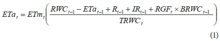
The numerator of the term in parenthesis represents the daily water budget calculations necessary to calculate RWC. The RWC as a fraction of the TRWC acts as a scaling factor with which potential evapotranspiration (ETm) is scaled to calculate ETa. The RWC is a function of the initial RWC, ETa, rainfall (R), net irrigation (IR) and any increases in the RWC due to root growth, which is a function of the water content below the root zone (BRWC) and the fraction of roots that grow into the zone (RGF). The RWC is limited not to exceed the amount of water that could be stored in the root zone and it is assumed that all excess water drains below the root zone. ETa is limited not to exceed ETm when the RWC is above the TRWC. Additions to the RWC due to root growth require knowledge of the BRWC, which requires a separate water budget calculation for the zone. The BRWC is calculated on a daily basis as follows:

The BRWC is a function of the initial BRWC, water that drains below the roots (BR) and the reduction in water content due to root growth where RGF represents the fraction of BRWC that will form part of RWC due to root growth. The BRWC is limited not to exceed the amount of water that could be stored in the zone below the roots and all excess water is assumed to drain below the zone.

Important to note is that IR represents the net amount of irrigation water that enters the soil. Thus, the amount does not take into account any inefficiencies. Inefficiencies may result from non-uniform water applications and wind drift. A constant wind drift loss of 10% (Van der Ryst, 1995) was assumed. Multiple water budgets (Hamilton et al., 1999) were modelled to incorporate inefficiencies that may have arisen due to non-uniform water applications. A distribution uniformity of 85% was assumed to determine the distribution of irrigation water across the water budgets. Only 3 water budgets were considered to keep the irrigation economic model tractable.

The relative evapotranspiration formula from Stewart et al. (1977) was used to relate relative evapotranspiration deficits to relative crop yield:

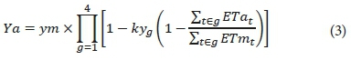
The formula distinguishes between 4 growth stages (g) that are characterised by different yield responses (ky) to evapotranspiration deficits. The multiplicative form allows the proportional decrease in potential crop yield (Ym) to be more if the crop is stressed in more than one crop growth stage. The crop yield and daily irrigation output from the irrigation component was used in the economics component to calculate the resulting total gross margin as follows:

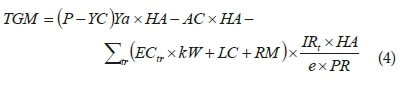
The first term, (P−YC)Ya x HA calculates gross income minus yield-dependent costs (YC) while the second term, AC x HA, accounts for the total area dependent costs (AC) for the area (HA) irrigated. The last term calculates the irrigationdependent costs, which include electricity costs (EC), labour costs (LC) and repair and maintenance costs (RM). Irrigation system-specific parameters in the calculation comprised kilowatt requirement (kW), pumping rate (PR) and irrigation system application efficiency (e). Of note is that EC is defined for a specific day (t) as well as the specific Ruraflex time-of-use time period during the day (r). As a result, the effect of irrigation during periods with high electricity tariffs was captured in the total gross margin calculation for the pivot.

 

DATA AND ANALYSES

Venter (2015) compiled a dataset with all the necessary weather, crop, soil, irrigation system-specific and cost parameters required to populate the irrigation economic model for maize grown at Douglas under centre pivot irrigation. Weather-dependent parameters include rainfall and maximum evapotranspiration rates derived from weather data. Crop parameters include Kc-values to relate maximum evapotranspiration rates to the evapotranspiration rates of maize, and Ky-values to relate crop water deficits to crop yield and root growth. Soil information relates to the soil water-holding capacity, which was assumed as 130 mm/m, and the threshold water content beyond which the crop will start to experience water stress. The size of the pivot was 30 ha and the irrigation system capacity was 10 mm/day. The uniformity of water applications was assumed to be 85%, which implied that a third of the area was under- irrigated by 30% and a third was over-irrigated by 30% (Li, 1988) when a uniform distribution between the maximum and minimum amounts was assumed. The costs in the dataset include enterprise budgets for maize as well as electricity costs for the 2013/14 production season. The database was not updated as the sole purpose of this paper is to compare the results obtained with the MINLP and DE models with the aim of scrutinizing the global optimality of the MINLP solver.

The irrigation economic model was solved for 8 different water allocations ranging from 75 mm/ha listed to 600 mm/ha listed. The total area listed is 30 ha. The range of water availabilities were chosen such that the results included both water-limiting and area-limiting phases of production.

Mixed integer nonlinear programming solver

Before solving the model with the MINLP solver, it is necessary to represent the model within a constrained optimisation framework. Representing the water budget calculations of the irrigation component within a constrained optimisation framework is troublesome, because boundary conditions need to be set for the variables that define the water budget calculations. Using minimum and maximum functions to impose the boundary conditions is not recommended, as these functions are discontinuous and therefore not differentiable (GAMS Development Corporation, 2017). The smooth approximation of the minimum and maximum functions proposed by the GAMS Development Corporation (2017) is used to ensure that the equations are differentiable. For a complete implementation of the model using the smooth approximation approach, the reader is referred to Venter (2015). Binary variables were introduced to ensure that the net irrigation amounted to zero or between 6 mm/day and 9 mm/day.

The irrigation economic model was constructed in GAMS (GAMS Development Corporation, 2017) and solved with GAMS/DICOPT, which required a nonlinear programming (NLP) solver and mixed integer programming (MIP) solver. GAMS/MINOS and GAMS/CPLEX were selected as the NLP and MIP solvers, respectively. The complete irrigation economics model consisted of 1 808 equations and 1 544 variables. At first the model was constructed such that an irrigation event could take place on any of the 120 growing days. However, the model failed to solve and the process was terminated. The model was then simplified by restricting irrigation events to every second day while leaving the possibility to irrigate between a minimum of 6 mm and a maximum of 18 mm, which corresponded to 2 days of water application. By implication, the model was allowed to spread the irrigation hours over a 2-day period even though enough hours might have been available to irrigate the designated amount of water on 1 day. Thus, the model was able to make better utilization of the off-peak hours. In the process, the dimension of the programming model was reduced to 1 388 equations and 1 244 variables.

Differential evolution

DE is a stochastic optimisation algorithm inspired by biological evolution that iteratively optimises a set (referred to as population) of potential solutions (referred to as individuals). Iterations are called generations, as components from individuals in the current population are combined to form the individuals of an offspring population. The population entering the next iteration is made up of better performing individuals than the previous populations. In general, the following pseudo-code describes the working of the DE algorithm for a maximisation problem:

Initialise a random population of individuals (candidate solutions)

While termination criteria are not met do

For each individual in the current population do

Randomly select 3 individuals from the population: and

Create a new vector as follows:

where F is a constant

Create a new vector as follows:

 

where j_r is a randomly selected vector index and C is a constant

For each individual in the current population do

If Fitness < Fitness() then replace with

The concept of fitness is central to the functioning of DE. The fitness is a measure of how well a particular individual solves the problem at hand. In the current application, the total gross margin generated was used to evaluate the fitness of the individuals.

Individuals (candidate solutions) in a DE population are viewed as vectors in the search space. The core idea behind DE is that the vector differences between individuals are used to perturb parent individuals when creating offspring. This provides a natural means of controlling the exploration of the population. Initially, when the population is widely distributed (this is referred to as having high diversity), the vector differences would be large, thus resulting in large perturbations and more exploration of the search space. Eventually, as the population converges to a solution, the vector differences would be small (low diversity), resulting in a fine-grained exploitative search around the optimum.

The algorithm thus has 3 parameters: the population size, F and C. These last two parameters are normally set within the range [0,1] and can be tuned to change the exploration and exploitation behaviour of the algorithm. Although guidelines for appropriate settings for F and C can be found in the literature (Storn, 1996; Pedersen, 2010; Rönkkönen et al., 2005), it is best to find problem-appropriate values for these parameters by testing a range of values during preliminary experiments.

Differential evolution implementation for the irrigation problem

The goal of the optimisation process is to determine the irrigated area in hectares and the irrigation schedule that should be followed to maximise total gross margin of maize production within the constraints of the problem. The constraints that were imposed included the maximum amount of water that can be irrigated in a single day (IR_Max), the minimum amount of water that can be given on a day when irrigation occurs (IR_Min), the total amount of water that can be applied during the entire season (IR_Total and the maximum number of hectares that can be planted (Ha_Max).

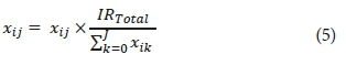
The nature of the DE is that the hectares irrigated and the irrigation schedule can be directly encoded as an individual. Each individual thus consists of an array of real values. One of these values represents the number of hectares that should be placed under irrigation. The remainder of the array values represent the amount of water that must be irrigated on each successive day of the production season. The population is initialised by creating random individuals. The array values for each individual are assigned a random real value between 0 and IR_Max for the irrigation values, and 0 and Ha_Max for the number of hectares to be planted. A hard constraint is implemented that ensures that the values always fall within the initialisation ranges during the entire evolution process. Invalid values are prevented by clipping each array value to the valid range as soon as the individuals are created. Values that exceed IR_Max are set to IR_Max. However, values below IR_Min are left unchanged, although these values are treated as zero when fitness calculations are performed. This approach is analogous to the concept of recessive genes in biology. Encoded information is passed from one generation to the next, although this information is not necessarily expressed by the individual. The constraint where the total amount of water used for irrigation during a season must not exceed IR_Total is more complex to incorporate into the algorithm. Individuals were physically corrected to ensure compliance with this constraint. This was achieved by scaling the irrigation value for each day in the season by the ratio by which the total budget was exceed. So, for each individual in the population for which > IR_Total where J is the total number of days in the production season) the irrigation amount for each day was adapted as follows:

This technique ensures that the water budget is not exceeded, without biasing the algorithm towards any particular watering scheme.

The DE algorithm as well as the irrigation economics model that is used to simulate the fitness of each individual were coded in the Java programming language. Preliminary experiments found that parameter values of F = 0.3 and C = 0.7 worked well. Due to the stochastic nature of the DE algorithm, each optimisation at a specified water allocation was done 30 times and the best one was retained as the optimal solution. Daily irrigation events were allowed, which was the only difference between the MINLP solver and the DE algorithm.

 

RESULTS

Objective / fitness function

The total gross margin, hectares irrigated and the resulting crop yield, optimised with the MINLP solver and the DE algorithm, are given in Table 1. The results show that the MINLP solver outperformed the DE algorithm in terms of achieving a higher total gross margin. Whether the MINLP solver achieved global optimal solutions is open to debate. Maize productivity plateaued at the maximum potential maize yield of 17 t/ha when water allocations exceeded 525 mm/ha for the 30 ha listed for both MINLP and DE. Thus, water allocation in excess of 525 mm is associated with abundant water supply and both the solvers are expected to reach maximum potential gross margins resulting from maximum potential maize yields on fully utilised irrigation areas. Interestingly, the total gross margin of a water allocation of 600 mm is lower than the 525 mm allocation when considering the MINLP solutions. Such a result is an indication that the MINLP solver fails to identify the maximum outcome if water is unlimited and multiple irrigation schedules characterise the optimal solution. The DE algorithm achieved the same results for unlimited water supply which is more logical; however, total gross margins were lower when compared to the MINLP solutions. The DE algorithm was able to achieve a slightly higher total gross margin for a water allocation of 450 mm. The optimised total gross margin results for the DE algorithm showed a close resemblance to that of the MINLP solver, even though most of the optimised values were lower than that of the MINLP solver solutions. The largest difference was 0.45%.

Two distinct phases were identifiable from the results, depending on whether water or land was the most limiting factor of production. During the water-limited phase (75 mm-300 mm), it was profitable to deficit-irrigate the crop and to use the saved water to irrigate a larger area. The total gross margins increased linearly during the water-limited phase, because the optimal level of deficit irrigation did not change as long as water was the limiting factor. Consequently, crop yield per hectare was the same and any increases in total gross margin were attributed to increases in irrigated area. The area-limited phase commenced from a water allocation of 375 mm. During the area-limited phase, water was not the most limiting factor of production and any additional water was used to increase crop yields per hectare. Declining marginal productivity characterised the area-limited phase and the total gross margins increased at a decreasing rate when more water was applied per hectare. Interestingly near maximum crop yield per hectare was achieved under water abundance, which indicated that electricity costs and water tariffs were still low compared to the value of the marginal product of applying an additional unit of water.

A key part of the irrigation scheduling problem is to schedule the timing and irrigation amounts to achieve good crop yields. The problem is further complicated when water is pumped during the Ruraflex timeslots with lower electricity tariffs, thereby reducing irrigation costs. Table 2 shows the optimised distribution of pumping hours during the different Ruraflex time-of-use timeslots for the MINLP solver and the DE algorithm.

The optimised distribution of pumping hours obtained with the MINLP solver for each water allocation showed that a larger proportion of the water was pumped during off-peak hours when compared with the distribution obtained with the DE algorithm. Thus, the total electricity cost of the MINLP solver was lower in all instances except for a water allocation of 75 mm where the cost was the same. A larger allocation of pumping hours to standard tariff timeslots was the direct result of not allowing the DE algorithm to allocate pumping hours over 2 days. Changing the DE algorithm to allocate pumping hours over 2 consecutive days may have resulted in the difference between the two solution procedures being reduced further.

The importance of keeping track of the soil water status was accentuated by the results, because it was optimal to irrigate in standard and even peak timeslots to ensure good crop yield per hectare. The large difference between the hour distribution of the MINLP solver and the DE algorithm while achieving similar total gross margins further showed that numerous solutions existed that were close to the optimal solution.

Irrigation schedules

Previously it was argued that the same level of deficit irrigation was optimal in the water-limited phase of production. By implication, the irrigation schedules in the water-limited phase should all be the same irrespective of water allocation, as long as water is the most limiting factor of production. Figure 1 and Figure 2, respectively, show the irrigation schedules optimised with the MINLP solver and the DE algorithm for the water-limited phase of production.

 

 

 

 

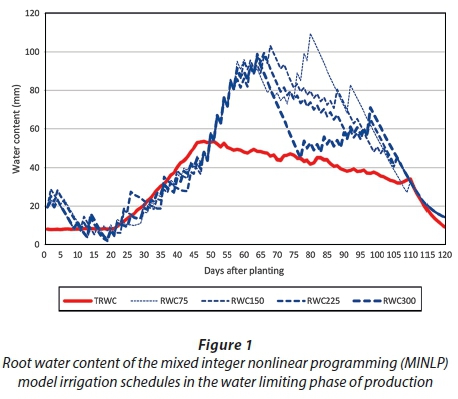
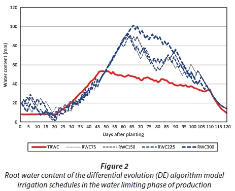
The irrigation schedules for both solution procedures demonstrated that a variety of irrigation schedules yielded similar results. The diversity of the MINLP solver irrigation schedules seemed higher when compared with the irrigation schedules of the DE algorithm. Such a result is surprising given the fact that the DE algorithm is a stochastic process. The irrigation schedules of both solution procedures did, however, exhibit some important characteristics. Water stress set in when the RWC of the irrigation schedule was below TRWC. The results from Figs ١ and ٢ clearly show that the RWC of both solution procedures fell below TRWC most of the time during establishment and vegetative crop growth stages (Days 1-49) when the crop was less sensitive to water deficits. Both solution procedures ensured that the RWCs of the irrigation schedules were above the TRWC between Days 50-110 when the crop was most sensitive to water deficits, while no irrigation water was applied during the last 10 days in both models.

 

DISCUSSION AND CONCLUSIONS

The main conclusion from this research is that the MINLP model specification of the intra-seasonal water allocation problem provided answers that were likely to be close to the global optima. This was because the MINLP model solutions were close to the DE solutions, which were determined with the more robust solution procedure. Despite both models independently finding almost identical solutions, global optimality could, however, not be guaranteed. It is common knowledge that it is more difficult to use nonlinear programming to solve a problem if the non-linearity is confined to the constraint set. It may be possible to reformulate the square root approximations into linear functions using disjunction (Nemhauser and Wolsey, 1999) to aid the discovery of the global optimal solution.

The ease with which the DE algorithm is applied to the intra-seasonal water allocation problem and the quality of the results is encouraging. Preliminary results of testing a stochastic representation of the intra-seasonal water allocation problem seem promising, especially if one considers that the mathematical programming model formulation of the same problem could not be solved with the same solvers used in this research. The robustness of the algorithm should further be tested.

 

ACKNOWLEDGEMENTS

The paper is based on research being conducted as part of a solicited research project, 'Long-run hydrolic and economic risk simulation and optimization of water curtailments' (K5/2498//4), that is initiated, managed and funded by the Water Research Commission (WRC, 2015). Financial and other assistance by the Water Research Commission is gratefully acknowledged.

 

REFERENCES

ADEYEMO J and OTIENO F (2010) Differential evolution algorithm for solving multi-objective crop planning model. Agric. Water Manage. 97 848-856. https://doi.org/10.1016/j.agwat.2010.01.013        [ Links ]

ALLEN RG, PEREIRA L, RAES D and SMITH M (1998) Crop evapotranspiration: Guidelines for computing crop water requirements. FAO Irrigation and Drainage Paper No 56. FAO, Rome.         [ Links ]

BOTES JHF, BOSCH DJ and OOSTHUIZEN LK (1996) A simulation and optimization approach for evaluating irrigation information. Agric. Syst. 51 165-183. https://doi.org/10.1016/0308-521X(95)00042-4        [ Links ]

DOORENBOS J and KASSAM AH (1979) Yield response to water. FAO Irrigation and Drainage Paper No 33. FAO, Rome.         [ Links ]

ENGLISH MJ, SOLOMON KH and HOFFMAN GJ (2002) A paradigm shift in irrigation management. J. Irrig. Drain. Eng. 128 (5) 267-277. https://doi.org/10.1061/(ASCE)0733-9437(2002)128:5(267)        [ Links ]

ESKOM (2015/16) Tariffs and charges booklet. URL: http://www.eskom.co.za/content/2015_16DraftTariffBookver3.pdf (Accessed 21 January 2016).         [ Links ]

FOGEL LJ (1962) Autonomous automata. Ind. Res. 4 14-19.         [ Links ]

GAMS DEVELOPMENT CORPORATION (2017) GAMS documentation, Distribution 24.9. Gams Development Corporation, Washington DC.         [ Links ]

GARG NK and DADHICH SM (2014) Integrated non-linear model of optimal pattern and irrigation scheduling under deficit irrigation. Agric. Water Manage. 140 1-13. https://doi.org/10.1016/j.agwat.2014.03.008        [ Links ]

GROVÉ B and OOSTHUIZEN LK (2010) Stochastic efficiency analysis of deficit irrigation with standard risk aversion. Agric. Water Manage. 97 (6) 792-800. https://doi.org/10.1016/j.agwat.2009.12.010        [ Links ]

HAMILTON JR, GREEN GP and HOLLAND D (1999) Modeling the reallocation of Snake river water for endangered salmon. Am. J. Agric. Econ. 81 (5) 1252-1256. https://doi.org/10.2307/1244117        [ Links ]

HOLLAND J (1975) Adaptation in Natural and Artificial Systems. University of Michigan Press, Michigan.         [ Links ]

KOZA JR (1992) On the Programming of Computers by Means of Natural Selection. MIT Press, Cambridge, Massachusetts.         [ Links ]

LI J (1998) Modeling crop yield as affected by uniformity of sprinkler irrigation system. Agric. Water Manage. 38 (2) 135-146. https://doi.org/10.1016/S0378-3774(98)00055-9        [ Links ]

NEMHAUSER GL and WOLSEY LA (1999) Integer and Combinatorial Optimization. Wiley, New York.         [ Links ]

PALY M, SCHÜTZE N and ZELL A (2010) Determining crop-production functions using multi-objective evolutionary algorithms. In: Proceedings of the 2010 Congress on Evolutionary Computation, 18-23 July 2010, Barcelona, Spain.         [ Links ]

PEDERSEN MEH (2010) Good parameters for differential evolution. Technical Report HL1002, Hvass Laboratories, Copenhagen, Denmark.         [ Links ]

PRICE K, STORN R and LAMPINEN J (2005) Differential Evolution - A Practical Approach to Global Optimization. Springer, Berlin.         [ Links ]

RÖNKKÖNEN J, KUKKONEN S and PRICE KV (2005) Real-parameter optimization with differential evolution. In: Proc. 2005 Congress on Evolutionary Computation, 2-5 September 2005, Edinburgh. https://doi.org/10.1109/CEC.2005.1554725        [ Links ]

SCHÜTZE N, PALY M and SHAMIR (2012) Novel simulation-based algorithms for optimal open-loop and closed-loop scheduling of deficit irrigation systems. J. Hydroinf. 14 (1) 136-151. https://doi.org/10.2166/hydro.2011.073        [ Links ]

STEWART, JI, HAGAN RM, PRUITT WO, DANIELSON RE, FRANKLIN WT, HANKS RJ, RILEY JP and JACKSON EB (1977) Optimizing crop production through control of water and salinity levels in the soil. Reports, Paper 67. URL: https://digitalcommons.usu.edu/water_rep/67        [ Links ]

STORN R (1996) On the usage of differential evolution for function optimization. In: Proc. 1996 Biennial Conference of the North American Fuzzy Information Processing Society, 19-22 June 1996, Berkeley, California, USA. https://doi.org/10.1109/NAFIPS.1996.534789        [ Links ]

STORN R and PRICE K (1996) Minimizing the real functions of the ICEC'96 contest by differential evolution. In: Proc. 1996 IEEE International Conference on Evolutionary Computation, 20-22 May 1996, Nagoya, Japan. https://doi.org/10.1109/ICEC.1996.542711        [ Links ]

STORN R and PRICE K (1997) Differential evolution - a simple and efficient heuristic for global optimization over continuous spaces. J. Glob. Optim. 11 (4) 341-359. https://doi.org/10.1023/A:1008202821328        [ Links ]

VAN DER RYST C (1995) Evaporati0on and wind drift losses during centre pivot irrigation. Proc. Southern African Irrigation Symposium, 4-6 June 1991, Durban. WRC Report No. 379/1/96. Water Research Commission, Pretoria.         [ Links ]

VENTER M (2015) Modelling the economic trade-offs of irrigation pipeline investments for improved energy management. MSc dissertation, University of the Free State.         [ Links ]

VENTER M and GROVÉ B (2016) Modelling the economic trade-offs of irrigation pipeline investments for improved energy management. Water SA 42 (4) 542-550. https://doi.org/10.4314/wsa.v42i4.04        [ Links ]

WRC (Water Research Commission) (2015) WRC Knowledge Review 2015/16. Water Research Commission, South Africa.         [ Links ]

 

 

Received 24 November 2017
Accepted in revised form 4 December 2018.

 

 

* To whom all correspondence should be addressed. e-mail: GroveB@ufs.ac.za