ORIGINAL ARTICLES

 

Mathematical modelling and analysis of the flocculation process in low retention time hydraulic flocculators

 

 

Danieli Soares de Oliveira^{I, *}; Clainer Bravin Donadel^II

^IIFES - Federal Institute of Espírito Santo, Rodovia Governador José Sette, 184 Itacibá, Cariacica ES, 29150410, Brazil
^IIIFES - Federal Institute of Espírito Santo, Avenida Vitória, 1729, Jucutuquara, Vitória ES, 29040780, Brazil

 

 

---

ABSTRACT

This article aims to advance the understanding of particle interactions in low retention time flocculators and proposes a new flocculation model that appropriately considers the influence of retention time in flocculation processes. This consideration is important for units with flocculation time lower than 1 min, as seen in helically coiled tube flocculators (HCTFs), whose retention time is significantly lower than conventional flocculation units (about 30 min). With this, it was possible to obtain a more adherent model, reducing deviations between results obtained by physical modelling (using HCTFs, 48 tests) and those obtained with the proposed model, when compared with results obtained using the flocculation models commonly used for this purpose. The decreasing-rising behaviour presented by experimental data for process efficiency versus retention time, not verified in the benchmark models, was satisfactorily addressed by the proposed model. Furthermore, maximum and average absolute percentage deviations obtained using the model proposed in this study were less than or equal to the results obtained with the benchmark models and less for experimental uncertainty (10%). The results obtained indicate that this model can be a useful tool to support the rational design of low retention time units, including applications for the water industry and water recycling systems.

Keywords: flocculation models, helically coiled tube flocculators (HCTFs), hydraulic flocculators, mathematical modelling, physical modelling

---

 

 

INTRODUCTION

Clarification is an important stage in the physical-chemical water and wastewater treatment process and has great theoretical and practical importance, including applications for the water industry and water recycling systems, using chemical and/or bioflocculants (Khannous et al., 2011; Ugbenyen and Okoh, 2014; Maceda-Veiga et al., 2015; Mudhiriza et al., 2015; Agunbiade et al., 2016; Ma et al., 2017; Shaikh et al., 2017; Watanabe, 2017). It is fully dependent on the interaction between suspended particles present in fluids, since this interaction promotes floc formation and breakup. Such interactions can primarily occur in three ways: perikinetic interaction, orthokinetic interaction and interaction by differential sedimentation.

In perikinetic interaction, also known as Brownian motion, the irregular motion of particles leads to a collision between them. This kind of interaction is relevant only when particles have a reduced size (about 1 µm; Bratby et al. (1977)). In orthokinetic interaction, an external source of energy is necessary to promote particle collisions, commonly with size higher than 1 µm. The added energy generates velocity gradients in the flow, both in laminar or turbulent flow. In interaction by differential sedimentation, discrete particles with different features (for instance: porosity, density, size and shape) have different sedimentation velocities, leading to collisions between particles moving with different velocities.

Among these interaction modes, only orthokinetic interactions are relevant in flocculation units commonly used in the water treatment process (Bratby et al., 1977), in which the agitation of liquid mass should be high enough to ensure the contact between particles and should be low enough to avoid the breakup of existing flocs.

In this context, mathematical models for orthokinetic interactions have been proposed in the literature (Smoluchowski, 1917; Camp and Stein, 1943; Fair and Gemmell, 1964; Hudson, 1965; Harris et al., 1966; Argaman, 1968; Argaman and Kaufman, 1970; Bratby et al., 1977; Libânio et al., 1996; Son and Hsu, 2008; Weber-Shirk and Lion, 2010; Moruzzi and Oliveira, 2012; Cottereau et al., 2014; Sithebe and Chirwa, 2016). Most of the presented models do not appropriately consider the influence of retention time in flocculation processes. This assumption is valid only for higher retention times, commonly verified in conventional flocculation units (with retention times of about 30 min). Therefore, this paper aims to propose a new flocculation model, adherent to flocculation units with low retention times (with retention times of about 1 min), and able to appropriately considers the influence of retention time in the flocculation process.

Literature review

The first study that presented a mathematical model for interactions in laminar flow was by Smoluchowski (1917). In his study, Smoluchowski (1917) presented an expression for flocculation rate in a particle size distribution bimodal system (Eq. 1). The Smoluchowski model can also be used in combination with different theories, like fractal theory (Yang et al., 2013).

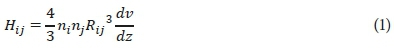
Similar to Smoluchowski (1917), Camp and Stein (1943) proposed a model that describes the contact between two particle with radius R_i and R_j, replacing the velocity gradient (dv/dz) by the root mean square value of unit's velocity gradient (G). The interaction between two particles with different sizes is presented in Fig. 1.

 

 

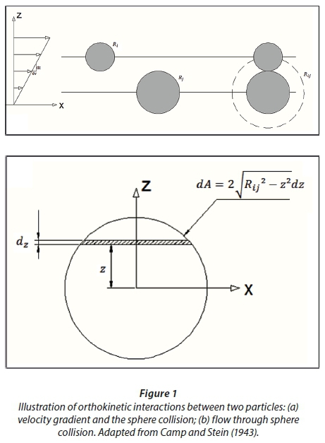
Contact between particles with radius R_i and R_j is possible if the volume delimited by the sphere collision (represented by a dashed circle in Fig. 1-a, with radius R_ij) was crossed. Therefore, contact between particles with radius R_i and R_j is possible if the center of the particle with radius R_i crosses the dashed circle in Fig. 1a.

The flow through the fluid sphere in Fig. 1 can be determined from the integration of the differential flow, dq, in a differential area with thickness dz in the entire sphere, as shown in Fig. 1b. Differential flow dq is given by Eq. 2:

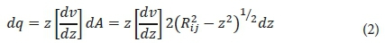
Integrating Eq. 2 along the sphere collision's surface, the flow rate in the sphere is obtained. Considering that (a) the number of collisions per unit of time (H_ij) between particles is given by the product of the flow rate in sphere collision (q) and the number of particles per unit of volume (n_i and n_j), and (b) the velocity gradient (dv/dz) term can be replaced by the root mean square value of the unit's velocity gradient (G), the orthokinetic interactions rate between discrete particles can be obtained - Eq. 3:

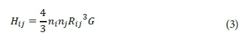
From Eq. 3, it is possible to verify the relation between the particle collision rate and the hydrodynamic parameter velocity gradient, beyond the relation between particle collision rate and particles' size existing in the fluid mass.

Another study that developed a flocculation mathematical model based on Eq. 1 presented in Smoluchowski (1917) is Fair and Gemmell (1964). These authors proposed a model to describe the variation of particle number (n_k) related to a specific size class (k) - Eq. 4.

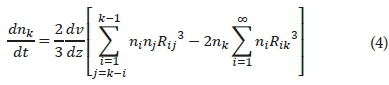
It is important to note that the models presented in Eqs 2, 3 and 4, do not consider the failure probability in the flocculation process (in case of failure flocs are not formed, even if collisions between particles occur). Furthermore, these models considered that all collisions lead to bigger flocs. There is no term to represent floc breakup.

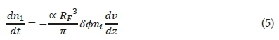
Terms related to floc breakup began to be included in the models of Harris et al. (1966), which modified Eq. 4, inserting a new term related to floc breakup. Failure probability in the flocculation process was considered through the insertion of parameter ∝, related to the fraction of collisions that result in flocs. The proposed model is presented in Eq. 5:

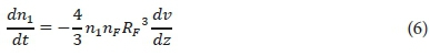
However, Hudson (1965) considered a bimodal distribution system for particle size, being such a system composed by discrete particles and flocs, and assuming that variations in elements' size within each group are small when compared with the difference between the size of elements of each group. In this system, discrete particles are removed from the liquid mass through their collision with flocs. Therefore, Eq. 4 is simplified, as shown in Eq. 6:

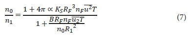
In order to include a parameter related to floc breakup and retaining the bimodal distribution system concept, Argaman (1968) and Argaman and Kaufman (1970) presented an orthokinetic flocculation model similar to the model presented by Smoluchowski (1917). This model is based on the hypothesis that discrete particles in a turbulent flow are in random movement like Brownian motion, inherent to perikinetic interaction. Another hypothesis assumed in this model is the utilization of a bimodal distribution system for particle size, similar to the system adopted in Hudson (1965). Argaman (1968) and Argaman and Kaufman (1970) confirmed the proposed system experimentally through the evaluation of floc size.

The model proposed by Argaman (1968) and Argaman and Kaufman (1970) considers two different processes to modify particle concentration: aggregation of discrete particles and floc breakup - Eq. 7:

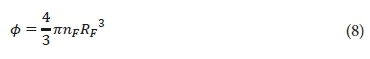
In order to make Eq. 7 viable for practical purposes and allow the parameter to be obtained experimentally, three considerations were performed: (i) the average size of flocs is directly related to mean square velocity fluctuations (R_F = K₂/(u²)_average); (ii) the mean square velocity fluctuations can be estimated from root mean square value of unit's velocity gradient ((u²)_average = K_P.G); and (c) particles and flocs are considered spheres - therefore, the fraction of floc volume is given by Eq. 8:

Grouping constants in two classes, the first one being related to particle aggregation (K_A) and the second related to floc breakup (K_B), the model expressing the function of K_A and K_B is given by Eq. 9:

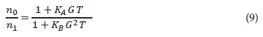
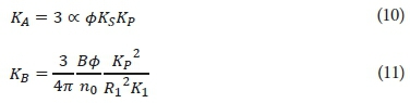
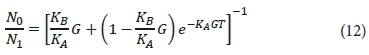
Where K_A and K_B are given by Eqs 10 and 11:

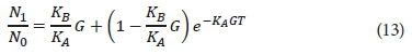
Bratby et al. (1977) proposed a model to describe the flocculation process in a static system considering that the particle concentration in the liquid mass is proportional to the turbidity, i.e., initial and final values of particle concentration (n₀ and n₁, respectively) were replaced by initial and final values of turbidity (N₀ and N₁, respectively). This model was based on Argaman (1968) and Argaman and Kaufman (1970)'s model (using it integro-differential form instead it original discrete form), and is presented in Eq. 12. It is important to emphasize that models proposed by Argaman (1968), Argaman and Kaufman (1970) and Bratby et al. (1977) were experimentally verified by Libânio et al. (1996) and Moruzzi and Oliveira (2012).

Alternatively:

In addition to the models previously mentioned, there are flocculation models in the literature based on fractal dimensions, among other parameters (Son and Hsu, 2008; Weber-Shirk and Lion, 2010; Cottereau et al., 2014; Sithebe Nomcebo and Nkhalambayausi Chirwa Evans, 2016). These models are considered more complex due to their high number of parameters and/or the great effort necessary to obtain them. Although such models have great importance in flocculation studies, they will not be detailed in this work. In this study, only global parameters of the process will be used (G, T, N₀ and N₁).

It is important to emphasize that, in all presented models, the influence of retention time in the flocculation process was not appropriately considered when the retention time is small. For example, Oliveira and Teixeira (2017), in their experimental work, present 7 flocculation units with retention times lower than 12 s, and with high efficiency. In this context, this paper proposes a flocculation model that appropriately considers the influence of retention time in the flocculation process to obtain a more adherent model when applied to low retention time units.

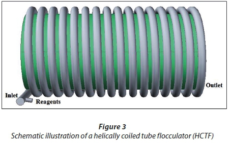
Among several flocculation units with low retention time, the helically coiled tube flocculators (HCTFs) have been gaining prominence in scientific research (Gregory, 1981; Grohmann et al., 1981; Vigneswaran and Setiadi, 1986; Al-Hashimi and Ashjyan, 1989; Elmaleh and Jabbouri, 1991; Thiruvenkatachari et al., 2002; Carissimi and Rubio, 2005; Silveira et al., 2009; Vaezi et al., 2011; Sartori et al., 2015; Oliveira and Teixeira, 2017a, b). Retention times verified in HCTFs are considerably lower than retention times verified in conventional flocculation units (such as baffled flocculation units). For example, Grohmann et al. (1981) presented a flocculation unit that promotes the formation of micro-flocs with a retention time equal to 14 s (about 0.78% of the retention time in a conventional unit) and reduced the final turbidity to 5% of the initial turbidity after 30 s (about 1.67% of the retention time in a conventional unit). HCTFs use hydraulic energy of the liquid helical flow to disperse flocculation reagents and promote collisions between particles to form flocs. These aspects provide a compact, and low-cost flocculation unit with high efficiency. Based on these characteristics, HCTFs will be used in this study as a proof flocculation unit to calibrate/validate the proposed model.

 

MATERIALS AND METHODS

This section describes the experimental apparatus applied to all configurations to obtain values of initial turbidity (N₀), final turbidity (N₁) and root mean square of the unit's velocity gradient (G), used in model calibration (as described in Results and Discussion section). This section is divided into 3 parts: first, reactor set-up is detailed. After that, the experimental modelling apparatus and procedures are shown and described. Finally, the main flocculation parameters used in this research are presented.

Reactor set-up

24 HCTFs configurations were tested and their characteristics are described in Table 1, where d is the tube diameter, D is the curvature diameter, p is the distance between consecutive passes divided by 2π and L is the HCTF length.

All HCTFs were tested under 2 different flow rates: HCTFs from No. 1 to No. 16 were tested under 1 and 2 L/min, and HCTFs from No. 17 to No. 24 were tested under 2 and 4 L/min, totalling 48 configurations. The set of HCTFs with the same values of d, D and p belong to the same arrangement. Variation of HCTF length was performed to vary retention time. Therefore, HCTFs from No. 1 to No. 8 belong to Arrangement I, HCTFs from No. 9 to No. 16 belong to Arrangement II and HCTFs from No. 17 to No. 24 belong to Arrangement III. All configurations were based on the experimental apparatus of Oliveira and Teixeira (2017).

Experimental modelling apparatus and procedures

The experimental apparatus used in this research is shown in Fig. 2, based on a complete cycle of the clarification system. It is composed of: a reservoir of synthetic water, a flow meter (flow controllers), dosing pumps of chemical reagents, pressure gauge connected at flocculator's input and output sections, flocculator, decanter system (settling tank) and drain to the final disposal of the fluid used in the search.

 

 

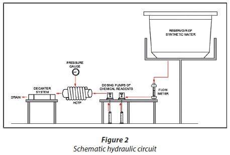
Initially, water is pumped and mixed with clay (bentonite), resulting in a synthetic water. Synthetic water was prepared in a controlled area to ensure that its main characteristics (turbidity, pH and temperature) were kept constant in all tests. A mixer operates continuously to ensure uniformity in synthetic water characteristics, with pH and temperature values approximately equal to 6.0 and 22°C, respectively. At the end of mixing, the effluent had an average turbidity of 50 UT, considered as initial turbidity value in all tests. After that, the flow rate was measured by a flow meter, the coagulant (aluminium sulphate, to cause destabilization of the particles, with a concentration of 43.85% and absolute density of 1.31 g/cm³) and the alkalizing agent (sodium hydroxide, for pH adjustment) are added by the dosing pumps located upstream of the flocculator. The aluminium sulphate dosing pump was a LMI Milton Roy P153-398Ti and the sodium hydroxide dosing pump was LMI Milton Roy P123-358Ti. Aluminium sulphate and sodium hydroxide concentrations were obtained through a coagulation diagram considering a turbidity removal efficiency equal to 80%, resulting in a concentration values equal to 40 mg/L of aluminium sulphate solution and 50 mg/L of sodium hydroxide. After the addition of these chemicals, the fluid passes through the flocculator (where manometers were used to measure head loss in all tests) and goes to the settling tank, where sample collection is made to determine the final turbidity. The final disposal of the fluid is made at the end drain. The experimental uncertainty based on instrumental uncertainty was 10%. Particle size and concentration are reduced enough to guarantee that they can follow streamlines in the unit. HCTF (Fig. 3) consists of a transparent and flexible polyvinyl chloride hose (PVC hose), coiled in a rigid PVC pipe. The hose used has a smooth internal surface with synthetic yarn reinforcement with high tenacity to ensure that there are no changes in the cross section along the reactor.

 

 

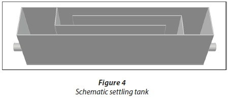
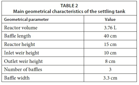
To ensure that the geometric and hydraulic features of the decanter do not influence the final turbidity removal efficiency of the process, a single decanter (with the same flow rate) was used in all experiments, keeping the sedimentation velocity constant, and uniformly influencing the clarification process. For this, the decanter was projected based on geometric and hydraulic parameters of a standard unit, with average values of reactor diameter, reactor length, and flow rate. The decanter design was based on retention time, flow velocity and input/output devices, following the methodology described by Edzwald (2011). The material used for the outside walls was polystyrene and the baffles were built with plastic sheets of 1.5 mm thickness. Figure 4 shows the schematic settling tank and Table 2 shows its main geometrical characteristics.

 

 

 

 

The flow rate inside the decanter was kept constant and equal to 0.3 L/min in all tests, to ensure that the decanter's characteristics do not influence the HCTFs' results. Due to this aspect, a system of fluid disposal connected to a rotameter was used, allowing for flow rate control. Samples were collected after a time equal to 3 times the decanter retention time, to ensure that the flow in the unit was in a steady state. The average sedimentation velocity used in all tests was 0.21 cm/s, according to Edzwald (2011).

Main flocculation parameters

The initial and final values of turbidity were obtained through a Hach model 2100 P turbidimeter, with resolution equal to 0.01 NTU and accuracy of ± 2%. Turbidity values were measured immediately after the sampling, avoiding changes in the fluid characteristics. In this work, a synthetic water was produced in a controlled environment with controlled characteristics (as described previously), making the use of a turbidity parameter sufficient for the analysis. It is important to emphasize that the isolated use of a turbidity parameter is not recommended in the analysis of natural water, since other parameters are necessary to characterize the process.

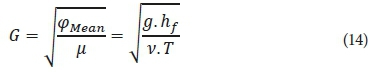
G values were obtained from Eq. 14, presented in Camp (1955), where G is given as a function of kinematic viscosity of the fluid (ν), head loss (h_f) and retention time (T).

Retention time was obtained through the ratio of HCTF volume to the flow rate.

 

RESULTS AND DISCUSSION

This section is divided into three parts: first, the mathematical aspects of the proposed model are detailed. After that, the model's coefficient calculation method is described (model calibration aspects). Finally, numerical results obtained with the proposed model are presented and a comparison with other commonly used models is performed.

Mathematical modelling aspects

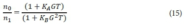
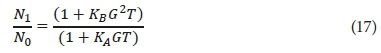
The flocculation model proposed by Argaman (1968) and Argaman and Kaufman (1970) is presented again in Eq. 15, as a function of aggregation and breakup coefficients (K_A and K_B, respectively), the root mean square of the unit's velocity gradient (G) and retention time (T).

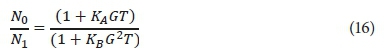
Considering that the concentration of primary particles is proportional to turbidity, as seen in Bratby et al. (1977), initial and final values of particle concentration (n₀ and n₁, respectively) can be replaced by initial and final values of turbidity (N₀ and N₁, respectively) - Eq. 16:

Alternatively:

In order to estimate particle variation in the liquid mass (dn₁/dT, alternatively, dN₁/dT) during the flocculation process, Bratby et al. (1977) reorganized the differential equation of Argaman (1968) and Argaman and Kaufman's (1970) model, presenting one term related to the aggregation process and one term related to the break-up process, as shown in Eq. 18.

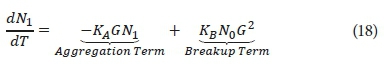
An accurate analysis performed in Eq. 18, especially in the aggregation term, allows us to verify that this term depends on the number of flocs existing in the flocculation unit at time T (N₁), representing the collision between a discrete particle and a floc. However, in flocculation units with lower retention times, the flocculation process is more sensitive to the time (T) than to the number of flocs previously existing in the flocculation unit (N₁). Therefore, the model presented in Eq. 18 should be adjusted to Eq. 19:

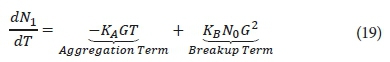
The necessary development is presented below, and the resulting flocculation model is presented in Eq. 20.

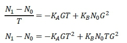
Dividing the previous equation by N₀, results:

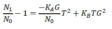
Isolating N₁/N₀, results:

Equation 20 allows us to determine turbidity removal in a flocculation unit (N₁/N₀) as a function of K_A and K_B constants, the root mean square of the unit's velocity gradient (G) and retention time (T).

Model coefficient calculation (model calibration aspects)

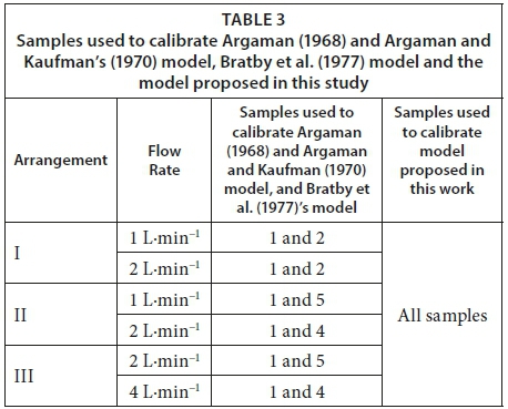
The determination of constants K_A and K_B of Bratby et al. (1977)'s model - Eq. 13 - was performed with two samples for each combination of arrangement and flow rate, according to the method described in Brito (1998). The first step of this method consists of applying the values of maximum efficiency (at the lower retention time) in the derivative of Eq. 13, making dN₁/dt = 0, and obtaining K_B/K_A. After that, a second point was necessary to obtain both separately; to standardize the calibration process, the first HCTF for each arrangement was chosen.

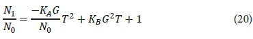
The determination of constants K_A and K_B of Argaman (1968) and Argaman and Kaufman's (1970) model - Eq. 17 - and of the proposed model - Eq. 20 - was performed from overestimate least squares method application to the samples (Verhaegen and Verdult, 2007). Rearranging the terms of Eqs 17 and 20 as a function of constants K_A and K_B, results in Eqs 21 and 22, respectively:

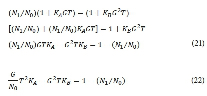
Equations 21 and 22 can be expressed in a matrix form, considering the samples available for each arrangement (Table 1), resulting in a linear system shown in Eqs 23 and 24, respectively. The general solution of a linear system is given by Eq. 25.

The obtainment of K_A and K_B constants to Argaman (1968) and Argaman and Kaufman's (1970) model - Eq. 17 - was performed with 2 samples for each combination of arrangement and flow rate. The number of samples was defined to guarantee the convergence of the method with the same number of samples for all arrangements. The obtainment of K_A and K_B constants for the proposed model - Eq. 20 - was performed with all samples available for each combination of arrangement and flow rate. Samples used in each case are shown in Table 3. In all cases, MATLAB R2012b was used to fit the models.

 

 

Numerical results

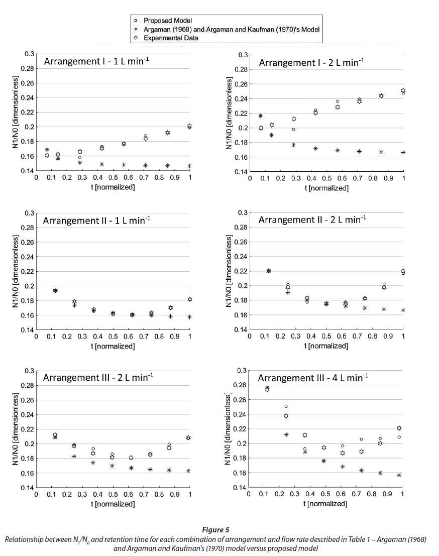
Maximum and average absolute percentage deviation values, obtained between experimental data and Argaman (1968) and Argaman and Kaufman (1970) model, Bratby et al. (1977) model and the model proposed in this study, are shown in Table 4. Figures 5 and 6 show the relationship between N₁/N₀ (representing the turbidity removal) and retention time for each combination of arrangement and flow rate described in Table 1, comparing Argaman (1968) and Argaman and Kaufman's (1970) model with the proposed model (Fig. 5) and the model of Bratby et al. (1977) model with the proposed model (Fig. 6).

From Fig. 5, Fig. 6 and Table 4 it is possible to verify that the model proposed in this study presents results more adherent to the physical process, when compared with Argaman (1968) and Argaman and Kaufman's (1970)'s model and that of Bratby et al. (1977), for all arrangements/flow rates. In the best case (Arrangement II - 1 L·min⁻¹), maximum and average absolute percentage deviations obtained using the model proposed in this study were 1.4% and 0.4%, respectively. The major difference occurred with Arrangement III - 4 L·min⁻¹, whose maximum and average absolute percentage deviations obtained using the model proposed in this study were 9.5% and 6.1%, respectively. Maximum and average absolute percentage deviations obtained using the model proposed in this study were less than or equal to 10% (experimental uncertainty, described in 'Materials and Methods') for all cases. However, maximum and average absolute percentage deviations obtained using Argaman (1968) and Argaman and Kaufman's (1970) model reach 32.9% and 19.6%, respectively (Arrangement I - 2 L·min⁻¹). With the model of Bratby et al. (1977), maximum and average absolute percentage deviations reach 155.6% and 36.7%, respectively (Arrangement I - 1 L·min⁻¹). Values of the determination coefficient were increased, varying between 0.76 and 0.99 using the model proposed in this study. With Argaman (1968) and Argaman and Kaufman's (1970) model, values of the determination coefficient varied between 0.19 and 0.70. With the model of Bratby et al. (1977), values of the determination coefficient varied between 0.16 and 0.77. Furthermore, two parameters were used to measure the quality of the model: sum of squared errors (SSE) and root mean square error (RMSE). The values of these parameters decreased when the model proposed in this study is compared with the other's evaluated models. Additionally, the asymptotic characteristic observed in Argaman (1968) and Argaman and Kaufman's (1970) model (Fig. 5) and the model of Bratby et al. (1977) (Fig. 6), differs significantly from the decreasing-rising behaviour experimentally verified. This fact does not occur with the model proposed in this study, which presents a decreasing-rising behaviour, like that of the experimental data.

In the end, it is important to emphasize that dynamic similarity studies are necessary to allow the application of HCTFs at real-world large scale. This is necessary since the experiments performed in this work used prototypes, with low flow rate values.

 

CONCLUSIONS

This paper began by exploring the main mathematical models for orthokinetic interactions proposed in the literature. In the performed review, most of the presented models do not appropriately consider the influence of retention time in flocculation processes, with this assumption valid only for units with high retention times. Thus, this paper proposed a new flocculation model, adherent to flocculation units with low retention times, and able to appropriately consider the influence of retention time in the flocculation process.

Among several flocculation units with low retention time, HCTFs have been gaining prominence in scientific research, due to their compact size, low cost, and high efficiency. Based on these characteristics, HCTFs were used in this study as a proof flocculation unit to calibrate/validate the proposed model.

In the proposed model, a substitution of the term referring to the number of flocs previously existing in the flocculation unit for the term referring to the time was performed, being relevant in flocculation units with low retention time.

The model proposed in this study presented results more adherent to the physical process (using 24 HCTFs with 2 flow rates, totalling 48 configurations), when compared with commonly used models, for all arrangements/flow rates. In the best case, maximum and average absolute percentage deviations obtained using the model proposed were 1.4% and 0.4%, respectively. The major differences were 9.5% and 6.1%, respectively, lower than the experimental uncertainty. Maximum and average absolute percentage deviations obtained with reference models reach 155.6% and 36.7%, respectively.

Furthermore, the asymptotic characteristic observed in the reference models differs significantly from the decreasing-rising behaviour experimentally verified. This fact does not occur with the model proposed in this study, which presents a decreasing-rising behaviour, like the experimental data.

 

ACKNOWLEDGMENTS

The authors would like to acknowledge the institutional and financial support from Federal Institute of Espírito Santo (IFES), Federal University of Espírito Santo (UFES), Coordination for the Improvement of Higher Education Personnel (CAPES) and National Counsel of Technological and Scientific Development (CNPq).

 

REFERENCES

AGUNBIADE MO, POHL CH and ASHAFA AOT (2016) A review of the application of bioflocculants in wastewater treatment. Pol. J. Environ. Stud. 25 (4) 1381-1389. https://doi.org/10.15244/pjoes/61063        [ Links ]

AL-HASHIMI MAI and ASHJYAN ASK (1989) Effectiveness of helical pipes in the flocculation process of water. Filtration Sep. J. 26 (6) 422-429.         [ Links ]

ARGAMAN Y (1968) Turbulence in orthokinect flocculation. Thesis, University of California, Berkeley.         [ Links ]

ARGAMAN Y and KAUFMAN WJ (1970) Turbulence and flocculation. J. Sanitary Eng. Div.. Proc. Am. Soc. Civ. Eng. 96 (SA 2) 223-241.         [ Links ]

BRATBY J, MILLER MW and MARAIS GR (1977) Design of flocculation systems from batch test data. Water SA 3 (4) 173-182.         [ Links ]

BRITO SA (1998) Influence of sedimentation velocity on aggregation and rupture coefficients determination during flocculation (in Portuguese). University of São Paulo, São Paulo.         [ Links ]

CAMP TR (1955) Flocculation and flocculation basins. ASCE Trans. 120 1-16.         [ Links ]

CAMP TR and STEIN PC (1943) Velocity gradients and internal work in fluid motion. J. Boston Soc. Civ. Eng. 30 (4) 219-237.         [ Links ]

CARISSIMI E and RUBIO J (2005) The flocs generator reactor - FGR: a new basis for flocculation and solid-liquid separation. Int. J. Miner. Process. 75 237-247. https://doi.org/10.1016/j.minpro.2004.08.021        [ Links ]

COTTEREAU R, ROCHINHA FA and COUTINHO ALGA (2014) Comparison of two parameterizations of a turbulence-induced flocculation model through global sensitivity analysis. Continental Shelf Res. 85 85-95. https://doi.org/10.1016/j.csr.2014.07.002        [ Links ]

EDZWALD JK (2011) Water Quality & Treatment: A Handbook on Drinking Water. McGraw-Hill, New York.         [ Links ]

ELMALEH S and JABBOURI A (1991) Flocculation energy requirement. Water Res. 25 (8) 939-943. https://doi.org/10.1016/0043−1354(91)90141-C        [ Links ]

FAIR GM and GEMMELL RS (1964) A mathematical model of coagulation. J. Colloid Sci. 19 360-372. https://doi.org/10.1016/0095-8522(64)90037-6        [ Links ]

GREGORY J (1981) Particle interactions in flowing suspensions. Adv. Colloid Interf. Sci. 17 (1) 149-160. https://doi.org/10.1016/0001-8686(82)80016-X        [ Links ]

GROHMANN A, REITER M and WIESMANN U (1981) New flocculation units with high efficiency. Water Sci. Technol. 13 (11/12) 567-573.         [ Links ]

HARRIS HF, KAUFMAN WJ and KRONE RB (1966) Orthokinect flocculation in water purification. J. San. Eng. Div. Proc. ASCE 92 (SA6) 95-111.         [ Links ]

HUDSON HE (1965) Physical aspects of flocculation. J. Am. Water Works Assoc. 57 (7) 885-892. https://doi.org/10.1002/j.1551-8833.1965.tb01476.x        [ Links ]

KHANNOUS L, ABID D, GHARSALLAH N, KECHAOU N and BOUDHRIOUA MIHOUBI N (2011) Optimization of coagulation-flocculation process for pastas industry effluent using response surface methodology. Afr. J. Biotechnol. 10 (63) 13823-13834. https://doi.org/10.5897/AJB11.1142        [ Links ]

LIBÂNIO M, PADUA VLD and BERNARDO LD (1996) Argaman & Kaufman's model evaluation in the flocculation units performance estimation applied to the water treatment supply (in Portuguese). San. Environ. Eng. 1 (2).         [ Links ]

MA J, FU K, FU X, GUAN Q, DING L, SHI J, ZHU G, ZHANG X, ZHANG S and JIANG L (2017) Flocculation properties and kinetic investigation of polyacrylamide with different cationic monomer content for high turbid water purification. Sep. Purif. Technol. 182 (Supplement C) 134-143. https://doi.org/10.1016/j.seppur.2017.03.048        [ Links ]

MACEDA-VEIGA A, WEBSTER G, CANALS O, SALVADÓ H, WEIGHTMAN AJ and CABLE J (2015) Chronic effects of temperature and nitrate pollution on Daphnia magna: Is this cladoceran suitable for widespread use as a tertiary treatment? Water Res. 83 (Supplement C) 141-152. https://doi.org/10.1016/j.watres.2015.06.036        [ Links ]

MORUZZI R and OLIVEIRA S (2012) Mathematical modeling and analysis of the flocculation process in chambers in series. Bioprocess Biosyst. Eng. 36 (3) 357-363. https://doi.org/10.1007/s00449-012-0791-4        [ Links ]

MUDHIRIZA T, MAPANDA F, MVUMI BM and WUTA M (2015) Removal of nutrient and heavy metal loads from sewage effluent using vetiver grass, Chrysopogon zizanioides (L.) Roberty. Water SA 41 (4) 457-463. https://doi.org/10.4314/wsa.v41i4.04        [ Links ]

OLIVEIRA DS and TEIXEIRA EC (2017a) Experimental evaluation of helically coiled tube flocculators for turbidity removal in drinking water treatment units. Water SA 43 (3) 378-386. https://doi.org/10.4314/wsa.v43i3.02        [ Links ]

OLIVEIRA DS and TEIXEIRA EC (2017b) Hydrodynamic characterization and flocculation process in helically coiled tube flocculators: an evaluation through streamlines. Int. J. Environ. Sci. Technol. 14 (12) 2561-2574. https://doi.org/10.1007/s13762-017−1341-z        [ Links ]

SARTORI M, OLIVEIRA DS, TEIXEIRA EC, RAUEN WB and REIS NC (2015) CFD modelling of helically coiled tubes for velocity gradient assessment. J. Braz. Soc. Mech. Sci. Eng. 37 (1) 187-198. https://doi.org/10.1007/s40430-014-0141-3        [ Links ]

SHAIKH SMR, NASSER MS, HUSSEIN I, BENAMOR A, ONAIZI SA and QIBLAWEY H (2017) Influence of polyelectrolytes and other polymer complexes on the flocculation and rheological behaviors of clay minerals: A comprehensive review. Sep. Purif. Technol. 187 (Supplement C) 137-161. https://doi.org/10.1016/j.seppur.2017.06.050        [ Links ]

SILVEIRA AND, SILVA R and RUBIO J (2009) Treatment of acid mine drainage (AMD) in South Brazil: comparative active processes and water reuse. Int. J. Miner. Process. 93 103-109. https://doi.org/10.1016/j.minpro.2009.06.005        [ Links ]

SITHEBE NP and CHIRWA EMN (2016) Mechanistic flocculation model incorporating the fractal properties of settling particles. J. Environ. Eng. 142 (7) 04016027. https://doi.org/10.1061/(ASCE)EE.1943-7870.0001096        [ Links ]

SMOLUCHOWSKI M (1917) Versuch einer mathematischen theorie der koagulationskinetik kolloider lösungen. Z. Phys. Chem. 92 129-168        [ Links ]

SON M and HSU T-J (2008) Flocculation model of cohesive sediment using variable fractal dimension. Environ. Fluid Mech. 8 (1) 55-71. https://doi.org/10.1007/s10652-007-9050-7        [ Links ]

THIRUVENKATACHARI R, NGO HH, HAGARE P, VIGNESWARAN S and AIM RB (2002) Flocculation-cross-flow microfiltration hybrid system for natural organic matter (NOM) removal using hematite as a flocculent. Desalination 147 (1) 83-88. https://doi.org/10.1016/S0011-9164(02)00580-5        [ Links ]

UGBENYEN A and OKOH A (2014) Characteristics of a bioflocculant produced by a consortium of Cobetia and Bacillus species and its application in the treatment of wastewaters. Water SA 40 (1) 139-144. https://doi.org/10.4314/wsa.v40i1.17        [ Links ]

VAEZI F, SANDERS RS and MASLIYAH JH (2011) Flocculation kinetics and aggregate structure of kaolinite mixtures in laminar tube flow. J. Colloid Interf. Sci. 355 96-105. https://doi.org/10.1016/j.jcis.2010.11.068        [ Links ]

VERHAEGEN M and VERDULT V (2007) Filtering and System Identification: A Least Squares Approach, Cambridge University Press, Cambridge. https://doi.org/10.1017/CBO9780511618888        [ Links ]

VIGNESWARAN S and SETIADI T (1986) Flocculation study on spiral flocculator. Water Air Soil Pollut. 29 (2) 165-188 https://doi.org/10.1007/BF00208407        [ Links ]

WATANABE Y (2017) Flocculation and me. Water Res. 114 (Supplement C) 88-103. https://doi.org/10.1016/j.watres.2016.12.035        [ Links ]

WEBER-SHIRK ML and LION LW (2010) Flocculation model and collision potential for reactors with flows characterized by high Peclet numbers. Water Res. 44 (18) 5180-5187. https://doi.org/10.1016/j.watres.2010.06.026        [ Links ]

YANG Z, YANG H, JIANG Z, HUANG X, LI H, LI A and CHENG R (2013) A new method for calculation of flocculation kinetics combining Smoluchowski model with fractal theory. Colloids Surf. A: Physicochem. Eng. Asp. 423 11-19. https://doi.org/10.1016/j.colsurfa.2013.01.058        [ Links ]

 

 

Received 20 December 2017
Accepted in Revised form 12 December 2018.

 

 

* To whom all correspondence should be addressed. e-mail: danieli@ifes.edu.br

 

 

APPENDIX

 

Appendix - Click to enlarge