ORIGINAL ARTICLES

 

Applications of the PyTOPKAPI model to ungauged catchments

 

 

Zeinu Ahmed Rabba^*; BS Fatoyinbo; Derek D Stretch

Centre for Research in Environmental, Coastal & Hydrological Engineering, School of Engineering, University of KwaZulu-Natal, Durban 4041, South Africa

 

 

---

ABSTRACT

Many catchments in developing countries are poorly gauged/totally ungauged which hinders water resource management and flood prediction in these countries. This study explored the application of the PyTOPKAPI model to South African (Mhlanga) and Ethiopian (Gilgel Ghibe) case study catchments to test its suitability for simulating stream flows from ungauged catchments. The aim is to extend the model application to poorly gauged/totally ungauged catchments in developing countries. The model uses digital elevation data and other spatial data sources to set up the model parameters and the forcing files. To generate reliable stream flows, models generally need to be calibrated, which typically relies on the availability of reliable stream flow data. We show how application of simple lumped models for average runoff ratios, such as that proposed by Schreiber in 1904, can be used as an alternative to detailed calibration with gauged flows. This approach seems to be new; and we show how the proposed method, together with the PyTOPKAPI model, can be used to predict runoff responses in ungauged catchments for water resource applications and flood forecasting in developing countries.

Keywords: PyTOPKAPI, Schreiber formula, streamflow, runoff ratio, South Africa, Ethiopia

---

 

 

INTRODUCTION

Flooding is one of the natural disasters that can lead to loss of life and property. Accurate streamflow modelling and forecasting is therefore a key issue in hydrology for flood management (Kamruzzaman et al., 2014; Saeidifarzad et al., 2014; Zhao et al., 2014; Wu and Lin, 2015; Liu et al., 2017) and is also vital for water resource applications (Blöschl, 2013; Ries III, 2007; Sanborn and Bledsoe, 2006). However, estimation of streamflow time series in ungauged catchments remains a challenge. Early attempts at estimating streamflow from ungauged catchments employed calibrated model parameters from nearby gauged catchments where streamflow data were available. However, the modelled streamflow from ungauged catchments may have errors when basin characteristics such as geography, land use and soil type are significantly different from those of gauged catchments (Jeon et al., 2014; Vis et al., 2015). This issue of streamflow predictions in ungauged catchments remains an area of active research. The present study demonstrates the implementation of the PyTOPKAPI model (Sinclair and Pegram, 2012; Vischel et al., 2008) in South African (Mhlanga) and Ethiopian (Gilgel Ghibe) ungauged catchments, for streamflow simulation. However, since the two catchments are poorly gauged in a sense that there were rainfall data but little/no stream flow data, it is difficult to calibrate the model for reliable streamflow simulation from the catchments. In this study, we investigate the use of the runoff-ratio formula proposed by Schreiber in 1904 (Arora, 2002; Fraedrich, 2010; Fraedrich and Sielmann, 2011; Fraedrich et al., 2015) to calibrate the PyTOPKAPI model, as an alternative to detailed model calibration procedures, which can be used when there is plentiful data. This approach seems to be a new method proposed in this work as an alternative model calibration procedure for streamflow simulation from ungauged catchments. In Schreiber's work, the runoff-ratio is the (time-averaged) ratio of volume of runoff to volume of rainfall in a catchment. It illustrates the average excess rainfall for a catchment (Fraedrich et al., 2015). Consequently, the runoff ratios were computed from the simulated stream flows and the rainfall data of the study catchments. The model was then calibrated by comparing the simulated runoff-ratio with that predicted by the Schreiber's formula. We found that the calibrated PyTOPKAPI model generated a realistic daily streamflow time series over the catchments.

The first section of this paper introduces the methods used while the second outlines the results, with discussion focusing on the output of model calibration and validation. The last section presents concluding remarks and recommendations.

 

MATERIALS AND METHODS

Description of the case study catchments

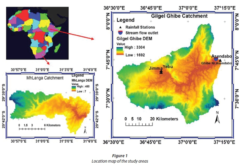
In this study, the PyTOPKAPI model was implemented on South African (Mhlanga) and Ethiopian (Gilgel Ghibe) ungauged catchments. These two catchments are geographically located in different hydrological regimes; the Gilgel Ghibe is found at a high altitude in a wet tropical zone while the Mhlanga catchment drains an area that is lower in elevation in a temperate zone. The two catchments are briefly described below.

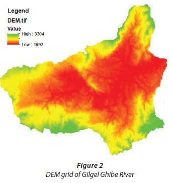
The Gilgel Ghibe catchment (Fig. 1) feeds a tributary of the Ghibe River (EthioVisit.com, 2016) with a drainage area of 2 943 km², and is located in the southwest of Ethiopia extending between longitudes 36°31'04.91'' E and 37°13'31.07'' E, and latitudes 7°20'01.58'' N and 7°59'15.32'' N. It is characterized by high-relief hills and mountains with elevations between 1 692 and 3 304 m amsl. The basin's land use is composed of fallow lands (29.6%), forestlands (13.5%), woodlands (28.8%), grasslands (15.7%), and bush and shrublands (13.1%), and urban and water (0.3%) (Negash, 2012). The climate of the catchment is sub-tropical, humid, and warm to hot. The average monthly temperature is 19°C, with minimum of 2.5°C, and maximum of 32.6°C. Rainfall follows a mono-modal pattern, occurring mainly between June and September. These summer rains account for 50-80% of annual rainfall totals over the catchment (Demissie, 2013). The mean annual rainfall of the catchment is 1 456 mm, and the mean annual discharge is 52.7 m³/s (565 mm, calculated from observed streamflow data). The mean annual evapotranspiration of the catchment is about 1 306 mm (obtained from the computed potential evapotranspiration). The dominant soil types in the basin are clay and clay-loam, with a very small portion of sandy clay-loam and loam (HWSD) (FAO/IIASA/ISRIC/ISS-CAS/JRC, 2012).

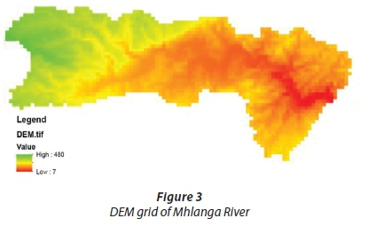
Mhlanga catchment (Fig. 1) is a typical small ungauged catchment in South Africa having a catchment area of about 80 km², and is found in the U30B quaternary catchment area downstream of Mdloti Hazelmere Dam (Midgley et al., 1994; Zietsman, 2003; Middleton and Bailey, 2005) and provides runoff directly into the Indian Ocean, to the north of Durban, KwaZulu-Natal (Zietsman, 2003). Geographically, it is located between 29°39'00'' and 29°42'09'' S, and 30°57'00'' and 31°06'00'' E, on the east coast of South Africa, with an average slope of 0.6%. It has a mean annual precipitation of about 1 000 mm, mean annual runoff of 0.4 nrVs (157 mm) (Zietsman, 2003; Stretch and Zietsman, 2004) and a mean annual evapotranspiration of 1 792 mm (obtained from the computed potential evapotranspiration).

Description of the PyTOPKAPI model

The PyTOPKAPI model is an improved version of the earlier TOPKAPI model (Sinclair and Pegram, 2012; Sinclair and Pegram, 2013a). TOPKAPI is the acronym of: TOPographic Kinematic Approximation and Integration, and is a physically-based, fully-distributed rainfall-runoff model applicable at different spatial scales, ranging from the hill slope to the catchment scale, while keeping the physical meaning of the model parameters (Liu and Todini, 2002; Liu et al., 2008). The model is based on the lumping of a kinematic wave assumption (Vischel et al., 2008) for flows in the soil, over the land and in the channel (Ciarapica and Todini, 2002), and results in converting the rainfall-runoff and runoff routing processes into three 'structurally-similar' zero-dimension non-linear reservoir differential equations describing the different hydrological and hydraulic processes (Liu and Todini, 2002).

A correct integration of the differential equations provides a relatively scale-independent physically-based model which preserves the physical meaning of the model parameters. The geometry of the catchment is described by the pixels of a digital elevation model (DEM), over which the equations are integrated to feed into a cascade of non-linear reservoirs. It is assumed that the non-linear cascade aggregates into a unique non-linear reservoir at the basin level whose parameter values can be estimated directly from the small-scale values without losing the physical meaning of them (Liu and Todini, 2002; Vischel et al., 2008). Each grid cell of the DEM is assigned a value for each of the physical characteristics represented in the model. The flow directions and slopes are evaluated starting from the DEM, according to a neighbourhood relationship based on the principle of minimum energy; namely, the maximum elevation difference that takes into account the links between the active cell and the four surrounding cells connected along the edges. The active cell is assumed to be connected with a single downstream cell, while it can receive from up to three upstream contributing cells (Ciarapica and Todini, 2002; Liu and Todini, 2002).

The TOPKAPI model consists of 5 main modules; namely, soil, overland, channel, evapotranspiration, and snow modules (Liu and Todini, 2002; Liu et al., 2008). The first 3 modules take the form of non-linear reservoir equations controlling the horizontal flows. This mechanism plays a fundamental role in the model, both as a direct contribution to the flow into the channel network and as a factor regulating the soil moisture balance, particularly with regard to the dynamics of the saturated areas. Overland flow is generated by the excess rainfall on the different saturated cells while the total runoff (surface and sub-surface) is then drained by the drainage network. In the current PyTOPKAPI modelling, evapo-transpiration was introduced directly as an input to the model, while the snow module component was totally ignored since there are no snowfalls in the study catchments. In the flow simulation, on the basis of the soil condition and actual evapotranspiration, the precipitation onto the catchment is divided into direct runoff and infiltration, which reflects the nonlinear relationship between the soil water storage and the saturated contributing area in the basin. The infiltration and direct runoff are input into the soil reservoir and surface reservoir, respectively. Outflows from the two reservoirs as interflow and overland flow are then drained into the channel reservoir to form the channel flow (Liu and Todini, 2002).

The improved PyTOPKAPI model is coded in Python programming language and accessed directly through an interactive Python environment. It is open-source with BSD license, and runs on most popular operating systems (Sinclair and Pegram, 2012). The model was previously tested on the Liebenbergsvlei gauged catchment in South Africa to simulate river discharge at 6-h time-steps and showed good performance (Vischel et al., 2008).

PyTOPKAPI model input data

Basically, the PyTOPKAPI model input comprises gridded data including: (i) a digital elevation model (DEM); (ii) a soil type; (iii) a land use; and (iv) hydro-meteorological data, such as rainfall and temperature data. The observed streamflow data were also utilized for testing the suitability of the calibration approach. These data are briefly described hereunder.

Digital elevation model (DEM)

The SRTM DEM (Jarvis et al., 2008) was used for the current study. The resolutions of the DEM were set to 1 km for Gilgel Ghibe and 500 m for Mhlanga (Figs 2 and 3). These resolutions have been respectively adopted for all the terrain maps.

 

 

 

 

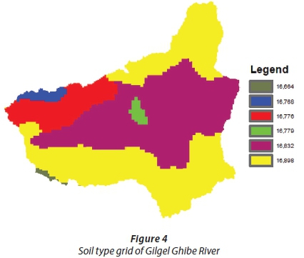
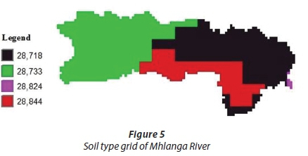
Soil type data

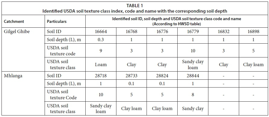
These data were acquired from the Harmonized World Soil Database (FAO/IIASA/ISRIC/ISS-CAS/JRC, 2012). The HWSD is composed of raster image files and a linked attribute data file. The grids contain the dominant soil texture class for each of the 13 standard soil layers using the USDA soil texture class index by referring to the HWSD attribute table (Fischer et al., 2008). Table 1 shows the identified USDA soil texture class index and USDA soil texture class name and code for the Gilgel Ghibe and Mhlanga catchments. Figures 4 and 5 show the soil maps for the two catchments, respectively.

 

 

 

 

Land use

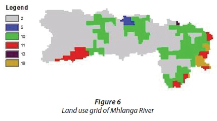
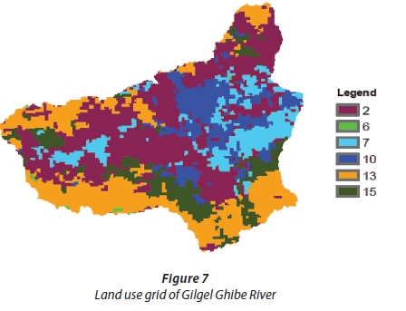
The land use maps were obtained from the United States Geological Survey (USGS) Global Land Cover Characterization (GLCC) database and are accessible through the WaterBase web page (UNU-INWEH, 2016). These maps are available in the form of tiles for each continent/region in two resolutions: the original at approximately 400 m (at the equator), and resampled versions at 800 m. For this study, the '400 m resolution' was used as it is finer. The PyTOPKAPI model requires the values of the Manning's coefficient for every grid cell for each land use class. These parameters were obtained from the land use gridded data from the USGS Land Use/Land Cover System Legend-Modified Level 2 (GLCC, 2008) and Manning's coefficient values used for various land cover classes in GeoSFM (Asante et al., 2008). Figures 6 and 7 show the land use grids of the two river catchments. Table 2 shows the identified land use classes and Manning's coefficient (n_o) values for the two catchments.

 

 

 

 

Hydro-meteorological data

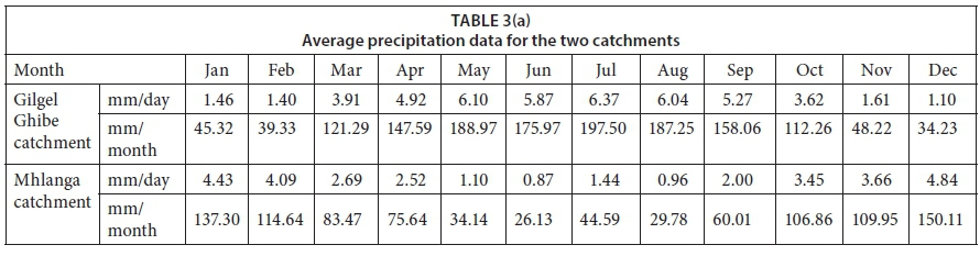
The available meteorological data for Gilgel Ghibe catchment comprised daily rainfall and temperature records from Jimma, Asendabo and Yebu weather stations (Fig. 1) for the period from 01/01/1986 to 31/12/2010 obtained from the Ethiopian National Meteorological Agency (ENMA). For the Mhlanga catchment, daily rainfall between 01/01/1980 and 31/10/2009 was obtained from the South African Weather Service (SAWS). Table 3(a) shows the average precipitation data for the two catchments. We also obtained daily streamflow data (19862010) at the Gilgel Ghibe outlet (Fig. 1) from the Ministry of Water, Irrigation and Electricity in Ethiopia. The Mhlanga catchment does not have any directly-observed streamflow data, so 30 years (1980-2009) of streamflow data for the neighbouring Mdloti River at the Hazelmere Dam gauging station was utilized.

Potential evapotranspiration (ETo)

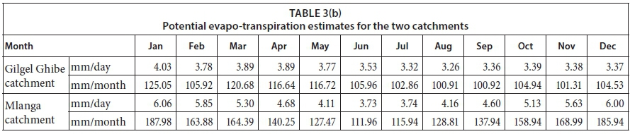
The ETo data used were obtained by taking the average value of ETo computed by the methods of Blaney-Criddle (Blaney and Criddle, 1962) and Thornthwaite (Thornthwaite, 1948; Thornthwaite and Mather, 1955) for Gilgel Ghibe catchment; and using the method of Blaney-Criddle (Blaney and Criddle, 1962) for Mhlanga catchment. Table 3(b) shows the computed ETo data for the two catchments.

PyTOPKAPI model set-up

The PyTOPKAPI rainfall-runoff modelling starts with preprocessing of the DEM and preparation of model input files, and then applies them in the model to simulate the streamflow data along the drainage system. The model was set up using the essential data described above for simulating stream flows. The model setup steps are briefly summarized below.

1. The DEM of the study areas were loaded to the GIS and were treated by pre-processors that help eliminate the false outlets and the sinks so that the flow direction and the basin closure cell are uniquely identified.

2. The stream network was generated by defining a threshold area that initiates a stream. In this case, 25 km² was used as 'Threshold area' to define the stream network as per the recommendation of Todini (Sinclair and Pegram, 2013b).

3. The location of the outlet was carefully selected and then the entire watershed of the respective catchment was delineated.

4. Similarly, the land use and the soil maps were loaded to GIS and then extracted by the defined watershed as a mask. The attribute table for each map was edited with the values of the literature parameters (Fischer et al., 2008).

5. Then, the different thematic maps (the GIS files to generate parameter files) were created.

6. Thereafter, cell parameters were generated and modified to eliminate zero slopes.

7. Next, the rainfall and the ETo data were prepared as the forcing files in HDF5 format.

8. Finally, the model simulated the streamflow time series for the simulation periods.

PyTOPKAPI model calibration

In principle, a physically-based model such as the PyTOPKAPI model should require no calibration since its parameters are estimated from catchment data such as morphology and hydraulic catchment properties, soil, vegetation, literature and experience (Coccia et al., 2009). Even though the PyTOPKAPI model is a physically-based model, it is of course subject to several uncertainties associated with the input data, and with approximations introduced by the scale of the parameter representations. For these reasons, Liu and Todini (2002) suggest that calibration of the parameters is still necessary for fine-tuning the model. Previous studies using the PyTOPKAPI model indicated that satisfactory model performance can be achieved by simple trial-and-error adjustment of grouped key parameters (Pegram et al., 2010) to match observed streamflow. This is not an option in the case of ungauged catchments. Thus, the use of the runoff-ratio formula proposed by Schreiber in 1904 (Fraedrich, 2010) was used as an alternative to detailed model calibration procedure. The runoff-ratio shows the percentage of precipitation that appears as runoff by taking other basin characteristics (e.g., soil, slope, vegetation) into account. It is a measure of the overall water balance of a basin and indicates how well the model is simulating the water balance of the basin (in an average sense) based on the primary input information (Fraedrich et al., 2015).

Schreiber analysed data for the annual mean discharge R versus the annual precipitation P of continental European river basins and fitted them to a polynomial curve a century ago. Looking at that curve, he developed the formula: R = P (e^-ETo/P) where ETo is potential evapotranspiration; and the expression (ETo/P) is defined as an aridity index 0 (Fraedrich, 2010; Fraedrich and Sielmann, 2011; Fraedrich et al., 2015). The functional form of Schreiber's formula is based on the aridity index 0, and is a reasonable first-order approximation of the actual evapotranspiration (ETa) (Arora, 2002; González-Zeas et al., 2012). Thus, it may be called an integrated runoff-ratio calculated using the functional form of the aridity index 0. The formula can also be extended to determine the ratio between the actual evapotranspiration (ETa) and the precipitation (P), through the water balance as shown below.

Water balance refers to the quantitative description of the hydrologic cycle. Empirical data from catchments all over the world indicate that the long-term water balance is primarily controlled by water supply (i.e., precipitation) and energy demand (i.e., potential evapotranspiration) (Zhang et al., 2015). Water is supplied by precipitation, and is balanced by runoff and evapotranspiration (Dooge, 1992; Fraedrich et al., 2015). Thus, the basic water balance can be expressed as:

from which, the evapotranspiration ratio is expressed as (Arora, 2002; Fraedrich et al., 2015)

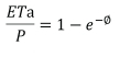
where Ø = ETo/P thereby yielding the value of the mean annual runoff (R) as a function of the aridity index and precipitation (P) (González-Zeas et al., 2012) that, lastly, gives the runoff-ratio as:

Accordingly, we used the above integrated Schreiber's runoff-ratio formula for computation of the runoff-ratios to calibrate the model. In this case, the monthly average ETo values are 109 mm and 149 mm; and the precipitation (P) values are 120 mm and 82 mm, for Gilgel Ghibe and Mhlanga catchments, respectively; from which the runoff-ratios were computed (Table 4).

 

 

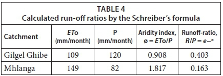
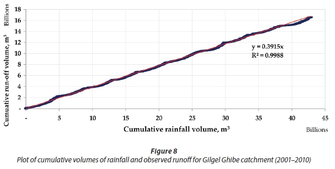
If observed streamflow data are available, the runoff-ratios can also be obtained from the plot of cumulative volume of precipitation versus the cumulative volume of observed discharge data. Thus, the runoff-ratio based on 10 years (2001-2010) of data for Gilgel Ghibe catchment was 39% (Fig. 8). The mean and the standard deviation of the data for Gilgel Ghibe are 1.57 mm and 1.248 mm, respectively. For Mhlanga catchment we used 15 years (1980-1994) of daily streamflow data from the neighbouring Mdloti station, the mean and standard deviation of which were 0.41 mm and 1.94 mm, respectively, for estimating the runoff-ratio in the region, which was 16%. The generally good agreement between the observed values and those predicted by the Schreiber runoff-ratio formula indicate that the Schreiber's formula can be used in these regions to predict average runoff-ratios for use in calibrating the PyTOPKAPI model.

Therefore, the model could effectively be calibrated by comparing the simulated runoff-ratio with the Schreiber's runoff-ratio. According to a sensitivity analysis conducted by researchers (Liu et al., 2005), the most sensitive model parameters controlling the runoff production are the soil depth L and the soil conductivity K, whereas the Manning roughness of channel n_cand overland n_gare the primary routing parameters. While calibrating the model, we also observed that the most sensitive model parameter was the saturated hydraulic conductivity K, followed by the soil depth L. These parameters are discussed below.

The first and the most sensitive parameter is K. It is the most important soil hydraulic parameter for flow in soil. Direct measurement of this parameter is 'very difficult, laborious, and costly' (Rawls et al., 1982 p. 1316) under field or laboratory conditions, and even 'sometimes impractical for many hydrologic analyses' (Saxton and Rawls, 2006 p. 1569). Due to this, soil scientists and engineers have intensively investigated its estimation over the past several decades. Consequently, numerous models/pedotransfer functions have been developed to estimate the representative K values with readily obtainable soil data (Saxton and Rawls, 2006), such as soil texture, soil organic matter, and soil bulk density (Rawls et al., 1982; Saxton et al., 1986; Jabro, 1992; Smettem et al., 1999; Saxton and Rawls, 2006). However, the accuracy and reliability of each of these are very variable (Mualem, 1976; Rawls et al., 1982; Rawls et al., 1983; Campbell, 1985; Saxton et al., 1986; Stolte et al., 1994; Smettem et al., 1999; Minasny and McBratney, 2000; Sobieraj et al., 2001; Saxton and Rawls, 2006; Duan et al., 2012). Large errors in some cases and good accuracy in other cases was observed. That is to say, the accuracy of using the indirect methods for K estimation was relatively low. Conversely, direct estimation of K is a difficult task involving testing, measurement and judgment. Hence, it advisable to adequately assess a representative K value, balancing between cost and accuracy. With these inferences, we used the single K value provided in Table 2 of Rawls et al. (1982) for the current study as it provides an adequate estimate for applications where more detailed data are not available and direct K measurements are also not feasible.

The second sensitive model parameter is the soil depth. The soil depth that the PyTOPKAPI model uses is the sum of the depths for the A and B horizons (Pegram et al., 2010). It is an important parameter but is the most challenging to estimate. In this study, we used the uniform 'Reference soil depth' presented in the HWSD (FAO/IIASA/ISRIC/ ISS-CAS/JRC, 2012). In this case, the 'Reference soil depth' of all soil units is uniformly set at 100 cm, except for Rendzinas and Rankers of FAO-74 and Leptosols of FAO-90, in which it is set at 30 cm, and for Lithosols of FAO-74 and Lithic Leptosols of FAO-90, where the same is set at 10 cm. The soil characteristics in the HWSD represent data from real soil profiles for surface (0 to 30 cm) and deeper (30 to 100 cm) soil horizons. We expected that the 'reference soil depth' contained in the HWSD can provide an appropriate estimate of the soil depth for the current PyTOPKAPI model applications since more detailed data for soil depth are not available in the study areas and it is eventually adjustable by calibration.

These two sensitive parameters were then optimized by assuming the soil depth from within the range of its realistic values that would provide the target runoff-ratio and finding the corresponding value of the hydraulic conductivity since the accuracy of the soil depth is relatively low.

To check the streamflow variability, the coefficient of variation (CV) of the flows was employed. The CV provides temporal variability of runoff estimation in the catchments (Chen et al., 2014; Berhanu et al., 2015). In this case, the runoff was represented by two related but distinct dependent variables: the runoff-ratio and the CV of the stream flows. Each dependent variable was calculated from the simulated stream flows. The graphical relationship between CVs and the runoff-ratios of the study catchments was developed and used for finding anticipated CVs of the catchments.

 

SUMMARY OF THE METHOD

In PyTOPKAPI model applications, the model parameters would be linked with the catchment characteristics. This is the greatest advantage of the model (Liu and Todini, 2002; Pegram et al., 2010). These parameters were generated from DEM, soil and land use data of the study catchments. The main base map used was the DEM of the respective catchment from which the grid definition, the setting of the spatial resolution of the model and delineation of the stream network were carried out.

Different datasets and relevant tables from the literature were used to determine the appropriate values of the initial model parameters according to the soil type and the land use of the study areas. The initial values of the soil depth L, the residual soil moisture θ, the saturated soil moisture θ, the saturated hydraulic conductivity K, the bubbling pressure Fb, and the pore size distribution index λ for each soil class were taken from HWSD attribute table and report paper by Rawls et al. (1982). The initial values for the parameter n_owere selected referring to the Table of USGS Land Use/ Land Cover System Legend; and Table of Manning's roughness values in the USGS Land Use/Land Cover System Legend (Modified Level 2) and in the Technical Manual for the Geospatial Stream Flow Model (GeoSFM), Open-File Report 2007-1441 (Asante et al., 2008). The Strahler order was used to define the values for the Manning's roughness coefficients n_c of the channel (Liu and Todini, 2002; Pegram et al., 2010). The value of the pore-size distribution parameter (a_s); which is dependent on the soil property, was set to a constant value of 2.5 for all the cells. Varying the value of a_s in its realistic range values between 2 and 4 was observed to have little influence on the results of the simulations (Liu and Todini, 2002; Pegram et al., 2010). A constant value of 5/3 was also used for both of the power coefficients α_o and α_c of the Manning's equation for overland and channel flows, respectively. As a first approximation, the crop factor K_c was assumed to be spatially uniform over the catchment and was set to 1. This is so because the evapotranspiration forcing files applied in the simulations is assumed to be the actual evapotranspiration, ETa (Pegram et al., 2010).

Consequently, maps of the soil depths (L), the saturated soil moisture content (θs), the residual soil moisture content (θ_r), the saturated hydraulic conductivity (K), the bubbling pressure (ψ_b), the pore size distribution index (λ) and Manning's roughness coefficient for overland flow (n_o) were generated. The slopes of the ground tan β(for flows in the soil and over the land) were obtained from the DEM. The slopes used to transfer the flows in the channel drainage network, tanß, were also computed from cell to cell in a downstream direction using differences in altitude. Table 5 explains the summary of the initial model parameters and the sources where the parameter values are obtained. Generally, a total of about 17 parameters are to be used in the PyTOPKAPI model application, of which 13 (tan β, tan β , L, K, θr, θs, n , n , α, k , ψ b, λand W) are cell specific and mainly refer to physical characteristics of the cells. The remaining 4 parameters (X, A_threshold, the minimum channel width W _min, the maximum channel width W_max') are constant, representing the geometric characteristics of the channelor grid cell (Pegram et al., 2010).

The parameter X was fixed at 1 km, and W_min . and W_maxwere set at 5 m and 38 m, respectively, for Gilgel Ghibe catchment. Likewise, X was 0.5 km, and W_min . and W _maxwere 5 m and 25 m, respectively, for Mlanga catchment. A_threshold was set to 25 km² for both the catchments.

The width (Wi) of each channel cell was determined by the relation (Liu and Todini, 2002; Pegram et al., 2010):

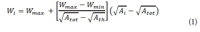
Where: A_th is the threshold area, A_totis the total area, and A is the area drained by the i^th cell.

These values are theappropriate initial values to create the model parameters. Hence, the values of the cell-specific parameters for all the cells were generated from the extracted thematic maps. After that, the implementation of the model additionally requires fixing the simulation periods, setting the simulation time-step and preparing the forcing files (variables), matching with spatial scale and time-step of the simulation. In defining the simulation periods, two independent periods of some suitable length must be available where the data are continuous and of good quality for the model evaluation. Accordingly, based on the availability of the data, the 2001-2010 data were used for calibration and that between 1986 and 2000 were used for validation for Gilgel Ghibe catchment. Similarly, the data from 1980-1994 were utilized for calibration and the 1995-2009 dataset was used for validation for Mhlanga catchment. The simulation time-step was chosen to be 24 h, which is highly suitable to simulate the main discharge variations for the study areas.

The respective daily rainfall and evapotranspiration data were used to create the 'rain-fields' and the 'ET' forcing files for the two catchments, respectively. Using these input files, we simulated the streamflow time series for both catchments.

 

RESULTS AND DISCUSSION

Overall results

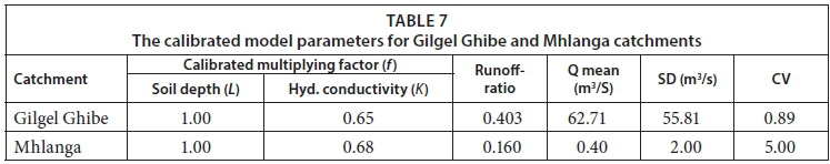
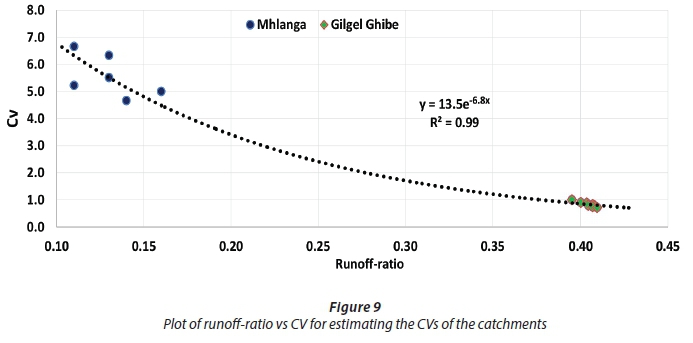
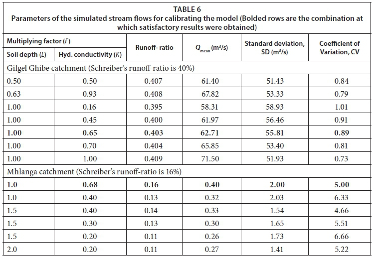
The two sensitive model parameters (L and K) were optimized as explained above. Table 7 shows the final optimum calibrated sensitive model parameters. Here, we identified that the parameter adjustment factors were essentially identical for both catchments, which suggests the generality of our results in that it would work for other catchments as well with the same parameter adjustment factors. This further supports the use of PyTOPKAPI model for ungauged catchments. Figure 9 indicates the plot of the CVs of the stream flows and the runoff-ratios for the two study catchments. We observed that the CV seems related to the runoff-ratio. A decreasing trend of CVs with increasing runoff-ratios is evident. As shown above, the Schreiber's runoff-ratios were 40% and 16% for the Gilgel Ghibe and Mhlanga catchments, respectively. Based on the above information and the plot in Fig. 9, the anticipated CV values were 0.89 and 5.0 for Gilgel Ghibe and Mhlanga catchments, respectively. The corresponding values of the optimum multiplying factors for the two sensitive parameters were then obtained as indicated (bolded rows) in Table 6.

Evaluation of the calibration

As a confirmation of the relevance of the calibration, the simulated stream flows of the catchments for the years of calibration are plotted in Figs 10a and b, respectively. The CV values obtained from the simulated results agreed with the estimated CV values for both of the catchments. It was also observed from scatter plots of cumulative rainfall volume and simulated runoff volume (Fig. 10 c and d) that there is, in general, good agreement between Schreiber's runoff-ratio and the simulated runoff-ratio for both catchments. To further realize the flow characteristics, comparison between observed and simulated stream flows was also done using flow-duration curves (Fig. 11). A flow-duration curve (FDC) is a cumulative frequency curve that shows the per cent of time during which the specified discharges are equalled or exceeded in a given period. It combines the flow characteristics of a stream throughout the range of discharges in one curve, without regard to the sequence of occurrence. It also provides a convenient means for studying the flow characteristics of streams and can be used to compare streams in different geomorphic settings. Subsequently, the overall comparisons in this perspective revealed that the model reasonably captured the stream flows, including extreme discharges and their timings. This further proves the capability of PyTOPKAPI model, together with the Schreiber's runoff-ratio, in modelling the stream flows from ungauged catchments.

Validation of the calibration

In order to validate the PyTOPKAPI model calibration using more reliable data, the model was applied to a different period of data, using the respective calibrated parameter values of the catchments and the hydro-meteorological dataset of the period between: (i) 1986 and 2000 for Gilgel Ghibe; and (ii) 1995 and 2009 for Mhlanga catchments. The simulated hydrographs are given in Fig. 12a and b, and scatter plots of cumulative volumes for the rainfall and simulated runoff are illustrated in Fig. 12 c and d. In this validation period, the simulated runoff-ratios and the CV values were observed to be in a good agreement with the target ones. In general, good simulation results were acquired for both catchments.

 

CONCLUSION AND RECOMMENDATIONS

Water resources are of great concern as they are closely linked to the well-being of humankind. Hydrological processes of a given region are often understood through studying river basins (Botai et al., 2015), for which sophisticated rainfall-runoff models are required. These rainfall-runoff models are powerful tools used in various water resource applications for simulating stream flows. However, most rivers of developing countries are poorly gauged/totally ungauged thereby resulting in limited data for calibration of models such as the PyTOPKAPI model. In this study, we examined the possibility of using the physically-based PyTOPKAPI model together with the Schreiber's runoff-ratio formula for applications to ungauged catchments. This method seems to be a new approach for model calibration in this context. The results suggest this can produce acceptable streamflow predictions. In summary, we concluded that the PyTOPKAPI model together with our simplified calibration approach, can be used to predict runoff responses from ungauged catchments for water resource applications and flood predictions in developing countries. We finally recommend further refinement of the approach by implementing it in other catchments.

 

REFERENCES

ARORA VK (2002) The use of the aridity index to assess climate change effect on annual runoff. J. Hydrol. 265 164-177. https://doi.org/10.1016/S0022-1694(02)00101-4        [ Links ]

ASANTE KO, ARTAN GA, PERVEZ S, BANDARAGODA C and VERDIN JP (2008) Technical Manual for the Geospatial Stream Flow Model (GeoSFM): United States Geological Survey Open-File Report 2007-1441. 65 pp. USGS, Reston, Virginia.         [ Links ]

BERHANU B, SELESHI Y, DEMISSE SS and MELESSE AM (2015) Flow regime classification and hydrological characterization:a case study of Ethiopian rivers. Water 2015 7 3149-3165. doi:3110.3390/w7063149.         [ Links ]

BLANEY HF and CRIDDLE WD (1962) Determining consumptive use and irrigation water requirements. USDA Technical Bulletin 1275, US Department of Agriculture, Beltsville. https://en.wikipedia.org/wiki/Blaney%E2%80%93Criddle_equation.         [ Links ]

BLÖSCHL G (2013) Runoff Prediction in Ungauged Basins: Synthesis Across Processes, Places and Scales. Cambridge University Press, New York. https://doi.org/10.1017/CBO9781139235761        [ Links ]

BOTAI CM, BOTAI JO, MUCHURU S and NGWANA I (2015) Hydrometeorological research in South Africa: A review. Water 2015 7 1580-1594. https://doi.org/10.3390/w7041580        [ Links ]

CAMPBELL GS (1985) Soil Physics with Basic: Transport Models for Soil Plant systems. Elsevier Science, New York.         [ Links ]

CHEN J, WU X, FINLAYSON BL, WEBBER M, WEI T, LI M and CHEN Z (2014) Variability and trend in the hydrology of the Yangtze River, China: Annual precipitation and runoff. J. Hydrol. 513 403-412. https://doi.org/10.1016/j.jhydrol.2014.03.044        [ Links ]

CIARAPICA L and TODINI E (2002) TOPKAPI: a model for the representation of the rainfall-runoff process at different scales. Hydrol. Process. 16 207-229. https://doi.org/10.1002/hyp.342        [ Links ]

COCCIA G, CINZIA MAZZETTI C, ORTIZ EA and TODINI E (2009) Application of the TOPKAPI Model within the DMIP 2 Project, University of Bologna, Bologna, Italy; ProGea Srl, Bologna, Italy; HidroGaia, Paterna (Valencia), Spain.         [ Links ]

DEMISSIE TA (2013) Climate change impact on stream flow and simulated sediment yield to Gilgel Gibe 1 hydropower reservoir and the effectiveness of Best Management Practices. Dr.Ing thesis, Rostock Univerity.         [ Links ]

DOOGE JCI (1992) Sensitivity of runoff to climate change: a Hortonian approach. Bull. Am. Meteorol. Soc. 73 (12) 2013-2024. https://doi.org/10.1175/1520-0477(1992)073<2013:SORTCC>2.0.CO;2        [ Links ]

DUAN R, FEDLER CB and BORRELLI J (2012) Comparison of methods to estimate saturated hydraulic conductivity in Texas soils with grass. J. Irrig. Drainage Eng. 138 (4). https://doi.org/10.1061/(ASCE)IR.1943-4774.0000407        [ Links ]

EthioVisit.com (2016) Major Ethiopia Rivers. URL: https://www.ethiovisit.com/major-rivers-of-ethiopia/34/ (Accessed 17 November 2016).         [ Links ]

FAO/IIASA/ISRIC/ISS-CAS/JRC (2012) Harmonized World Soil Database (version 1.1). FAO, Rome, Italy and IIASA, Laxenburg, Austria. URL: http://webarchive.iiasa.ac.at/Research/LUC/External-World-soil-database/HTML/HWSD_Data.html?sb=4 (Accessed 29 March 2016).         [ Links ]

FISCHER G, NACHTERGAELE F, PRIELER S, VAN VELTHUIZEN HT, VERELST L and WIBERG D (2008) Global Agro-ecological Zones Assessment for Agriculture (GAEZ 2008). IIASA, Laxenburg, Austria and FAO, Rome, Italy. URL: http://www.fao.org/soils-portal/soil-survey/soil-maps-and-databases/harmonized-world-soil-database-v12/en/ (Accessed 29 March 2016).         [ Links ]

FRAEDRICH K (2010) A parsimonious stochastic water reservoir: Schreiber's 1904 Equation Am. Meteorol. Soc. 11 575-578. https://doi.org/10.1175/2009JHM1179.1        [ Links ]

FRAEDRICH K and SIELMANN F (2011) An equation of state for land surface climates. Int. J. Bifurcation Chaos 21 (12) 3577-3587. https://doi.org/10.1142/S021812741103074X        [ Links ]

FRAEDRICH K, SIELMANN F, CAI D, ZHANG L and ZHU X (2015) Validation of an ideal rainfall-runoff chain in a GCM environment. Water Resour. Manage. 29 313-324. https://doi.org/10.1007/s11269-014-0703-2        [ Links ]

GLCC (2008) Global Land Cover Characterization. "United States Geological Survey (USGS)", Global Land Cover Characteristics Data Base version 1.2, http://edcdaac.usgs.gov/glcc/globdoc1_2.php,         [ Links ].

GONZÁLEZ-ZEAS D, GARROTE L, IGLESIAS A and SORDO- WARD A (2012) Improving runoff estimates from regional climate models: a performance analysis in Spain. Hydrol. Earth Syst. Sci. 16 (6) 1709-1723. https://doi.org/10.5194/hess-16-1709-2012        [ Links ]

JABRO JD (1992) Estimation of saturated hydraulic conductivity of soils from particle size distribution and bulk density data. Trans. ASABE 35 (2) 557-560. https://doi.org/10.13031/2013.28633        [ Links ]

JARVIS A, REUTER HI, NELSON A and GUEVARA E (2008) Hole-filled SRTM for the globe Version 4, Available from the CGIAR-CSI SRTM 90m Database. URL: http://srtm.csi.cgiar.org (Accessed 17 February 2016).         [ Links ]

JEON J-H, LIM K and ENGEL B (2014) Regional calibration of SCS-CN L-THIA Model: Application for ungauged basins. Water 6 (5) 1339-1359. https://doi.org/10.3390/w6051339        [ Links ]

KAMRUZZAMAN M, SHAHRIAR M and BEECHAM S (2014) Assessment of short term rainfall and stream flows in South Australia. Water 6 (11) 3528-3544. https://doi.org/10.3390/w6113528        [ Links ]

LIU Y, SANG Y-F, LI X, HU J and LIANG K (2017) Long-term streamflow forecasting based on relevance vector machine model. Water 2017 9 9. https://doi.org/10.3390/w9010009        [ Links ]

LIU Z-Y, TAN B-Q, TAO X and XIE Z-H (2008) Application of a distributed hydrologic model to flood forecasting in catchments of different conditions. J. Hydrol. Eng. 13 378-384. https://doi.org/10.1061/(ASCE)1084-0699(2008)13:5(378)        [ Links ]

LIU Z, MARTINA MLV and TODINI E (2005) Flood forecasting using fully distributed model: Application of TOPKAPI model to Upper Xixian catchment. Hydrol. Earth Syst. Sci. 9 (4) 347-364. https://doi.org/10.5194/hess-6-859-2002        [ Links ]

LIU Z and TODINI E (2002) Towards a comprehensive physically- based rainfall-runoff model. Hydrol. Earth Syst. Sci. 6 (5) 859-881.         [ Links ]

MIDDLETON BJ and BAILEY AK (2005) Water Resources of South Africa (WR 2005). WRC Report Number TT 381/08. Water Research Commission, Pretoria.         [ Links ]

MIDGLEY D, PITMAN W and MIDDLETON B (1994) The surface water resources of South Africa 1990. WRC Report Nos. 298/1.1/94 to 298/6.2/94. Water Research Commission, Pretoria.         [ Links ]

MINASNY B and MCBRATNEY AB (2000) Evaluation and development of hydraulic conductivity pedotransfer functions for Australian soil. Aust. J. Soil Res. 38 906-926. https://doi.org/10.1071/SR99110        [ Links ]

MUALEM Y (1976) A new model for predicting the hydraulic conductivity of unsaturated porous media. Water Resour. Res. 12 513-522. https://doi.org/10.1029/WR012i003p00513        [ Links ]

NEGASH F (2012) Managing water for inclusive and sustainable growth in Ethiopia: Key challenges and priorities. Addis Ababa, Ethiopia.         [ Links ]

PEGRAM G, SINCLAIR S, VISCHEL T and NXUMALO N (2010) Soil moisture from satellites: Daily maps over RSA for flash flood forecasting, drought monitoring, catchment management & agriculture. WRC Report No. 1683/1/10. Water Research Commission, Pretoria.         [ Links ]

RAWLS W, BRAKENSIEK D and SAXTON K (1982) Estimation of soil water properties. Trans. ASCE 25 (5) 1316-1320 and 1328.         [ Links ]

RAWLS WJ, BRAKENSIEK DL and MILLER N (1983) Agricultural management effects on soil water processes. I: Soil water retention and GreenAmpt parameters. Trans. ASCE 26 1747-1752.         [ Links ]

RIES III KG (2007) The national streamflow statistics program: A computer program for estimating streamflow statistics for ungaged sites: U.S. Geological Survey Techniques and Methods 4-A6, 37 pp.         [ Links ]

SAEIDIFARZAD B, NOURANI V, AALAMI M and CHAU K-W (2014) Multi-site calibration of linear reservoir based geomorphologic rainfall-runoff models. Water 6 (9) 2690-2716. https://doi.org/10.3390/w6092690        [ Links ]

SANBORN SC and BLEDSOE BP (2006) Predicting streamflow regime metrics for ungauged streamsin Colorado, Washington, and Oregon. J. Hydrol. 325 (1-4) 241-261. https://doi.org/10.1016/j.jhydrol.2005.10.018        [ Links ]

SAXTON KE and RAWLS WJ (2006) Soil water characteristic estimates by texture and organic matter for hydrologic solutions. Soil Sci. Soc. Am. J. 70 (5) 1569-1578. https://doi.org/10.2136/sssaj2005.0117        [ Links ]

SAXTON KE, RAWLS WJ, ROMBERGER JS and PAPENDICK RI (1986) Estimating generalized soil water characteristics from texture. Soil Sci. Soc. Am. J. 50 1031-1036. https://doi.org/10.2136/sssaj1986.03615995005000040039x        [ Links ]

SINCLAIR S and PEGRAM GGS (2012) PyTOPKAPI - an open-source implementation of the TOPKAPI hydrological model, 16^th SANCIAHS Symposium, 1-3 October 2012, Pretoria.         [ Links ]

SINCLAIR S and PEGRAM GGS (2013a) HYLARSMET: A hydrologically consistent land surface model for soil moisture and evapotranspiration modelling over Southern Africa using remote sensing and meteorological data. technical report. WRC Report No. 2024/1/13. Water Research Commission, Pretoria.         [ Links ]

SINCLAIR S and PEGRAM GGS (2013b) A sensitivity assessment of the TOPKAPI model with an added infiltration module. J. Hydrol. 479 100-112. https://doi.org/10.1016/j.jhydrol.2012.11.061        [ Links ]

SMETTEM KRJ, OLIVER YM, HENG LK, BRISTOW KL and FORD EJ (1999) Obtaining soil hydraulic properties for water balance and leaching models from survey data. 1. Water retention. Aust. J. Agric. Res. 50 (2) 283-289. https://doi.org/10.1071/A97074        [ Links ]

SOBIERAJ JA, ELSENBEER H and VERTESSY RA (2001) Pedotransfe functions for estimating saturated hydraulic conductivity: Implications for modeling storm flow generation. J. Hydrol. 251 202-220. https://doi.org/10.1016/S0022-1694(01)00469-3        [ Links ]

STOLTE J, FREIJER JI, BOUTEN W, DIRKSEN C, HALBERTSMA JM VAN DAM JC, VAN DEN BERG JA, VEERMAN GJ and WOSTEN JHM (1994) Comparison of six methods to determine unsaturated soil hydraulic conductivity. Soil Sci. Soc. Am. J. 58 1596-1603. https://doi.org/10.2136/sssaj1994.03615995005800060002x        [ Links ]

STRETCH D and ZIETSMAN I (2004) The hydrodynamics of Mhlanga & Mdloti Estuaries: Flows, residence times, water levels and mouth dynamics. URL: https://www.researchgate. net/publication/242278038_THE_HYDRODYNAMICS_OF_ MHLANGA_MDLOTI_ESTUARIES_FLOWS_RESIDENCE_ TIMES_WATER_LEVELS_MOUTH_DYNAMICS.         [ Links ]

THORNTHWAITE CW (1948) An approach toward a rational classification of climate. Geogr. Rev. 38 (1) 55-94. https://doi.org/10.2307/210739        [ Links ]

THORNTHWAITE CW and MATHER JR (1955) The water balance. Publ. Climatol. Lab. Climatol. Dresel Inst. Technol. 8 (1) 1-104.         [ Links ]

UNU-INWEH (2016) United Nations University- Institute for Water, Environment and Health. The WaterBase project. URL: http://www.waterbase.org (Accessed November 02, 2016).         [ Links ]

VIS, M, KNIGHT R, POOL S, WOLFE W and SEIBERT J (2015) Model calibration criteria for estimating ecological flow characteristics. Water 2015 7 2358-2381. https://doi.org/10.3390/w7052358        [ Links ]

VISCHEL T, PEGRAM G, SINCLAIR S and PARAK M (2008) Implementation of the TOPKAPI model in South Africa: Initial results from the Liebenbergsvlei catchment. Water SA 34 331-342.         [ Links ]

WU M-C and LIN G-F (2015) An hourly streamflow forecasting model coupled with an enforced learning strategy. Water 2015 7 5876-5895. https://doi.org/10.3390/w7115876        [ Links ]

ZHANG Y, ENGEL B, AHIABLAME L and LIU J (2015) Impacts of climate change on mean annual water balance for watersheds in Michigan, USA. Water 2015 7 3565-3578. https://doi.org/10.3390/w7073565        [ Links ]

ZHAO N, YU F, LI C, WANG H, LIU J and MU W (2014) Investigation of rainfall-runoff processes and soil moisture dynamics in grassland plots under simulated rainfall conditions. Water 6 (9) 2671-2689. https://doi.org/10.3390/w6092671        [ Links ]

ZIETSMAN I (2003) The hydrodynamics of temporary open estuaries with case studies of Mhlanga and Mdloti. MSc thesis, University of KwaZulu-Natal.         [ Links ]

 

 

Received 30 March 2017
Accepted in revised form 14 March 2018

 

 

* To whom all correspondence should be addressed. ffi +27-84-599-6507; +251-91-186-4647; e-mail: zeinuahmedrabb@yahoo.com