


Servicios Personalizados
Articulo
 Inglés (pdf)
 Articulo en XML
 Referencias del artículo
Indicadores

Links relacionados
-
 Citado por Google
 -
 Similares en Google
Compartir

 Permalink
Water SA
versión On-line ISSN 1816-7950
versión impresa ISSN 0378-4738
Water SA vol.44 no.2 Pretoria abr. 2018
http://dx.doi.org/10.4314/wsa.v44i2.01
ORIGINAL ARTICLES
3-D numerical modelling of groundwater flow for scenario-based analysis and management
Muhammad UsmanI, III, *; Rudolf LiedlII; Muhammad ArshadI; Christopher ConradIII
IDepartment of Irrigation & Drainage, University of Agriculture, Faisalabad, Pakistan
IIInstitute for Groundwater Management, Technical University Dresden, Germany
IIIDepartment of Remote Sensing, Institute of Geography and Geology, University of Würzburg, Germany
ABSTRACT
In recent years, extensive competition for groundwater use among different consumers has exploited major freshwater aquifers in Pakistan. There is an urgent need for appraisal of this precious resource followed by some mitigation strategies. This modelling study was conducted in the mixed cropping zone of the Punjab, Pakistan. Both remote sensing and secondary data were utilized to achieve objectives of this study. The data related to piezometric water levels, canal gauges, well logs, meteorological and lithological information were collected from Punjab Irrigation Department (PID), Water and Power Development Authority (WAPDA). Groundwater flow models for both steady and transient conditions were set-up using FEFLOW-3D. Water balance components and recharge were estimated using empirical relations and inverse modelling approaches. Both manual and automated approaches were utilized to calibrate the models. Moreover, sensitivity analysis was performed to see the response of model output against different model input parameters. Followed by calibration and validation, the model was run for different management scenarios, including lining of canal sections, minimization of field percolation, and change of groundwater abstraction. The study results show a drop in groundwater levels for almost all scenarios. The highest negative change was observed for the 4th scenario (i.e. 25% increase in groundwater pumping over a 10-year period), with a value of 3.73 m, by ignoring very wet summer and winter seasons. For normal weather conditions, the highest negative change was observed for the 4th scenario with a value of 2.91 m followed by 2.68 m for the 3 scenario (i.e. 50% reduction in canal seepage and field percolation over a 10-year period). For very wet summer and winter seasons, only one positive change was observed, for the 5th scenario (i.e. 25% decrease in groundwater pumping during 10 years period), with a value of 1.17 m. The changes for all other scenarios were negative. The mitigation strategy may include less groundwater pumping, by supporting cultivation of low delta crops and adjusting cropping patterns considering canal water supplies. It is further suggested to support current modelling results by incorporating more detailed information on cropping and by exploring the effect of climate change.
Keywords:numerical modelling, sensitivity analysis, FEFLOW, scenario analysis, Pakistan
INTRODUCTION
About 70% of global groundwater resources are consumed by agriculture (Döll, 2009). The share of groundwater used is about 750-800 km3, which is about one-sixth of the total freshwater use (Shah, 2000). Although the share of groundwater used for agriculture is lower than that of surface water globally, the advantages of groundwater use, like on-demand availability, accessibility, reliability, and high productivity, outweighs those of surface water use (Qureshi et al., 2009).
Groundwater use is inevitable for agriculture in Pakistan. About 40 to 50% of irrigation water needs in the country are fulfilled by exploiting groundwater (Usman et al., 2015; Kazmi et al., 2012). The share of groundwater used for meeting domestic and industrial requirements is about 10%, and this value is growing due to urbanization, industrialization and improved living standards. Currently, in the Punjab Province, about 90% of daily domestic demands are met by groundwater. The consequences of this use include lowering of groundwater levels in many parts of the country, along with secondary secondary salinization and pumping costs (Qureshi et al., 2009). According to Qureshi (2010), there are about 21 canals commands (irrigated areas receiving water from a particular canal) in Punjab and Sindh Provinces where the groundwater table depth has fallen by up to 300 cm over a period of 10 years (1993-2002).
The current study was conducted in the lower parts of the Lower Chenab Canal (LCC), Punjab, Pakistan. The region is considered important for the production of agricultural commodities but the sustainability of groundwater use is challenging due to water quantity and quality issues. Analysis of electrical conductivity (EC) shows that the majority of the area, including Bhagat and Sultanpur irrigation subdivisions, has saline groundwater in deeper aquifer depths, with a high concentration of salts. According to locally conducted groundwater sampling results, about 64.5% and 59.4% of the area of Bhagat irrigation subdivision encompasses unfit groundwater during the post- and pre-monsoon seasons. Similarly, about 90% of the total area of Sultanpur irrigation subdivision has groundwater quality that is marginal during both pre- and post-monsoon seasons. Due to this salinity problem, there is always competition for surface water use and groundwater abstraction is considered mandatory, which results in up-coning of saline water and consequently decreased agricultural productivity.
Considering the importance of groundwater use for agriculture, its proper distribution needs to be ensured, for meeting the future demands of food and fibre, which will increase in coming decades due to increases in population. This is only possible through proper understanding of the problem in order to devise workable strategies. Quantitative solution of the problem using 3-D numerical modelling is a potential means to conceptualize the groundwater resources and to make viable plans for its sustainability (Al-Zyoud et al., 2015). This particular study demonstrates the use of numerical modelling for describing the problem and exploring the effects of different management scenarios on groundwater fluctuations.
STUDY AREA
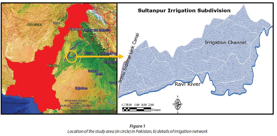
Location, climate and agriculture
Sultanpur irrigation subdivision was selected as a case study region in the LCC (Fig. 1). LCC off-takes from Khanki head-work on the river Chenab. The major crops cultivated include sugarcane, fodder and cotton in kharif and wheat during rabi cropping season. The two cropping seasons, rabi and kharif, usually prevail from November to April and from May to October, respectively.
Geological settings
The study area is a part of an abandoned floodplain, which is underlain by highly stratified unconsolidated alluvial material composed of sand of various grades interbedded with discontinuous lenses of silt, clay and nodules of kanker - a calcium carbonate of secondary origin deposited by present and ancestral tributaries of the Indus River. The bottom of the aquifer is formed by metamorphic and igneous rocks of Precambrian age (Sarwar and Eggers, 2006). The horizontal conductivity is generally an order greater than vertical (Usman et al., 2015). Khan (1978) has synthesized the results of pumping tests, lithological and mechanical analyses of the test boreholes, and reports that hydraulic conductivity varies from 24 to 264 m-day-1 and specific yield from 1 to 33% in different parts of LCC.
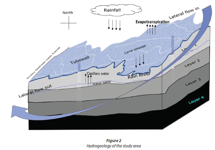
Hydrogeology/conceptual model
The conceptual model of the study area is shown in Fig. 2. The model area is bounded by a Trimu-Sidhnai link canal and the River Ravi on its western and southern sides. The northern and part of the eastern model boundaries are not connected with any water body and so interact with the modelling region through lateral groundwater inflow and outflow. The sections were identified using contour maps and lateral inflows/ outflows were estimated by Darcy's Law (Usman et al., 2015). Overall, the groundwater flow is parallel to this model boundary in a direction from north-east to south-west. The region is equipped with a wide irrigation network consisting of main canals, branch canals, major and minor distributaries. The irrigation water is supplied through the lower Chenab canal irrigation network. The transport of water through this irrigation network contributes a major recharge to groundwater at different stages of the irrigation system. The elevation of the region drops smoothly from north-east to south-west and causes regional groundwater flow along this elevation drop. As land use in the area is dominated by agriculture, groundwater pumping occurs along with canal water use. The major proportion of recharge takes place from monsoon rainfall and also from field percolation losses. The climate is regarded as semi-arid with high air temperatures which cause huge evapotranspiration losses.
Data acquisition and processing
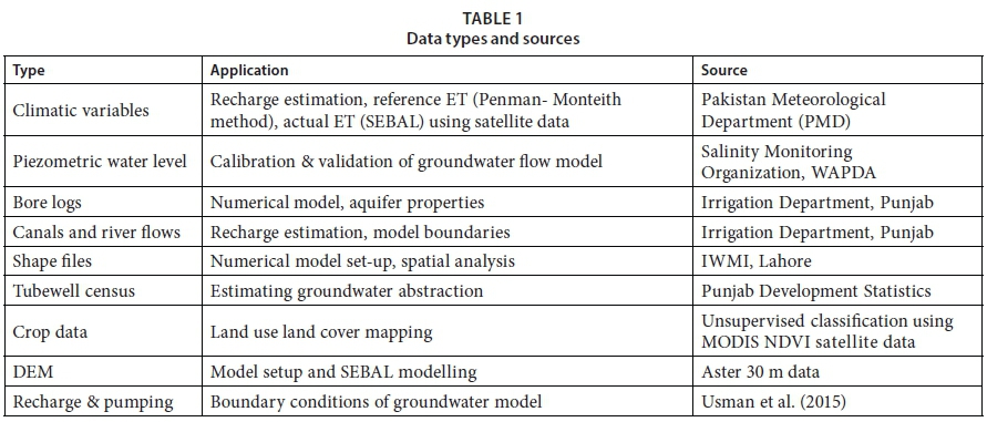
Table 1 summarizes different data types utilized for the current study and its acquisition from different sources.
Setting of numerical model and scenario-based simulations
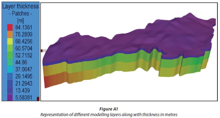
The triangular mesh algorithm (Shewchuk, 2005) was selected for finite element meshing owing to its fast speed and its capability to accommodate polygons, lines and points. The mesh quality was tested by Delaunay criteria for ensuring maximum model stability. Projection of 3-D unsaturated aquifer with saturation case was selected as the problem class. The aquifer was subdivided into 4 layers and 5 slices with the upper-most layer set as phreatic (i.e. unconfined). The thickness of different modelling layers was decided on the basis of the hydrogeological model and strata information from bore log data (Figure A1, Appendix). The total number of nodes per slice and elements per layer were 15 and 243, and 30 and 765, respectively. Both steady and transient models were prepared. The head results of the steady model were utilized as initial conditions for the transient model. Regionalization of both hydraulic conductivity and specific yield were performed using Akima interpolation algorithm (Akima, 1970) with linear interpolation type, with 5neighbours and zero over/ undershooting criteria. 'Constant' (i.e. no time step) was used for the steady model, whereas for the transient model, the Adams-Bashforth time stepping scheme was used. The Adams-Bashforth scheme is an automatic time-step control scheme which gives good convergence and stability to model runs. PARDISO - Parallel Direct Solver (Schenk and Gärtner, 2004) was chosen for solving the equation system.
Model boundary conditions
In FEFLOW, recharge is considered as a material property instead of a boundary condition, which is estimated by using a water balance approach and modelling techniques, as can be seen in Usman et al. (2015). The recharge is assigned as a time-variant material property to the transient model. Prescribed head boundary conditions were assigned along the Trimu Sidhnai link canal and river Ravi based on their historical water-level records (Sarwar and Eggers, 2006), and by working out the water levels in the course of the channel with DEM. The Dirichlet type, time-varying boundary conditions were applied instead of Cauchy-type boundary conditions. The Cauchy boundary condition requires channel bed conductance and its geometry data, which were inaccessible from any source. With the eastern and northern model sides, Neumann-type boundary conditions were employed, for which the inflow and outflow sections and flow to the model domain were identified using piezometric water levels and by application of Darcy's law. The detailed methodology can be seen in Usman et al. (2015). Nodal source/sink boundary condition was applied for groundwater pumping. The rates of pumping were estimated separately for all seasons employing a procedure described in Usman et al. (2015).
Model calibration, validation and sensitivity analysis
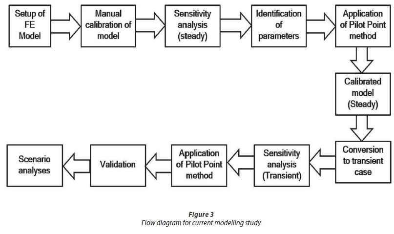
Figure 3 presents the flow diagram showing how calibration, validation and sensitivity analyses were conducted in the current study. The calibration of models was performed using both a manual approach and automated approach using PEST (Doherty, 2002). The pilot point technique (De Marsily et al., 1984) was used to define spatially variable parameters using kriging and each slice/layer of the model was treated as a single zone for performing the interpolation. The advanced Tikhonov regularization was implemented in PEST to encounter non-uniqueness of parameters. Tikhonov regularization is implemented as the number of estimation parameters was quite large (246 pilot points in total). The sensitivity analyses were performed manually for both steady and transient models.
Recharge components
Estimation of recharge at different segments of the irrigation system is necessary to set up different management scenarios. For this purpose, a water balance approach was utilized and input data for the water balance model were taken from remote sensing and secondary sources. Recharge was estimated individually from each irrigation system segment of LCC. The detailed methodology of recharge estimation for LCC irrigation subdivisions, including Sultanpur, can be seen in Usman et al. (2015).
Statistical analysis
Different statistical parameters were used to evaluate the model performance. These parameters include correlation coefficient (r), Nash Sutcliffe efficiency (NSE) and mean square error (MSE) as defined below:
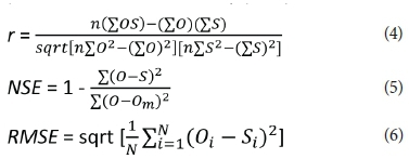
where O is measured (observed) data; Om is the mean of measured data; S is simulated data and S is the mean of the simulated data.
RESULTS AND DISCUSSION
Calibration and validation of models
A steady-state model was developed and its calibration was performed in the first phase. The groundwater heads for April 2005 (pre-monsoon period) were used for manual followed by automated calibration operation using PEST. The hydraulic conductivity was taken as the adjustment parameter to match the model heads with observed heads. The values of hydraulic conductivity were retrieved from the bore-logs and used as the pilot points for PEST calibration. Before employing automated calibration using PEST, manual calibration was performed to bring simulated heads close to observed heads. This practice helps one to understand the model system better and also facilitates reducing the automated calibration convergence time considerably, thus providing a check against model failure. About 34 manual model runs were performed before the automated run.
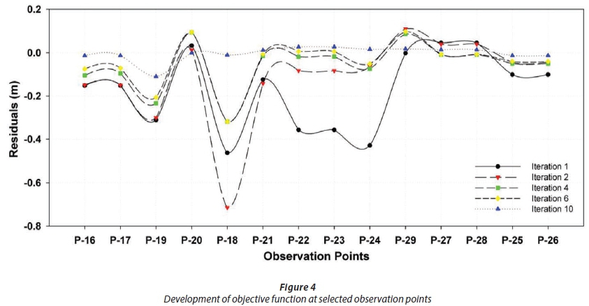
Following the steady-state model calibration, a transient model was developed using groundwater heads of the steady model as initial conditions. For the transient case, both hydraulic conductivity and specific yield were considered as calibration parameters. The initial and parameter bound values for these hydrological parameters were taken from the literature against different depth of well-logs collected during drilling. Again, before running the model in automated mode, manual calibration was performed to facilitate the automation process and smooth convergence of the modelling system. Again about 15 manual model runs were performed. The automated calibration parameters for PEST operation were adjusted where needed and the model was run in 'estimation' mode. The performance of the calibration development was observed in the form of an objective function as residuals for each iteration of PEST run were noted. The model converged in 10 iterations and at some locations the residuals were higher, but dropped near to zero in 10 iterations. The model run time in this case was about 7 h on an Intel Core i5-2410 M CPU at 2.30 GHz with 8.0 GB installed memory and 64-bit operating system. For automated calibration of the transient model, data from October 2005 to 2009 were utilized. Figure 4 shows the development of the objective function in different iterations, whereas Fig. 5 (a,b,c) shows the locations of observation points and scatter plots for simulated and observed heads for both steady and transient models after the calibration process.

Different statistical indicators showed very good results for both the steady and transient models. In the case of the steady model, the values of NSE and MSE were 0.98 and 0.23 m, while for the transient case these values were 0.97 and 0.28 m with correlation coefficients of 0.98 and 0.97, respectively. After performing the model calibration, validation of the model was performed and the results can be seen in Fig. 5(c). The validation of model results for the period 2009-2012 showed that the model performed reasonably well, as NSE and MSE were 0.96 and 0.31 m, while the correlation coefficient was 0.97. In general, the model performed very well for the upper model regions as most of the points were placed very near to the 1:1 line, but relatively more variation was observed in the middle and lower model regions. The setting of initial hydrologic parameters, and setting of boundary conditions for the river, could be the reason for this variation. Nevertheless, overall the results were reasonable, to be adopted for further model simulations.
Sensitivity analysis
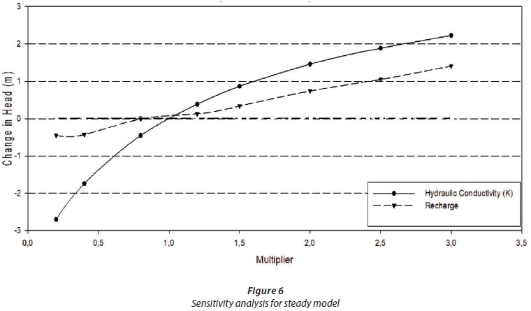
Variations in the hydrologic parameters and modelling simplifications are evaluated through sensitivity analysis of the modelling output. The sensitivity analysis was performed manually by uniformly multiplying hydraulic conductivity, specific yield and recharge by different multiplying factors. For each simulation, one parameter was changed at a time keeping other parameters unchanged. The multiplying factors used were 0.2, 0.4, 0.8, 1.2, 1.5, 2.0, 2.5, 3.0 throughout the interior nodes of the model and the model was rerun for each factor.
Figure 6 shows that higher sensitivity was observed for changes in hydraulic conductivity than recharge in the case of the steady model. The difference in head was higher for small multipliers up to 1.5, which became small for higher factor values. The sensitivity was less for smaller recharge factors, which became higher for greater factor values.
For the transient case (Fig. 7), sensitivity was observed to be relatively higher for hydraulic conductivity followed by specific yield and recharge. The sensitivity was found to be relatively higher for large multipliers for both recharge and specific yield. However, positive and negative changes in groundwater heads are observed for recharge and specific yield, respectively. The possible reason is availability of more water for the modelling domain from groundwater recharge and low storage due to higher values of specific yield.
Scenario analyses
To explore the future trends of groundwater behaviour under different management scenarios, simulations were run for a one-decade time period. Different weather conditions (i.e., precipitation) were considered for running the simulations, including normal weather (i.e., precipitation) conditions, very wet summer and winter conditions, and dry summer and winter conditions. The different weather conditions are worked out by calculating the average of 30 years of precipitation data, from 1970 to 2000, for a weather station located in Faisalabad, near the study area. Then the average values were compared to each season and year separately and three types of weather conditions identified, including normal weather conditions, weather conditions with higher rainfall and weather conditions with lower rainfall than average. Under each weather condition, five hypothetical water management scenarios were run, which included a 50% reduction in canal seepage in a 10-year period (1st), 50% reduction in field percolation in a 10-year period (2nd), 50% reduction in canal seepage and field percolation over 10 years (3rd), 25% increase in groundwater pumping over 10 years (4th), and 25% decrease in groundwater pumping over 10 years (5th). The baseline time considered for all the scenarios was 15 September, 2011 (i.e. Julian Day 40801).
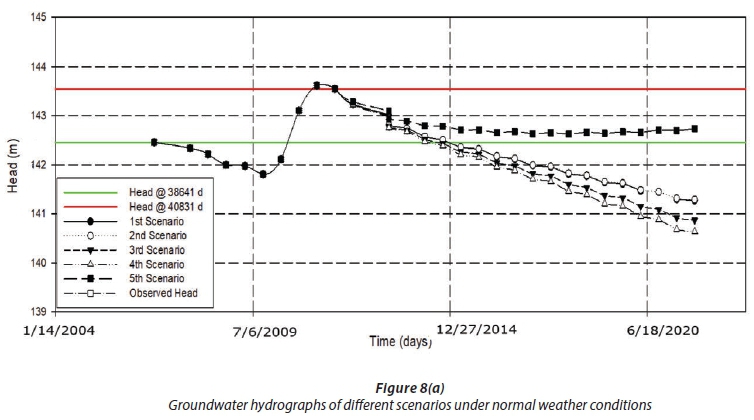
The groundwater levels were never stable during the calibration and validation periods with a decrease and increase in trends during the first and second halves of the simulation period, respectively. Figure 8(a) shows that under normal weather conditions, groundwater levels decreased steadily in all of the scenarios, except for the 5th scenario, where groundwater level first decreased but then remained stable for the rest of the simulation period. In this scenario, the groundwater level never dropped below the groundwater level at the start of the model run (i.e. Julian Day 38641).
In the second type of scenario run (Fig. 8b), ignoring very wet summer and winter weather conditions, groundwater drop was accelerated and a groundwater drop of about ~3.0 m was observed for all scenarios except the 5th scenario. However, under such weather conditions, the groundwater dropped below the level at the start of the model simulation run (i.e. Julian Day 38641).
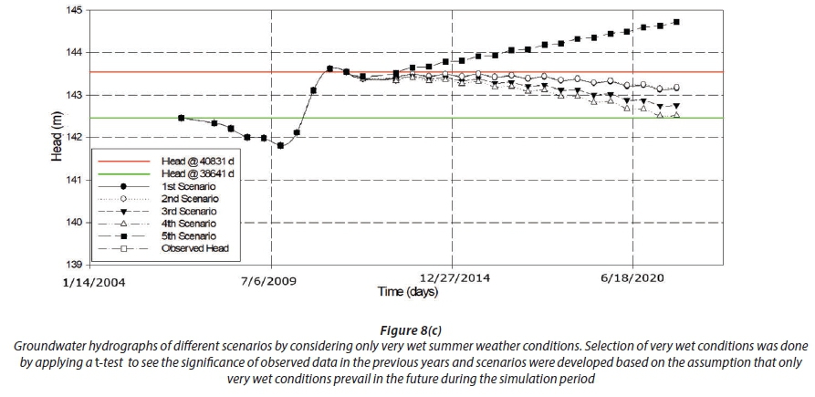
For scenario runs considering very wet summer weather conditions (Fig. 8c), the groundwater remained almost stable within a range of about ~ 1.0 m for all scenarios except the 5th scenario, where groundwater developed positively during the simulation period. In all types of weather conditions, the drop in groundwater level was greatest in the 4th scenario, which indicate that if groundwater pumping should increase without introducing any water management intervention then groundwater resources could be at risk of diminishing. In the present study, all of these scenarios were run separately; however, results indicate that groundwater drop could be minimized if different scenarios were run in combination, which encourages the implementation of different on-farm and water management practices in the region. The increase in groundwater levels during wet years further strengthens the possibility of sustainable water management in this area. The possible water management solutions may include replacing of high delta crops like rice and sugarcane with less water consumptive crops. Moreover, water allowance needs to be revisited and cropping patterns may be adjusted to minimize the gap between demand and supply of canal water
SUMMARY AND CONCLUSIONS
Sultanpur irrigation subdivision, located in the lower reaches of the Lower Chenab Canal (LCC) is an important region for agriculture. The productivity of crops and secondary salinization are major issues due to over-pumping of saline water from deeper aquifer depths. This situation demands a quantitative appraisal of groundwater resources in the region. The current modelling study was performed using FEFLOW 3-D numerical model and results show that groundwater levels drop under most of the different hypothetical scenarios including decreased canal seepage, decreased field percolation, decreased/increased pumping. However, the results are only based on separate runs of different scenarios but there is scope for groundwater development if different scenarios (i.e. interventions) are introduced parallel to each other along with some occasional wet summer and winter weather conditions. The current study results can be further updated and strengthened by including possible changes in cropping patterns and climate change in the area.
ACKNOWLEDGEMENTS
We are thankful to HEC-DAAD for providing funding to conduct this study. Special gratitude is extended to DHI-WASY for providing a free-of-charge FEFLOW license for the current study.
REFERENCES
AKIMA H (1970) A new method of interpolation and smooth curve fitting based on local procedures. J. Assoc. Comput. Mach. 17 (4) 589-602. https://doi.org/10.1145/321607.321609 [ Links ]
AL-ZYOUD S, RÜHAAK W, FOROOTAN E and SASS I (2015) Over exploitation of groundwater in the centre of Amman Zarqa Basin -Jordan: Evaluation of well data and GRACE satellite observations. Resources 4 (4) 819-830. https://doi.org/10.3390/resources4040819 [ Links ]
DE MARSILY G, LAVEDAN G, BOUCHER M and FASANINO G (1984) Interpretation of interference tests in a well field using geo-statistical techniques to fit the permeability distribution in a reservoir model. Geostat. Nat. Resour. Characterization 2 831-849. https://doi.org/10.1007/978-94-009-3701-7_16 [ Links ]
DHI-WASY (2012) Reference manual of FEFLOW - Finite element subsurface flow and transport simulation system. User manual/ Reference manual/White paper release 6.1. WASY Ltd, Berlin. [ Links ]
DÖLL P (2009) Vulnerability to the impact of climate change on renewable groundwater resources: a global-scale assessment. Environ. Res. Lett. 4 035006. https://doi.org/10.1088/1748-9326/4/3/035006 [ Links ]
DOHERTY J (2002) Model-independent parameter estimation. Watermark Numer. Comput. 279. [ Links ]
KAZMI SI, ERTSEN MW and ASI MR (2012) The impact of conjunctive use of canal and tube well water in Lagar irrigated area, Pakistan. Phys. Chem. Earth A/B/C 47-48 86-98. [ Links ]
KHAN MA (1978) Hydrological data, Rechna Doab: lithology, mechanical analysis and water quality data of test holes/test-wells, Vol I. Publication no. 25, Project Planning Organization (NZ), Pakistan Water and Power Development Authority (WAPDA), Lahore. [ Links ]
QURESHI AS, GILL MA and SARWAR A (2010) Sustainable groundwater management in Pakistan: Challenges and opportunities. Irrig. Drainage 59 (2) 107-116. https://doi.org/10.1002/ird.455 [ Links ]
QURESHI AS, MCCORNICK, PG, SARWAR A and SHARMA BR (2009) Challenges and prospects of sustainable groundwater management in the Indus Basin, Pakistan. Water Resour. Manage. 24 (8) 1551-1569. [ Links ]
SARWAR A and EGGERS H (2006) Development of a conjunctive use model to evaluate alternative management options for surface and groundwater resources. Hydrogeol. J. 14 (8) 1676-1687. https://doi.org/10.1007/s10040-006-0066-8 [ Links ]
SCHENK O and GÄRTNER K (2004) Solving unsymmetric sparse systems of linear equations with PARDISO. Future Generation Comput. Syst. 20 475-487. https://doi.org/10.1016/j.future.2003.07.011 [ Links ]
SCHEWCHUK JR (2005) Triangle: A two dimensional quality mesh generator and Delaunay triangulator. Version 1.6. Computer Science Division, University of California at Berkeley. [ Links ]
SHAH T (2000) Groundwater markets and agricultural development: A South Asian overview. In: Proceedings of regional groundwater management seminar. Pakistan Water Partnership, 9-11 October 2000. [ Links ]
USMAN M, LIEDL R and KAVOUSI A (2015) Estimation of distributed seasonal net recharge by modern satellite data in irrigated agricultural regions of Pakistan. Environ. Earth Sci.https://doi.org/10.1007/s12665-015-4139-7 [ Links ]
Received 20 July 2017
Accepted in revised form 12 March 2018
* To whom all correspondence should be addressed. e-mail: Muhammad.usman@uni-wuerzburg.de

