Hydraulic head and groundwater ¹¹¹Cd content interpolations using empirical Bayesian kriging (EBK) and geo-adaptive neuro-fuzzy inference system (geo-ANFIS)

 

 

Çağdaş Sağir^{I, II, *} ; Bedri Kurtuluş^II

^IUniversity of Poitiers, SFA-UMR 7285-IC2MP Institute of Chemistry of Poitiers: Materials and Natural Resources, Building B35, Albert Turpain 5^th Street, 86073 Poitiers, France
^IIMuğla Sıtkı Koçman University, Geological Engineering Department, Kötekli Campus, 48000 Menteşe, Muğla, Turkey

 

 

---

ABSTRACT

In this study, hydraulic head and ¹¹¹Cd interpolations based on the geo-adaptive neuro-fuzzy inference system (Geo-ANFIS) and empirical Bayesian kriging (EBK) were performed for the alluvium unit of Karabağlar Polje in Muğla, Turkey. Hydraulic head measurements and ¹¹¹Cd analyses were done for 42 water wells during a snapshot campaign in April 2013. The main objective of this study was to compare Geo-ANFIS and EBK to interpolate hydraulic head and ¹¹¹Cd content of groundwater. Both models were applied on the same case study: alluvium of Karabağlar Polje, which covers an area of 25 km² in Muğla basin, in the southwest of Turkey. The ANFIS method (called ANFIS_XY) uses two reduced centred pre-processed inputs, which are cartesian coordinates (XY). Geo-ANFIS is tested on a 100-random-data subset of 8 data among 42, with the remaining data used to train and validate the models. ANFIS_XY and EBK were then used to interpolate hydraulic head and heavy metal distribution, on a 50 m² grid covering the study area for ANFIS_XY, while a 100 m² grid was used for EBK. Both EBK- and ANFIS_XY-simulated hydraulic head and ¹¹¹Cd distributions exhibit realistic patterns, with RMSE < 9 m and RMSE < 8 µg/L, respectively. In conclusion, EBK can be considered as a better interpolation method than ANFIS_XY for both parameters.

Keywords: ANFIS, EBK, interpolation, hydraulic head, metal, ¹¹¹Cd, alluvium, Muğla

---

 

 

INTRODUCTION

Earth scientists (hydrologists, geologists, biogeochemists, etc.) are interested in understanding the behaviour of hydrosystems (Kurtulus et al., 2011; Flipo et al., 2012). Usually they first do experiments/observations in the field at specific locations and then try to distribute these observations/measurements both in space and time using modelling techniques that are based on abstractions. As part of the hydrosystem, aquifer systems play a decisive role in its behaviour and act as a reservoir. Metals and metalloids in these kinds of reservoirs might be assessed as pollutants according to their abundance. In the case of using polluted water stored in reservoirs for domestic, industrial or irrigational purposes, harmful side effects will most likely be encountered. Recent studies have shown that groundwater heavy metal contamination often cannot be detected, especially in cities (Huang et al., 2014). Pollutant sources could be artificial or natural. Industrial, agricultural and domestic waste might be the sources if they are continuous and the concentration of waste is high enough to pollute the water. Geological units which are in contact with groundwater could also be the source as they dissolve with water. The accumulable-stable characteristic and toxicity of heavy metals in groundwater make them very important pollutants worldwide (Okbah et al., 2014). In order to avoid negative effects and to ensure environmental sustainability, hydraulic head and pollutants must be examined together.

The state of an aquifer unit is characterized by the piezometric head or hydraulic head, measured as the water level in piezometers. The mapping of these point data is useful for many environmental applications, such as water resources management during high flow conditions. Estimations of hydraulic head distribution are frequently used to determine the capture zone of pumping wells. Hydraulic head maps are also important tools for earth dam monitoring (Rivest et al., 2008). They are also used to initialize distributed models, which are critical tools nowadays for managing water resources at the basin scale (Perkins and Sophocleous, 1999; Billen et al., 2007; Flipo et al., 2007, 2012, 2014). As reported in Flipo et al. (2012) many inverse methodologies in hydrogeology use hydraulic head maps as a pre-requisite (24 publications among 45). The mapping of hydraulic heads requires synchronous measurements, usually achieved with synchronous snapshot campaigns. Synchronous snapshot campaigns are feasible for relatively small aquifer units (~100 km²), such as the Orgeval basin (Kurtulus et al., 2011; Kurtulus and Flipo, 2012; Mouhri et al., 2013). The larger the aquifer unit, the longer the measurement campaign, which can last several years for regional aquifer systems (>100 000 km²) and therefore introduce uncertainties in the final mapping result (Tóth, 2002).

Understanding the temporal and spatial variations of the depth to groundwater is a prerequisite to achieve sustainable water use in a basin. Point measurements of water table levels are available, but what is needed are groundwater surfaces based on these measurements. Robust interpolation methods are needed to interpolate hydraulic head point measurements. Many such methods have been discussed in the literature (Kurtulus and Flipo, 2012).

On the one hand, a technique often used in earth sciences and especially in hydrogeology is kriging (Cressie, 1990; Rouhani and Myers, 1990; Weber and Englung, 1994; Zimmerman et al., 1999; Brochu and Marcotte, 2003; Theodossiou and Latinopoulos, 2006; Lyon et al., 2006; Ahmadi and Sedghamiz, 2007; Abedini et al., 2008; Renard and Jeannée, 2008; Ta'any et al., 2009; Buchanan and Triantafilis, 2009; Pardo-Igúzquiza et al., 2009; Sun et al., 2009; Canoğlu and Kurtuluş, 2017). A few authors have compared the efficiency of different interpolation techniques with kriging, cokriging, and kriging with external drift (Hoeksema et al., 1989; Boezio et al., 2006; Pardo-Igúzquiza and Chica-Olmo, 2007; Ahmadi and Sedghamiz, 2008; Bargaoui and Chebbi, 2008). Kriging using DEM information as an external drift seems to be the most efficient methodology for unconfined aquifer units (Desbarats et al., 2002; Rivest et al., 2008), which is in agreement with the high correlation between hydraulic head and soil surface in such systems (Tóth, 1962). In a recent study, Finzgar et al. (2014) revealed the applicability of empirical Bayesian kriging (EBK) to investigate the spatial distribution of soil metal contamination.

On the other hand, hydrologists have started to incorporate fuzzy logic and artificial neural network(ANN) concepts in their methodologies, with more than 500 papers published on this topic between 1999 and 2007 (Maier et al., 2010), and especially for rainfall-discharge transformation at the catchment scale (Johannet et al., 2007; Kurtulus and Razack, 2007; Lallahem and Mania, 2003; Minns and Hall, 2004). It has been noted that ANFIS (Takagi and M. Sugeno, 1985; Jang, 1993, 1995, 1996; Celikyilmaz and Turksen, 2009; Wang et al., 2009) exhibits better simulation performances than classical artificial neural networks (Nayak et al., 2004; El-Shafie et al., 2007; Firat, 2008; Pai et al., 2009; Wang et al., 2009; Maier et al., 2010). Moreover, ANFIS has already been successfully used to interpolate hydraulic head distribution (Lin and Chen, 2004; Kholghi and Hosseini, 2009; Flipo and Kurtulus, 2011; Kurtulus et al., 2011; Kurtulus and Flipo, 2012; Tapoglou et al., 2014).

A lack in the literature of comparison of ANFIS and EBK for interpolation of hydraulic head and a metal parameter provided the main motivation of this study. EBK and Geo-ANFIS were tested and compared with each other in order to determine their performance and practicality for hydraulic head and ¹¹¹Cd interpolation.

 

EXPERIMENTAL SITE AND DATA

The 25 km² study area was located in Karabağlar Polje, near the Muğla city centre, in the southwest of Turkey (Fig. 1). Elevation ranges from 606 m to 717 m. Average annual air temperature is 14.9°C, and mean annual precipitation is 1 222 mm. The study area is covered by a Quaternary alluvium unit with a thickness of 80-100 m (Fig. 1) (Atalay, 1980). Intensive agricultural activities and operations such as a drinking water treatment facility, lime quarry, sand and gravel quarry, industrial zone and swimming pool are situated in the area. Nevertheless, Kurtuluş and Sağır (2017) indicated that there is no groundwater pollution. The Jurassic Yılanlı formation, which is composed of dolomite, dolomitic limestone and limestone, underlies the Quaternary alluvium deposit (Kurttaş, 1997). Based on field observations, the Yılanlı formation has the most advanced karst features in the area and several dolines were also spotted where surface water flows and infiltrates the karst system during high-flow periods. A hydrogeological conceptual model of the study site and surroundings was created and a hydraulic connection between the area and Gökova springs (south of the study site) was revealed (Açıkel, 2012). The other geological unit, the Tertiary-Miocene aged Köprüçay formation, consists of conglomerate and limestone present to the south of the site.

The depths of the studied water wells ranged between 8 and 20 m and they penetrate only the Quaternary alluvium deposit. During a snapshot campaign in April 2013, hydraulic head measurement and water sampling were performed for 79 water wells. Heavy metal analyses for several elements were done. Based on the preliminary statistical characteristics (e.g. normal distribution) of elements and the absence of certain elements at certain wells, ¹¹¹Cd was chosen as the most suitable element to interpolate and for testing different interpolation methods; 38 data for ¹¹¹Cd were available for use. In order to get an approximately similar spatial distribution to the ¹¹¹Cd data, 42 data-points for hydraulic head were selected and analysed. Measured hydraulic head values were plotted against surface elevation with the objective of determining correlation (Fig. 2). High correlation between these parameters was expected for the alluvium aquifer, and for all of the measured 79 hydraulic head values, a highly correlation with ¹¹¹Cd was found (R² = 0.93). When the higher elevation values are excluded, there is poor correlation (R² = 0.24). According to these correlations, the studied aquifer is driven by the alluvium at the full scale. But in the areas at lower altitude where the dolines are situated, groundwater flow in the alluvium unit is affected by karst structures.

 

INTERPOLATION METHODS

Kriging

Geostatistics aims at providing quantitative descriptions of natural variables distribution in space and time (Matheron, 1978; Journel, 1986; Chilès and Delfiner, 1999). Initially developed to address ore reserve evaluation issues in mining (Isaaks and Srivastava, 1989), it is now commonly applied to environmental sciences such as hydrogeology, air, water and soil pollution (Goovaerts, 1997). Geostatistics is used to characterize the spatial structure of the variable of interest by means of a consistent probabilistic model. This spatial structure is characterized by the variogram, which describes how the variability between sampled concentrations increases with the distance between the samples. A variogram model is fitted to the experimental variogram for subsequent analysis. The interpolation technique, known as kriging, provides the 'best', unbiased, linear estimation of a regionalized variable at unsampled locations, where 'best' is defined in a least squares sense, as it aims to minimize the variance of estimation error (Chiles and Delfiner, 1999). As for the classical interpolations, the estimation by kriging of the concentration at any target cell is obtained by a linear combination of the available sample concentrations. The kriging differentiates only by the way of choosing the coefficients of this linear combination. Those coefficients are called kriging weights and depend on:

•The distances between the data and the target (like other classical interpolators)

•The distances between the original data themselves (data clustering)

•the spatial structure of the variable

The basic tool used for kriging is the semi-variogram γ (Eq. 1), defined as half the expectancy of deviation between values of samples separated by a distance h. In this case it produces the spatial variability of the variable Z(x):

where: E[V] defines the mathematical average of the coordinates of the vector V. If Z''(x) is the kriged value at location x, Z(x_i) is the known value at location x_1, λ_i is the weight associated with the data, μ is the Lagrange multiplier and y(x_ix_j) is the value of variogram corresponding to a vector with origin in x_i, and extremity in x_j, the general equation of Kriging estimator is:

 

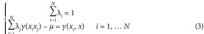
In order to achieve unbiased estimations in kriging and to minimize the variance of estimates the following set of equations should be solved simultaneously (Chauvet, 1999):

Empirical Bayesian kriging

Empirical Bayesian kriging (EBK) first appeared in the literature several years ago (Pilz and Spöck, 2007; Pilz et al., 2012). EBK is a geostatistical interpolation method that automates the difficult aspects of building a valid kriging model. Other kriging methods require one to manually adjust model parameters, but EBK automatically calculates these parameters through a process of sub-setting and simulations (Chiles and Delfiner, 1999). The EBK method can handle moderately non-stationary input data estimates and then uses many semi-variogram models rather than a single semi-variogram. EBK accounts for the error introduced by estimating the underlying semi-variogram through repeated simulations (Finzgar et al., 2014).

Geo-ANFIS

The adaptive neuro-fuzzy inference system (ANFIS) (Firat and Gungor, 2007; Jang, 1993, 1995, 1996; Pratihar, 2007; Takagi and Sugeno, 1985; Wang et al., 2009) is a modelling technique which assumes that input and output data are ill-defined with uncertainty that cannot be exactly assessed with probability theory based on a two-valued logic. It uses fuzzy set theory first proposed by Zadeh (1965). A fuzzy set is a set of elements with an imprecise (vague) boundary (Pratihar, 2007). A fuzzy set does not have a crisp boundary. That is, the transition from 'belonging to the set' to 'not belonging to the set' is gradual and is characterized by membership functions. A fuzzy set A(x) is then represented by a pair of two things - the first one is the constituent elements x and their associated membership values μ_A(x) that is their degree of belongingness:

where: X is the universal set consisting of all possible elements. The membership function μ_A ranges between 0 and 1. If the value of the membership function is restricted to either 0 and 1, the fuzzy set is then reduced to a classical crisp set with a known boundary. As stated by Jang (1995), the fuzziness does not come from the randomness of the constituent members of the sets, but from the uncertain and imprecise nature of the abstract thoughts and concepts.

In ANFIS the relationship between input and output is expressed in the form of If-Then rules. ANFIS used for the present work is based on the Sugeno fuzzy model (Takagi and M. Sugeno, 1985) which formalizes a systematic approach to generating fuzzy rules from an input-output dataset. A typical fuzzy rule in a Sugeno fuzzy model has the format: If x∊A and y∊B then:

where: A and B are fuzzy sets in the antecedent and f (x, y) is a crisp function in the consequent. Usually f is a polynomial function.

The architecture of the Geo-ANFIS is composed of 5 layers (Fig. 3). Each layer has a specific function. The first layer generates a membership grade of a linguistic label, which means that it defines the parameter of the membership function. For instance, consider a first-order Sugeno fuzzy inference system which contains 2 rules:

 

 

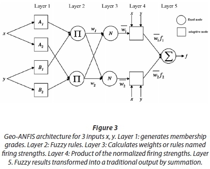
Rule 1: If X∊A₁ and Y∊B₁ then:

Rule 2: If X∊A₂ and Y∊B₂ then:

p₁, q₁, r₁, p₂, q₂, r₂ are defined in the first layer of the Geo-ANFIS (Fig. 3).

Each node i of Layer 2 calculates the firing strength w₁ of the i^th rule via multiplication:

Node i in Layer 3 calculates the ratio of the i^th rule's firing strength to the total amount of all firing strengths:

Node i in Layer 4 calculates the contribution (weight) of the i^th rule toward the overall output via multiplication:

Finally, Layer 5 is made on a single node that computes the overall output as the summation of the contribution from each rule:

ANFIS uses a hybrid learning algorithm that combines the back-propagation gradient descent and least squares method to create a fuzzy inference system whose membership functions are iteratively adjusted according to a given set of input and output data (Jang, 1993). For each iteration, the back-propagation method involves minimization of an objective function using the steepest gradient descent approach in which the network weights and biases are adjusted by moving a small step in the direction of a negative gradient. The iterations are repeated until a convergence criterion or a specified number of iterations is achieved. It has the advantage of allowing the extraction of fuzzy rules from numerical data and adaptively constructs a rule base.

Model implementation

Implementation of EBK

Exploratory data analysis, automatic variogram fitting and kriging were performed using ArcGis 10.2 software. The EBK method is based on 3 main steps: Firstly, a semi-variogram model is estimated from the observed data set. Secondly, a new value is simulated at each of the observed data locations by using the semi-variogram estimated in the previous step. Thirdly, a new semi-variogram model is estimated from the newly simulated data from the second step. By using Bayes' rule, a weight for this semi-variogram model is calculated which shows how likely it is that the observed data can be generated from the semi-variogram. The second and third steps are repeated. This process creates a spectrum of semi-variograms (Pilz and Spöck, 2007). New parameters are also needed for EBK, such as subset size which defines the number of points in each subset, overlap factor which specifies the degree of overlap between subsets and number of simulation which specifies the number of semi-variograms that will be simulated for each subset.

Implementation of Geo-ANFIS

The neuro-fuzzy model was developed using the ANFIS procedures of MATLAB (Demuth and Beale, 2000). In this study, a code is written in Matlab 2012b for ANFIS using appropriate functions to calculate the best performance of the methods.

Before using the model to interpolate unknown outputs (hydraulic head and ¹¹¹Cd), its actual predictive performance must be tested by comparing outputs estimated by calibrated models with known outputs. At each phase (training, validation and test), Geo-ANFIS performance is measured by the determination of the coefficient of goodness-of-fit (R²) and the root mean square error (RMSE).

where: E, Z^* and Z are previously defined.

Input data are XY coordinates for the ANFIS_XY. The data are pre-processed by elimination of unrealistic values to obtain a more stable dataset. Predictions of hydraulic head and ¹¹¹Cd are the Geo-ANFIS output.

The selection of appropriate input parameters is a complex task. At first step; numbers of training, validation and test data are decided by order: 60%, 20% and 20%. Assignment of data points to training, validation and test subsets is realized by random selection ability of ANFIS. Triangular (TriMF), Gaussian (GaussMF), Generalized bell (GbellMF), Spline-based (PiMF), Trapezoidal (TrapMF) and their different types of curves (named as 2, 3, 4 and 5) were used as membership functions in Geo-ANFIS. Random simulation number was decided as 100 which provides 100 different data assignments to training, validation and test subsets for each type of membership function curve. For ANFIS_XY simulations, the number of rules is set to 3 for each input.

 

SELECTION OF INTERPOLATION MODELS

EBK process

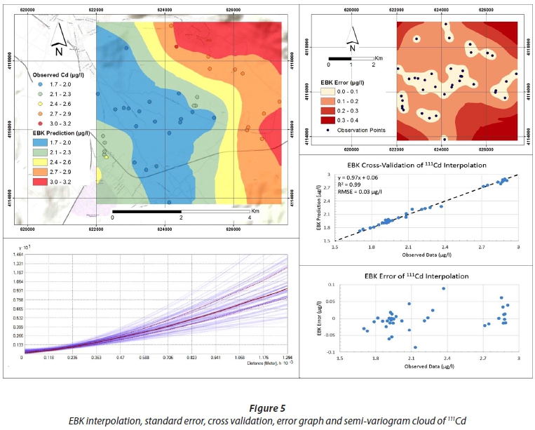
X-Y coordinates, hydraulic head and ¹¹¹Cd values were used as input to EBK. For the semivariogram cloud creation of hydraulic head; subset size, overlap factor, number of simulations, maximum neighbours, minimum neighbours and radius (m) are determined by order: 20, 2, 100, 15, 10 and 1 500. For the semivariogram cloud creation of ¹¹¹Cd; subset size, overlap factor, number of simulations, maximum neighbours, minimum neighbours and radius (m) are determined by order: 20, 2, 100, 15, 10 and 1500.

Geo-ANFIS model selection

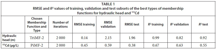
The Geo-ANFIS model selection is based on available data. Using these datasets at each phase (training, validation and test), the Geo-ANFIS performance is measured by the coefficient of goodness-of-fit (R²) and root mean square error (RMSE). ANFIS_XY is run up to 2 000 iterations with 100 random data simulations for 4 types of each membership function. 100 results for each type of membership function are analysed automatically to select the best ones. RMSE and R² values of training, validation and test subsets for the chosen types of membership functions for hydraulic head and ¹¹¹Cd are given in Table 1.

Testing of models

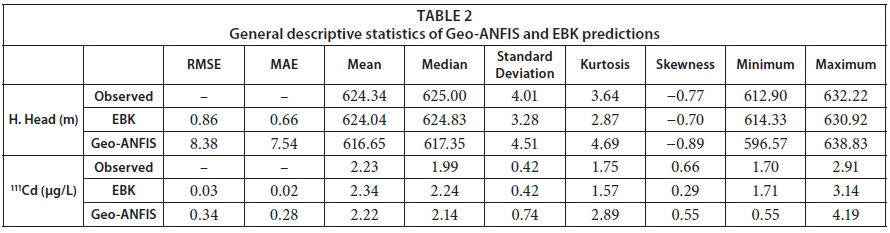
Geo-ANFIS and EBK predictions are assessed together based on RMSE, mean absolute error (MAE) and descriptive statistics given in Table 2. Performance of EBK is slightly better than Geo-ANFIS for both parameters interpolated. RMSE and MAE of EBK hydraulic head prediction values are 0.86 m and 0.66 m, whereas these values are 8.38 m and 7.54 m for Geo-ANFIS prediction. For EBK ¹¹¹Cd prediction, RMSE and MAE values are 0.03 µg/L and 0.02 µg/L. Besides the statistical values of hydraulic head prediction, map patterns were taken into consideration.

 

INTERPOLATIONS OF HYDRAULIC HEAD AND ¹¹¹CD

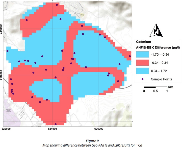
Hydraulic head and ¹¹¹Cd interpolation maps using EBK on a 100 m square grid are given in Fig. 4 and Fig. 5. Hydraulic head and ¹¹¹Cd distributions are calculated on a 50 m square grid for Geo-ANFIS and the maps are given in Fig. 6 and Fig. 7. Observed hydraulic head and ¹¹¹Cd values are directly used as input both in Geo-ANFIS and EBK. The EBK model produced less dispersed values for hydraulic head and ¹¹¹Cd with standard deviation of 3.28 m and 0.42 µg/L while Geo-ANFIS's are 4.51 m and 0.74 µg/L, respectively. RMSE between observed values and EBK prediction for hydraulic head and ¹¹¹Cd are 0.86 m and 0.03 µg/L while they are 8.38 m and 0.34 µg/L for Geo-ANFIS. EBK results are statistically the most consistent with the initial values. The Geo-ANFIS method prediction shows overestimation and underestimation for both parameters interpolated (Table 2). Also, the difference maps between EBK and Geo-ANFIS predictions for hydraulic head and ¹¹¹Cd are given in Fig. 8 and Fig. 9.

 

CONCLUSION

In this study, two interpolation methods were tested to estimate hydraulic head and ¹¹¹Cd distribution over the Karabağlar alluvium aquifer. Geo-ANFIS was used with 2 inputs as X-Y cartesian coordinates to interpolate hydraulic head and ¹¹¹Cd. Both hydraulic head and ¹¹¹Cd distribution results show that EBK performs considerably better than ANFIS_XY. Further, the prediction map generated by the Geo-ANFIS method doesn't represent smoothed results, as compared to all other interpolation methods.

For hydraulic head, Geo-ANFIS concluded with a 8.38 m RMSE value, which is significantly high when compared to the observed data range of 19.32 m. Also, for ¹¹¹Cd, Geo-ANFIS produced a 0.34 µg/L RMSE value while the observed data range is 1.21 µg/L. Geo-ANFIS performed better for ¹¹¹Cd than hydraulic head. In this regard, using X-Y cartesian coordinates and elevation for ANFIS (ANFIS_XYZ) may perform better, especially for interpolation of hydraulic head. However, the EBK RMSE value is 0.86 m for hydraulic head and 0.03 µg/L for ¹¹¹Cd. Hence, EBK gave better results for ¹¹¹Cd as well as hydraulic head.

In conclusion, EBK can be considered as better interpolation method than ANFIS_XY to interpolate hydraulic head and ¹¹¹Cd in groundwater. However, Geo-ANFIS proved its applicability as an alternative method to interpolate hydraulic head and metal concentration (¹¹¹Cd).

 

ACKNOWLEDGMENTS

We thank Sıtkı Koçman Foundation, French Embassy in Turkey, Muğla Sıtkı Koçman University-BAP (Project no: 12/141) and Tübitak & Eranetmed (No: 115Y843 & Name: "GRECPIMA") for their financial support. We would also like to thank Res. Asst. Göksu Uslular for his participation in the field.

 

REFERENCES

ABEDINI MJ, NASSERI M and ANSARI A (2008) Cluster-based ordinary kriging of piezometric head in West Texas/New Mexico - testing of hypothesis. J. Hydrol. 351 360-367. https://doi.org/10.1016/j.jhydrol.2007.12.030        [ Links ]

AÇIKEL Ş (2012) Gökova-Azmak (Muğla) karst kaynaklarının akım ve tuzlu su karışımı dinamiğinin kavramsal modellenmesi. PhD thesis, Hacettepe University.         [ Links ]

AHMADI SH and SEDGHAMIZ A (2007) Geostatistical analysis of spatial and temporal variations of groundwater level. Environ. Monit. Assess. 129 277-294. https://doi.org/10.1007/s10661-006-9361-z        [ Links ]

AHMADI SH and SEDGHAMIZ A (2008) Application and evaluation of kriging and cokriging methods on groundwater depth mapping. Environ. Monit. Assess. 138 357-368. https://doi.org/10.1007/s10661-007-9803-2        [ Links ]

ATALAY Z (1980) Muğla - Yatağan ve yakın dolayı karasal Neojen'inin stratigrafi araştırması. Turk. Jeol. Kurumu Bul. 23 93-99.         [ Links ]

BARGAOUI ZK and CHEBBI A (2008) Comparison of two kriging interpolation methods applied to spatiotemporal rainfall. J. Hydrol. 365 56-73. https://doi.org/10.1016/j.jhydrol.2008.11.025        [ Links ]

BILLEN G, GARNIER J, MOUCHEL JM and SILVESTRE M (2007) The Seine system: Introduction to a multidisciplinary approach of the functioning of a regional river system. Sci. Total Environ. 3751-12. https://doi.org/10.1016/j.scitotenv.2006.12.001        [ Links ]

BOEZIO M, COSTA J and KOPPE J (2006) Accounting for extensive secondary information to improve watertable mapping. Nat. Resour. Res. 15 33-48. https://doi.org/10.1007/s11053-006-9014-5        [ Links ]

BROCHU Y and MARCOTTE D (2003) A simple approach to account for radial flow and boundary conditions when kriging hydraulic head fields for confined aquifers. Math. Geol. 35 111-139. https://doi.org/10.1023/A:1023231404211        [ Links ]

BUCHANAN S and TRIANTAFILIS J (2009) Mapping water table depth using geophysical and environmental variables. Ground Water 47 80-96. https://doi.org/10.1111/j.1745-6584.2008.00490.x        [ Links ]

CANOĞLU MC and KURTULUŞ B (2017) Determination of the dam axis permeability for the design and the optimization of grout curtain: An example from Orhanlar Dam (Kütahya-Pazarlar). Period. Eng. Nat. Sci. 5 1. https://doi.org/10.21533/pen.v5i1.72        [ Links ]

CELIKYILMAZ A and TURKSEN IB (2009) Modeling Uncertainty with Fuzzy Logic. Springer, Berlin. 311 pp. https://doi.org/10.1007/978-3-540-89924-2        [ Links ]

CHAUVET P (1999) Aide-Mémoire de Géostatistique Linéaire. Ecole des mines de Paris, Paris. 312 pp.         [ Links ]

CHILES JP and DELFINER P (1999) Geostatistics: Modeling Spatial Uncertainty. John Wiley & Sons, Toronto. 726 pp.         [ Links ]

CRESSIE N (1990) The origins of kriging. Math. Geol. 22 239-252. https://doi.org/10.1007/BF00889887        [ Links ]

DEMUTH H and BEALE M (2000) Neural Networks Toolbox User Guide. Mathworks Inc. 840 pp.         [ Links ]

DESBARATS AJ, LOGAN CE, HINTON MJ and SHARPE DR (2002) On the kriging of water table elevations using collateral information from a digital elevation model. J. Hydrol. 255 25-38. https://doi.org/10.1016/S0022-1694(01)00504-2        [ Links ]

EL-SHAFIE A, TAHA MR and NOURELDIN A (2007) A neuro-fuzzy model for inflow forecasting of the Nile river at Aswan high dam. Water Resour. Manag. 21 533-556. https://doi.org/10.1007/s11269-006-9027-1        [ Links ]

FINZGAR N, JEZ E, VOGLA D and LESTAN D (2014) Spatial distribution of metal contamination before and after remediation in the Meza Valley, Slovenia. Geoderma 217 135-143. https://doi.org/10.1016/j.geoderma.2013.11.011        [ Links ]

FIRAT M (2008) Comparison of artificial intelligence techniques for river flow forecasting. Hydrol. Earth Syst. Sci. 12 123-138. https://doi.org/10.5194/hess-12-123-2008        [ Links ]

FIRAT M and GUNGOR M (2007) River flow estimation using adaptive neuro fuzzy inference system. Math. Comput. Simulat. 75 87-96. https://doi.org/10.1016/j.matcom.2006.09.003        [ Links ]

FLIPO N, JEANNÉE N, POULIN M, EVEN S and LEDOUX E (2007) Assessment of nitrate pollution in the Grand Morin aquifers (France): combined use of geostatistics and physically-based modeling. Environ. Pollut. 146 241-256. https://doi.org/10.1016/j.envpol.2006.03.056        [ Links ]

FLIPO N and KURTULUS B (2011) Geo-ANFIS: Application to piezometric head interpolation in unconfined aquifer unit. In: Proceedings of FUZZYSS'11The Second International Fuzzy Systems Symposium, 17-18 November 2011, Ankara.         [ Links ]

FLIPO N, MONTEIL C, POULIN M, FOUQUET C and KRIMISSA M (2012) Hybrid fitting of a hydrosystem model: long term insight into the Beauce aquifer functioning (France). Water Resour. Res. 48 W05509. https://doi.org/10.1029/2011wr011092        [ Links ]

FLIPO N, MOURHI A, LABARTHE B, BIANCAMARIA S, RIVIÈRE A and WEILL P (2014) Continental hydrosystem modelling: the concept of nested stream-aquifer interfaces. Hydrol. Earth Syst. Sci. 18 (8) 3121-3149. https://doi.org/10.5194/hess-18-3121-2014        [ Links ]

GOOVAERTS P (1997) Geostatistics for Natural Resources Evaluation. Oxford University Press, New York. 496 pp.         [ Links ]

HOEKSEMA RJ, CLAPP RB, THOMAS AL, HUNLEY AE, FARROW ND and DEARSTONE KC (1989) Cokriging model for estimation of water table estimation. Water Resour. Res. 25 429-438. https://doi.org/10.1029/WR025i003p00429        [ Links ]

HUANG GX, CHEN ZY and SUN JC (2014) Water quality assessment and hydrochemical characteristics of groundwater on the aspect of metals in an old town, Foshan, south China. J. Earth Syst. Sci. 123 91-100. https://doi.org/10.1007/s12040-013-0370-3        [ Links ]

ISAAKS E and SRIVASTAVA R (1989) An Introduction to Applied Geostatistics. Oxford University Press, New York. 580 pp.         [ Links ]

JANG JSR (1993) ANFIS adaptive-network-based fuzzy inference systems. IEEE Trans. Syst. Man Cybern. Syst. 23 665-685. https://doi.org/10.1109/21.256541        [ Links ]

JANG JSR (1995) Neuro-fuzzy modeling and control. In: Proc. IEEE 83 (3) 378-406. March 1995. https://doi.org/10.1109/5.364486        [ Links ]

JANG JSR (1996) Input selection for anfis learning. In: Proc. 5^th IEEE International Conference on Fuzzy Systems (Vol. 2 1493-1499) 11 September 1996. https://doi.org/10.1109/fuzzy.1996.552396        [ Links ]

JOHANNET A, AYRAL P and VAYSSADE B (2007) Modelling non-measurable processes by neural networks: Forecasting underground flow case study of the Ceze basin (Gard - France). In: Elleithy K (ed.) Advances and Innovation in Systems, Computing Sciences and Software Engineering. Springer, Dordrecht. https://doi.org/10.1007/978-1-4020-6264-3_10        [ Links ]

JOURNEL AG (1986) Geostatistics: Models and tools for the earth sciences. Math. Geol. 18 119-140. https://doi.org/10.1007/bf00897658        [ Links ]

KHOLGHI M and HOSSEINI SM (2009) Comparison of groundwater level estimation using neuro-fuzzy and ordinary kriging. Environ. Model. Assess. 14 729-737. https://doi.org/10.1007/s10666-008-9174-2        [ Links ]

KURTTAŞ T (1997) Gökova (Muğla) karst kaynaklarının çevresel izotop incelemesi. PhD thesis, Hacettepe University.         [ Links ]

KURTULUS B and FLIPO N (2012) Hydraulic head interpolation using anfis - Model selection and sensitivity analysis. Comput. Geosci. 38 43-51. https://doi.org/10.1016/j.cageo.2011.04.019        [ Links ]

KURTULUS B, FLIPO N, GOBLET P, VILAIN G, TOURNEBIZE J and TALLEC G (2011) Hydraulic head interpolation in an aquifer unit using ANFIS and ordinary kriging. In: Madani K, Duarado AC, Rosa A and Filipe J (eds) Computational Intelligence. Springer, Berlin. https://doi.org/10.1007/978-3-642-20206-3_18        [ Links ]

KURTULUS B and RAZACK M (2007) Evaluation of the ability of an artificial neural network model to simulate the input-output responses of a large karstic aquifer: The La Rochefoucauld (Charente, France). Hydrogeol. J. 15 (2) 241-254. https://doi.org/10.1007/s10040-006-0077-5        [ Links ]

KURTULUŞ B and SAĞIR Ç (2017) Karabağlar polyesinde yeraltı suyu metal-metaloit içeriğinin jeoistatistiksel yöntemlerle değerlendirilmesi (Muğla, Türkiye) Bull. Min. Res. Exp. 154 135-140.         [ Links ]

LALLAHEM S and MANIA J (2003) A nonlinear rainfall-runoff model using neural network technique: example in fractured porous media. Math. Comput. Model. 37 (9) 1047-1061. https://doi.org/10.1016/S0895-7177(03)00117-1        [ Links ]

LIN GF and CHEN LH (2004) A spatial interpolation method based on radial basis function networks incorporating a semivariogram model. J. Hydrol. 288 288-298. https://doi.org/10.1016/j.jhydrol.2003.10.008        [ Links ]

LYON SW, SEIBERT J, LEMBO AJ, WALTER MT and STEENHUIS TS (2006) Geostatistical investigation into the temporal evolution of spatial structure in a shallow water table. Hydrol. Earth Syst. Sci. 10 113-125. https://doi.org/10.5194/hess-10-113-2006        [ Links ]

MAIER HR, JAIN A, DANDY GC and SUDHEER KP (2010) Methods used for the development of neural networks for the prediction of water resource variables in river systems: Current status and future directions. Environ. Modell. Softw. 25 891-909. https://doi.org/10.1016/j.envsoft.2010.02.003        [ Links ]

MATHERON G (1978) Estimer et choisir. In: Les Cahiers du Centre de Morphologie Mathématique de Fontainebleau Fasicule 7, Ecole Nationale Supérieure des Mines de Paris, Paris.         [ Links ]

MINNS A and HALL M (2004) Rainfall-runoff modelling. In: Abrahart RJ, Kneale PE and See LM (eds) Neural Networks for Hydrological Modeling. A.A. Balkema Publishers, Leiden. https://doi.org/10.1201/9780203024119.ch9        [ Links ]

MOUHRI A, FLIPO N, REJIBA F, FOUQUET CD, BODET L, GOBLET P, KURTULUS B, ANSART P, TALLEC G, DURAND V and co-authors (2013) Designing a multi-scale sampling system of stream-aquifer interfaces in a sedimentary basin. J. Hydrol. 504 194-206. https://doi.org/10.1016/j.jhydrol.2013.09.036        [ Links ]

NAYAK PC, SUDHEER KP, RAGAN DM and RAMASASTRI KS (2004) A neuro-fuzzy computing technique for modeling hydrological time series. J. Hydrol. 291 52-66. https://doi.org/10.1016/j.jhydrol.2003.12.010        [ Links ]

OKBAH MA, NASR SM, SOLIMAN NF and KHAIRY MA (2014) Distribution and Contamination Status of Trace Metals in the Mediterranean Coastal Sediments, Egypt. Soil Sediment Contam. 23 656-676. https://doi.org/10.1080/15320383.2014.851644        [ Links ]

PAI TY, WAN TJ, HSU ST, CHANG TC, TSAI YP, LIN CY, HU HC and YU LF (2009) Using fuzzy inference system to improve neural network for predicting hospital wastewater treatment plant effluent. Comput. Chem. Eng. 33 1272-1278. https://doi.org/10.1016/j.compchemeng.2009.02.004        [ Links ]

PARDO-IGÚZQUIZA E and CHICA-OLMO M (2007) KRIGRADI: A cokriging program for estimating the gradient of spatial variables from sparse data. Comput. Geosci. 33 497-512. https://doi.org/10.1016/j.cageo.2006.08.004        [ Links ]

PARDO-IGÚZQUIZA E, CHICA-OLMO M, GARCIA-SOLDADO MJ and LUQUE-ESPINAR JA (2009) Using semivariogram parameter uncertainty in hydrogeological applications. Ground Water 47 25-34. https://doi.org/10.1111/j.1745-6584.2008.00494.x        [ Links ]

PERKINS SP and SOPHOCLEOUS M (1999) Development of a comprehensive watershed model applied to study stream yield under drought conditions. Ground Water 37 418-426. https://doi.org/10.1111/j.1745-6584.1999.tb01121.x        [ Links ]

PILZ J, KAZIANKA H and SPÖCK G (2012) Some advances in Bayesian spatial prediction and sampling design. Spat. Stat. 1 65-81. https://doi.org/10.1016/j.spasta.2012.03.003        [ Links ]

PILZ J and SPÖCK G (2007) Why do we need and how should we implement Bayesian Kriging methods. Stoch. Env. Res. Risk A. 22 (5) 621-632. https://doi.org/10.1007/s00477-007-0165-7        [ Links ]

PRATIHAR DK (2007) Soft Computing. Alpha Science International Ltd, Oxford. 246 pp.         [ Links ]

RENARD F and JEANNEE N (2008). Estimating transmissivity fields and their influence on flow and transport: The case of Champagne mounts. Water Resour. Res. 44 1-12. https://doi.org/10.1029/2008WR007033        [ Links ]

RIVEST M, MARCOTTE D and PASQUIER P (2008) Hydraulic head field estimation using kriging with an external drift: A way to consider conceptual model information. J. Hydrol. 361 349-361. https://doi.org/10.1016/j.jhydrol.2008.08.006        [ Links ]

ROUHANI S and MYERS DE (1990) Problems in space-time kriging of geohydrological data. Math. Geol. 22 611-623. https://doi.org/10.1007/BF00890508        [ Links ]

SUN Y, KANG S, LI F and ZHANG L (2009) Comparison of interpolation methods for depth to groundwater and its temporal and spatial variations in the Minqin oasis of northwest China. Environ. Modell. Softw. 24 1163-1170. https://doi.org/10.1016/j.envsoft.2009.03.009        [ Links ]

TA'ANY RA, TAHBOUB AB and SAFFARINI GA (2009) Geostatistical analysis of spatiotemporal variability of groundwater level fluctuations in Amman-Zarqa basin, Jordan: a case study. Environ. Geol. 57 525-535. https://doi.org/10.1007/s00254-008-1322-0        [ Links ]

TAKAGI T and SUGENO M (1985) Fuzzy identification of systems and its applications to modeling and control. IEEE Trans. Syst. Man. Cybern. Syst. 15 116-132. https://doi.org/10.1109/TSMC.1985.6313399        [ Links ]

TAPOGLOU E, KARATZAS GP, TRICHAKIS IC and VAROUCHAKIS EA (2014) A spatio-temporal hybrid neural network Kriging model for groundwater level simulation. J. Hydrol. 519 3193-3203. https://doi.org/10.1016/j.jhydrol.2014.10.040        [ Links ]

THEODOSSIOU N and LATINOPOULOS P (2006) Evaluation and optimisation of groundwater observation networks using the Kriging methodology. Environ. Modell. Softw. 21 991-1000. https://doi.org/10.1016/j.envsoft.2005.05.001        [ Links ]

TÓTH J (1962) a theory of groundwater motion in small drainage basins in central Alberta, Canada. J. Geophys. Res. 67 4375-4387. https://doi.org/10.1029/JZ067i011p04375        [ Links ]

TÓTH J (2002) József Tóth: An autobiographical sketch. Ground Water 40 320-324.         [ Links ]

WANG WC, CHAU KW, CHENG CT and QIU L (2009) A comparison of performance of several artificial intelligence methods for forecasting monthly discharge time series. J. Hydrol. 374 294-306. https://doi.org/10.1016/j.jhydrol.2009.06.019        [ Links ]

WEBER DD and ENGLUNG EJ (1994) Evaluation and comparison of spatial interpolators II. Math. Geol. 26 589-604. https://doi.org/10.1007/BF02089243        [ Links ]

ZADEH LA (1965) Fuzzy sets. Inform. Control. 8 338-353. https://doi.org/10.1016/S0019-9958(65)90241-X        [ Links ]

ZIMMERMAN D, PAVLIK C, RUGGLES A and ARMSTRONG MP (1999) An experimental comparison of ordinary and universal kriging and inverse distance weighting. Math. Geol. 31 375-390.         [ Links ]

 

 

Received 10 May 2016
Accepted in revised form 4 July 2017

 

 

* To whom all correspondence should be addressed: Tel: +90 532 057 18 77; e-mail: cagdassagir@gmail.com