


Servicios Personalizados
Articulo
 Inglés (pdf)
 Articulo en XML
 Referencias del artículo
Indicadores

Links relacionados
-
 Citado por Google
 -
 Similares en Google
Compartir

 Permalink
Water SA
versión On-line ISSN 1816-7950
versión impresa ISSN 0378-4738
Water SA vol.43 no.2 Pretoria abr. 2017
http://dx.doi.org/10.4314/wsa.v43i2.11
Modelling the effect of land use change on hydrological model parameters via linearized calibration method in the upstream of Huaihe River Basin, China
Wei SiI, II, III, *; Weimin BaoIII; Simin QuIII; Minmin ZhouIII; Peng ShiI, III; Xiaoqiang YangIV
IState Key Laboratory of Hydrology-Water Resources and Hydraulic Engineering, Hohai University, Nanjing, China 210098
IIBusiness School of Hohai University, Nanjing, 210098, China
IIICollege of Water Resources and Hydrology, Hohai University, Nanjing, 210098, China
IVHelmholtz Centre for Environmental Research -UFZ, Brückstrasse3a, Magdeburg,39114, Germany
ABSTRACT
Conceptual rainfall-runoff models have become a basic tool for evaluating effects of land use/cover changes on the hydrologic processes in small-scale as well as large watersheds. The runoff-producing mechanism is influenced by land use/cover changes. In this study, we analysed the effect of land use change on hydrological model parameters by calibrating the model parameters of different time periods with different land use via a linearized calibration method. The parameter calibration of a conceptual model usually involves the construction of objective function and optimization methods for good performance of observed data. However, the objective function of the minimum-sum-squared error will introduce an unrelated optimum solution for the parameter calibration problem of a conceptual model, which belongs to a highly complex nonlinear system. Thus, a linearized parameter calibration method, which searches for the optimal value on a parameter surface, is presented, based on the analysis of the problems of the objective function of the minimum-sum-squared error. Firstly, an ideal model is shown that illustrates the efficiency and applicability of this method. Secondly, the novel method is demonstrated for solving the Xinanjiang daily model parameter calibration. Finally, 50 years of data are divided into 4 different periods for parameter comparison, through which the effects of land use/cover changes on runoff in Dapoling watershed are evaluated. The results show that the linearized parameter calibration method is convergent, reasonable and effective. For example, the model parameter of evapotranspiration coefficient KC varied considerably, from 0.658 to 0.922, in response to land use/cover change within the watershed.
Keywords: land use/cover change; parameter calibration; linearized; upper Huaihe River Basin
INTRODUCTION
Conceptual rainfall-runoff models have been widely used for quantification of the effect of land use and land cover change on runoff dynamics (Burns et al., 2005; Jiang et al., 2004, Wan and Yang, 2004; Wang et al., 2007; Yuan and Shi, 2001; Zhang et al., 2004). The runoff-producing mechanism and hydrological response will be influenced by land use/cover changes, and this influence can be reflected by the calibrated parameter values of different time periods (Tao et al., 2015; Zhang et al., 2016; Zhong-Bo et al., 2014). A good model performance is critical to evaluate the effect of land use/cover change on hydrological processes. The major difficulty is that these models generally have a large number of parameters that cannot be obtained directly from field measurements; hence, model calibration is needed (Chen and Chau, 2006; Wang et al., 2009; Wu et al., 2009). The process of model calibration is normally done either manually or by using computer-based, automated procedures. Because of the time-consuming nature of manual calibration and the difficulty in explicitly assessing the confidence of model simulations, automation of the calibration process has been explored (Gupta et al., 1998; Gupta et al., 1998; Hendrickson et al., 1988; Johnston and Pilgrim, 1976; Yapo et al., 1996). Research into automated optimization methods has led to the development of stochastic global optimization searching methods based on extending the search area or increasing the number of initial optima (Cheng et al., 2002; Cheng et al., 2008; Duan et al., 1992; Franchini, 1996; Franchini and Galeati, 1997; Ritzel et al., 1994; Savic et al., 1999; Vasquez et al., 2000; Wang, 1991).
Rainfall-runoff model calibration is a highly complex nonlinear problem (Chau, 2007; Cheng et al., 2005; Muttil and Chau, 2006; Taormina et al., 2012). A successful calibration depends not only on effective optimization methods, but also on the calibration objective. Minimum-sum-squared error (MSSE) has been widely used as an objective function (Bárdossy and Singh, 2008; Bao, 1991; Bao et al., 2004; Rusli et al., 2015; Zádor et al., 2006). This objective function has been shown to work well in linear parameter calibration, which has been proved to attain the unique optimal value. However, it will introduce an unrelated local optimal into parameter calibration of the nonlinear function.
Therefore, a more convenient and efficient method for parameter estimation of hydrological models is to study the hydrological model parameters, model structure and hydrological simulation. In this paper, a methodology for system decomposition and degeneration of dimensionality has been developed in the calibration of the Xinanjiang model. The objective of degeneration is to reduce the number of parameters being optimized simultaneously to at least 3 or fewer. An ideal model was used to verify the efficiency and applicability of this method. Finally, this linearized calibration method was applied for Xinanjiang model parameter calibration to evaluate the effect of land use/cover change on the runoff of the upper Huaihe River Basin. We only compare the best calibrated parameters of different periods to assess the influence of land use change on runoff generation via this fast and convenient parameter calibration method. Model parameters might be different when the model is calibrated to different time periods. The change of land use and the impact on hydrological response processes are analysed by the model parameters at different stages.
METHODS
The Xinanjiang model
The Xinanjiang model (Zhao, 1992) was chosen for the study. The primary feature of the Xinanjiang model is the concept of runoff formation on repletion of storage, which means that runoff is not produced until the soil moisture content of the aeration zone reaches field capacity. The hypothesis was first proposed in China in the 1960s, and much subsequent experience supports its validity for humid and semi-humid regions. According to the original formulation, runoff generated was separated into 2 components using Horton's concept of a final, constant, infiltration rate. Infiltrated water was assumed to go to the groundwater storage and the remainder to surface or storm runoff. However, evidence of variability in final infiltration rate, and the unit hydrograph to connect the storm runoff to the discharge from each sub-basin, suggested the necessity of a third component. Guided by the work of Kirkby (1978), an additional component, interflow, was provided in the model in 1980 (Zhao, 1992). The modified model is now successfully and widely used in China (Guo et al., 2016; Ju et al., 2009; Yao et al., 2012).
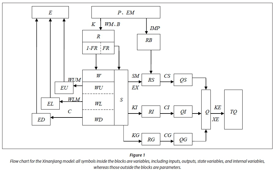
In the Xinanjiang model, the basin is divided into a set of sub-basins. The outflow from each sub-basin is first simulated and then routed down the channels to the main basin outlet. The flow chart is shown in Fig. 1. Based on the concept of runoff formation on repletion of storage, the simulation of outflow from each sub-basin is computed in 4 major steps:
1.Evapotranspiration and runoff production: the evapotranspiration that generates the deficit of the soil storage is divided into 3 layers: upper, lower, and deep; the runoff production that produces the runoff according to the rainfall and soil storage deficit.
2.Separation of runoff components: the runoff separation that divides the previously determined total runoff into 3 components: surface runoff, subsurface runoff, and groundwater runoff.
3.Overland flow concentration within each sub-basin: this is represented by the convolution with an empirical unit hydrograph or by linear reservoir to produce Q, the sub-basin outflow. In this paper, we calculate the surface flow, interflow and groundwater of sub-basin outflow. Respectively, by linear reservoir (parameters CS, CI and CG in Fig. 1).
4.River network flow concentration: flood routing from the sub-basin outlets to the total basin outlet is achieved by applying the Muskingum method to successive sub-reaches (parameters KE and XE in Fig. 1).
The flow chart for the Xinanjiang model is given in Fig. 1. The inputs of the model were rainfall (P) and measured pan evaporation (EM). The outputs were the discharge (TQ) from the whole basin and the actual evapotranspiration (E), which includes 3 components, EU, EL, and ED.
The state variables were the area mean tension water storage (W) and the area mean free water storage (S). The area mean tension water (W) had 3 components (WU, WL, and WD) in the upper, lower, and deep layer. FR is the runoff-contributing area factor that was related to W. The rest of the symbols inside the blocks were all internal variables. RB was the runoff directly from the small portion of impervious area. R was the runoff produced from the pervious area and divided into 3 components (RS, RI, and RG), referred to as surface runoff, subsurface runoff, and groundwater runoff, respectively. The three components were further transferred into QS, QI, and QG, and together form the total inflow to the channel network of the sub-basin. The outflow of the sub-basin was Q. Then, the Muskingum method was used to calculate the discharge (TQ).
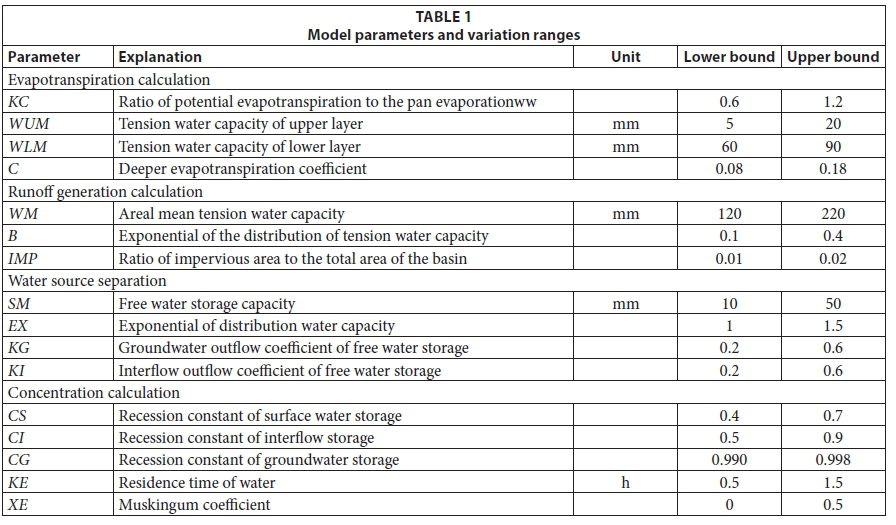
The model had 16 parameters: evapotranspiration parameters K, WUM, WLM and C; runoff production parameters WM, B and IMP; parameters of runoff separation SM, EX, KI and KG; runoff concentration parameters CS, CI and CG; Muskingum parameters KE and XE. The details of the Xinanjiang model and the parameter calibration refer to Qu et al. (2012). There are 14 parameters used in the Xinanjiang model. Additionally, another 2 parameters are used for flow routing along the main rivers (see Table 1 for a list of the 16 model parameters). Generally, the output is more sensitive to 9 parameters (Zhao 1992): KC, SM, KI, KG, CS, CI, CG, KE and XE. For the daily model, there are only 4 sensitive parameters, that is, KC, SM, KI and KG (Song et al., 2013; Zhijia et al., 2011).
Change detection (parameters comparison)
Qu et al. (2012) used 3 different methods to evaluate the land use/cover change effects on hydrological processes in Dapoling basin. In this study, we only compare the best calibrated parameters of different periods to assess the influence of land use change on runoff generation.
Model parameters might be different when the model is calibrated to different time periods. The Xinanjiang model consists of 16 parameters, and 9 of these (KC, SM, KI, KG, CS, CI, CG, KE, XE) (Table 1) are very sensitive to the calibration process (Song et al., 2013; Zhao, 1992; Zhijia et al., 2011). As a result, the calibration process is time consuming. To reduce this complexity, a methodology for system decomposition and degeneration of dimensionality has been developed in the calibration of the Xinanjiang model. By decomposition, the model structure is analysed hierarchically. The calibration is carried out from a lower to higher hierarchy; to this end, different objective functions are used for different levels. The objective of degeneration is to reduce the number of parameters being optimized simultaneously to at least 3 or fewer. The reduction is based on the sensitivity analysis and structure constraint. For example, there is a daily model and an hourly model for the Xinanjiang model. The objective function for the daily model is to keep the mean annual water balance, which means KC is the most important parameter that needs to be calibrated. Those insensitive parameter values (e.g. WUM, WLM, C and so on) can be chosen by experience. In this study, the daily model and linearized parameter calibration method are used for automatic parameter calibration of the Xinanjiang model.
Linearized parameter calibration method
The linearized calibration method is a new optimization algorithm. It was developed to solve the theoretical problem of unrelated local optima produced in the nonlinear model parameter calibration by using the objective function based on error sum of squares. The calibrated parameter values are stable when using different initial parameter values via the linearized calibration method, which can find the true parameter values without producing unrelated local optima. Furthermore, compared with the SCE-UA method and the simplex method, the linearized calibration method has higher calculation accuracy and convergence rate and the parameter calibration results are also very stable, i.e., not influenced by the different initial parameter values. In the real model study, the method can also find the unique global optima and has good performance in parameter calibration. The linearized calibration method is an efficient, effective, and robust calibration method (Bao and Zhao, 2014; Bao et al., 2013). The basic principles and derivation process of the linearized calibration method are as follows:
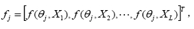
The traditional parameter estimation method is based on the objective function of the minimum-sum-squared error. For any function f:

where: θ is parameter vector, X is independent variable vector. The objective function of minimum-sum-squared error is constructed as:
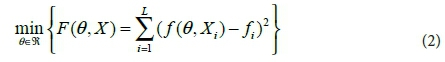
where: 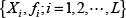 is the sample series for parameter calibration. It can be observed that Eq. 2 increases the power of linear parameter from 1 to 2 and for a linear function this is clearly correct. However, the sum-squared causes the increase in unrelated optimal values when solving nonlinear function parameter optimization problems. For example, if the power of parameters is equal to or greater than 2, sum-squared will double the power of parameters, which will be reduced only by 1 through first-order derivation - thus, it will increase the number of parameter solutions. A 1-parameter function with 1 sample is employed to demonstrate the problem. It can be seen from the analysis that the objective function of the minimum-sum-squared error works well in parameter optimization for a linear function; however, this is not the case for a nonlinear function.
Based on this analysis, we developed a linearized parameter calibration method. Firstly, we linearize the nonlinear function using parameters as independent variables. Secondly, the linearized parameters can be calibrated with the objective function of minimum-sum-squared error. Finally, iteration is adopted to gradually approach the optimal value of nonlinear function parameters.
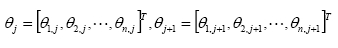
The forward difference of the partial derivative of f as in Eq. 1 with respect to parameter θi:
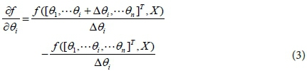
In the calibration process, θi,j represents estimation of θi in Step j and θi,j+1 is j+1 step estimation of θi. Substituting θi,j and θi,j+1into Eq. 3, we obtain:
Eq. 4 can be rewritten as:
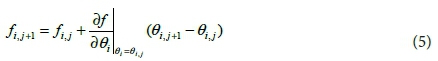
Eq. 5 shows the relation of the parameters, function values and partial derivation with respect to parameters in the adjacent 2 steps in the parameter searching process. The partial derivation with respect to a parameter exhibits the degree of function variation resulting from the variation of parameters. Usually, the greater the degree of function change, the more sensitive the parameter is in the function, which is called parameter sensitivity. Considering the variation of all parameters in the consecutive 2 steps, Eq. 5 can be transformed into:
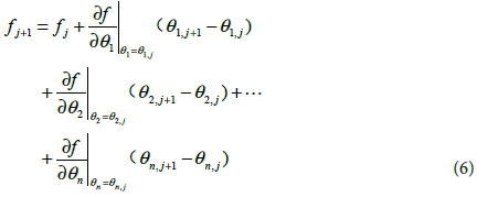
Eq. 6 is the linear approximate of nonlinear function f with respect to parameter θ. In the process of parameter calibration, we assume L groups of observation samples:

Substitute it into Eq. 6:
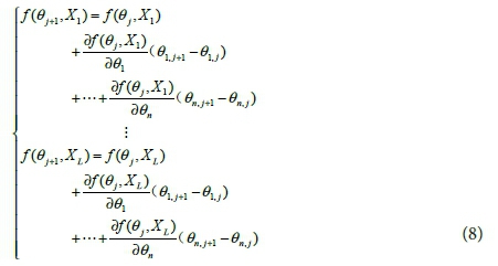
The vector matrix of Eq. 8 is:

where:
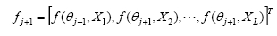
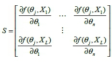
is called parameter sensitivity matrix. Eq. 9 is the linear approximation of actual function f. Substitute the observation sample into Eq. 9 and it can be written as:

where 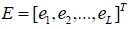 is the difference between f and fj+1. As the iterative process continues, the difference between f and fj+1 approaches a minimum. We obtain:

where  is observation vector. The optimal estimation value of θj+1 can be inferred from Eq. 10 in the linear condition:

Considering Eq. 9 is the linear approximation of actual function f(θ, X), which cannot guarantee that θj+1 is the optimum in the searching direction, a scale coefficient b needs to be multiplied to make the actual error function the optimum in the searching direction.

The variation range of b is (0, 1), which can be determined by minimum-sum-squared error of actual function:

Eq. 12 determines the searching direction, and Eqs 13 and 14 determine the step length of parameter, which not only ensures the correct searching direction, but also satisfies the minimum error in the searching direction. Eqs 12, 13 and 14 comprise the linearized parameter calibration method, which has a similar form to the Gauss-Newton iteration method, but a different theoretical basis.
Since the linearized parameter calibration method uses linear approximation of Eq. 9 as a function, the construction of the objective function of sum-squared error and the first-order derivation of objective function to search the optimum will not add unrelated local optima. It is proved that the linearized parameter calibration method can ensure the correctness of every step in searching direction.
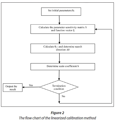
Considering the error resulting from Eq. 10, the searching process of linearized parameter calibration method is the process of step-by-step approach to the optimum. Its procedure is as follows:
1.Set an initial value of parameter θ0
2.Calculate the parameter sensitivity matrix S and function vector fj according to the parameter vector
3.Determine new parameter vector θj+1 and search direction ∆θ = θj+1 −θj with Eq. 12
4.Determine scale coefficient b with Eq. 14
5.The search will be stopped if θj+1 arrives at the optimum individual. If not, return to Step (2) and go on to the next iterative operation. The framework flow chart for the linearized parameter calibration method is shown in Fig. 2.
It can be seen that the linearized parameter calibration method is simpler than the conventional optimization method from Step (3) of the calculation process. The optimal parameter vector θj+1 can be determined through θj and linear condition using Eq. 12 instead of the trial-and-error method.
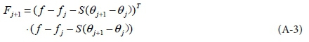
To prove the validity of Step (3) that ensures the correct searching direction ∆θ=θj+1-θj, we only need to verify the error Fj+1 corresponding to new parameter vector θj+1 of any step calculated by Eq. 12 is less than Fj corresponding to the above step parameter vector θj. The proof is shown in Appendix 1.
APPLICATION EXAMPLE
Ideal model verification
Nonlinear function parameter calibration refers to nonlinear parameter calibration of explicit function, which can obtain derivation with respect to parameters directly. The following general nonlinear parameter function is used in this paper:

Here, this function is adopted as the nonlinear parameter function, because there is only one independent variable x in this function and 2 parameters θ1, θ2. In addition, these 2 parameters for the independent variables are highly nonlinear, and the function is relatively simple in the expression, but the function structure (due to the relationship between variables and parameters) is complex. The superiority of the parameter calibration method can be explained more clearly by using this function.
The derivation function of a parameter is:
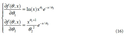
Ideal model refers to the model with no error in the independent variable, dependent variable and parameters. We assume θ1 = 2 and θ2 = 10 in the ideal model, as Eq. 15 and x varies in the range of [1, 100] with equal intervals.
Table 2 lists the process of searching parameters in every step, starting from a group of initial parameters (θ1,0 = 1.2427; θ2,0 = 49.4716). It can be seen from Table 2 that the parameters sought from every step follow a loop approach; the true value and the objective function of sum-squared error gradually decrease in the process of searching, as does the searching step length in every loop. In the beginning, sum-squared error and searching step length are large and they decrease sharply after several iterations, which demonstrates the significant convergence and effectiveness of the linearized parameter calibration method.

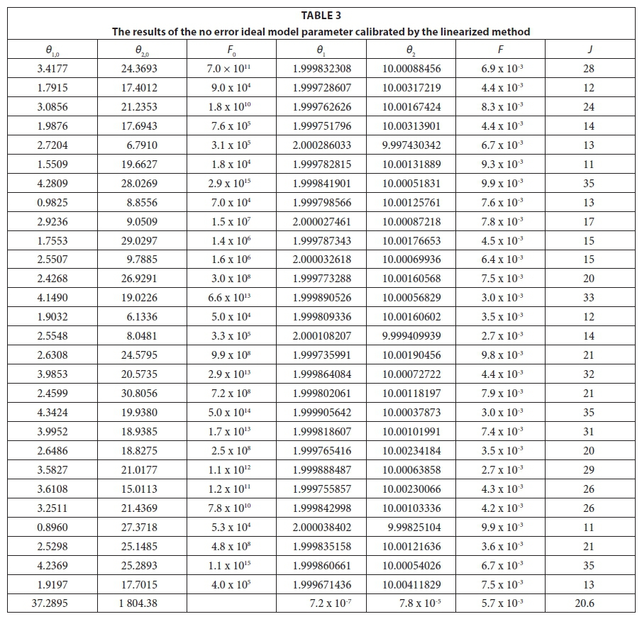
Table 3, on the next page, summarizes the calibration results starting from different initial parameter values. In the table, J is an iterative step for searching for optimum.
According to the results given in Table 3:
1.The influence of initial parameter value is minor for linearized parameter calibration. The square deviation of a parameter decreased from the initial value of 37.2895 and 1 804.38 to the final optima of 7.2 × 10⁻⁷ and 7.8 × 10⁻⁵, respectively.
2.The linearized parameter calibration method is objective with a high degree of accuracy. The relative error between the results and true value of every trial are 9.5 × 10⁻⁵ and 16.3 × 10⁻⁵.
3.The iteration number of the linearized parameter calibration is low, and the effect is good. According to the results from Table 3, the minimum iteration number is 11, the maximum number is 35 and the average loop number is 20.6.
Table 4 demonstrates the calibration results with consideration of error in the dependent variable. The error was generated using a normal distribution model. The error proportion is the average per cent relative to the true value of the function f(θ; x). D is the distance between the evaluated parameter and the true value, calculated by Eq. 17:

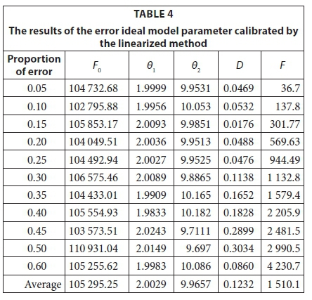
According to the results from Table 4, the error of dependent variable has certain but little influence on the parameter estimation. The average of relative error distance is only 1.21%.
Case study
Dapoling Station was used as a case study application, situated in the upper reaches of Xixian basin with a drainage basin of 1 640 km2; the length of its main channel is 73 km (Fig. 3).
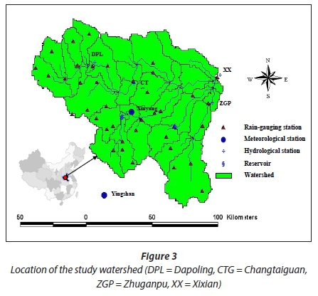
The river flows through mountainous terrain with many tributaries and a steep slope; runoff is intermittent and vulnerable to zero flow in the dry season. There are not many water conservancy projects in the basin and rice is the dominant crop grown there, followed by wheat.
Xixian basin is situated in the transition zone between the northern subtropical region and the warm temperate zone. Rainfall for the flood season is mainly affected by monsoon; and the long-term mean annual precipitation is 1 145 mm (calculated by the data from 1954 to 2000). Half of the precipitation (~50%) falls between June and September. For further details of the watershed refer to Qu et al. (2012).
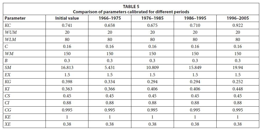
The Dapoling basin is serviced by 13 precipitation stages and one discharge stage (Dapoling stage). There is no evaporation stage in this catchment; because of this, the Nanwanevaporation stage data were used for the evaporation calculation. Series of observed data included daily precipitation of 13 rainfall stages, daily evaporation of Nanwan stage and daily discharge of Dapoling stage from 1966 to 2005. The total series were divided into 10-year periods for parameter calibration, 4 periods in all; that is, from 1966-1975, 1976-1985, 1986-1995 and 1996 to 2005. The initial parameter values are presented in Table 5.
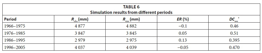
Also, Table 5 shows the results of parameter calibration in different periods. Table 6 lists the performance of the calibrated parameters. From Table 6, the calibrated parameters using the linearized parameter calibration method can give good simulation results: relative errors of 4 different periods from 1964 to 2005 are −0.1%, 0.05%, 0.13% and −0.05%, respectively. The greatest relative error is 0.13% and all errors are less than 0.15%, which means that the proposed method is reliable in terms of water budgets. From Table 5, it can be seen that the change of the ratio of potential evapotranspiration to pan evaporation, KC, is highly significant, increasing from 0.658 to 0.922. A higher ratio means higher evapotranspiration from the basin, which causes a decrease in runoff. Additionally, the increase in free water storage capacity, SM, reflects the decrease in surface runoff. Although the sum of the outflow coefficient KG (free water storage to the groundwater flow) and KI (free water storage to the interflow) is kept constant, the single value of each parameter has changed. KI changed towards a larger proportion (increase of interflow), while KG decreased from 0.334 to 0.252 (Table 5), causing higher peak flows and a quicker recession.
CONCLUSIONS
Streamflow at the outlet is the comprehensive response of the whole basin system to the input, precipitation, and thus, invariably, to the change of underlying surface in the basin. In appreciation of this fact, a number of studies have focused on using conceptual rainfall-runoff models to quantify the effect of land use and land cover change on runoff dynamics. However, because of the large number of parameters in the hydrological model, an effective automatic calibration method becomes important. Thus, a linearized parameter calibration method is presented for solving this problem. Unlike the previous study by Qu et al. (2012), we only use parameter comparison to assess the influence of land use/cover change on runoff of the basin. Compared to the method based on the error square sum, the linearized parameter calibration method has the following advantages:
• It can solve the theoretical problem of added unrelated local optimums
• The convergence of the method can be strictly proven in theory
• The determination of seeking direction and step length is objective and effective
In addition, this method was applied for parameter calibration of the Xinanjiang model in the upper Huaihe River Basin to evaluate the effect of land use change on hydrological processes through the change of parameters, for example, KC, SM, KI and KG. An increase in KC means higher evapotranspiration in the upper Huaihe River Basin, which causes a decrease in runoff. An increase in SM means a decrease in surface runoff. The increase in KI and decrease in KG in Dapoling basin reveal that the present land use pattern causes high peak flows and quicker recession. Because of limited data availability, only the daily model was applied for parameter calibration and evaporation, and runoff generation parameters were compared, while water source separation and concentration parameters were not.
The linearized parameter calibration method is a new calibration method. Future studies will involve tested the method in more basins and using more hydrological model parameter calibrations.
ACKNOWLEDGEMENTS
This study is supported by National Natural Science Foundation of China (No. 41371048/51479062/51279057), Nonprofit Special Research Project of Ministry of Water Resources of China (Grant Nos. 201401034).
REFERENCES
BARDOSSY A and SINGH S (2008) Robust estimation of hydrological model parameters. Hydrol. Earth Syst. Sci. 12 (6) 1273-1283. https://doi.org/10.5194/hess-12-1273-2008 [ Links ]
BAO W (1991) Model parameter estimation with colored noise. J. Hydraul. Eng. 12 47-52. [ Links ]
BAO W and ZHAO L (2014) Application of linearized calibration method for vertically mixed runoff model parameters. J. Hydrol. Eng. 19 (8) 04014007. https://doi.org/10.1061/(asce)he.1943-5584.0000984 [ Links ]
BAO W, LIN Y, HUANG X, QU S and ZHAO C (2004) Parameter robust estimation of reach flood concentration model. J. Wuhan Univ. Hydraul. Elec. Eng. 37 (6) 3-17. [ Links ]
BAO WM, WEI SI and SI-MIN QU (2013) The linearized calibration method of non-linear function parameter. Chin. J. Comput. Mech. 30 (2) 236-241. [ Links ]
BURNS D, VITVAR T, MCDONNELL J, HASSETT J, DUNCAN J and KENDALL C (2005) Effects of suburban development on runoff generation in the Croton River basin, New York, USA. J. Hydrol. 311 (1) 266-281. https://doi.org/10.1016/j.jhydrol.2005.01.022 [ Links ]
CHAU KW (2007) An ontology-based knowledge management system for flow and water quality modeling. Adv. Eng. Softw. 38 (3) 172-181. https://doi.org/10.1016/j.advengsoft.2006.07.003 [ Links ]
CHEN W and CHAU KW (2006) Intelligent manipulation and calibration of parameters for hydrological models. Int. J. Environ. Pollut. 28 (4-Mar) 432-447. https://doi.org/10.1504/IJEP.2006.011221 [ Links ]
CHENG C, CHAU K, SUN Y and LIN J (2005) Long-term Prediction of Discharges in Manwan Reservoir using Artificial Neural Network Models. Lecture Notes Comput. Sci. 3498 (12) 1040-1045. https://doi.org/10.1007/11427469_165 [ Links ]
CHENG C-T, OU C and CHAU K (2002) Combining a fuzzy optimal model with a genetic algorithm to solve multi-objective rainfall-runoff model calibration. J. Hydrol. 268 (1) 72-86. https://doi.org/10.1016/S0022-1694(02)00122-1 [ Links ]
CHENG C-T, WANG W-C, XU D-M and CHAU K (2008) Optimizing hydropower reservoir operation using hybrid genetic algorithm and chaos. Water Resour. Manage. 22 (7) 895-909. https://doi.org/10.1007/s11269-007-9200-1 [ Links ]
DUAN Q, SOROOSHIAN S and GUPTA V (1992) Effective and efficient globaloptimization for conceptual rainfall‐runoff models. Water Resour. Res. 28 (4) 1015-1031. https://doi.org/10.1029/91WR02985 [ Links ]
FRANCHINI M (1996) Use of a genetic algorithm combined with a local search method for theautomatic calibration of conceptual rainfall-runoff models. Hydrol. Sci. J. 41 (1) 21-39. https://doi.org/10.1080/02626669609491476 [ Links ]
FRANCHINI M and GALEATI G (1997) Comparing several genetic algorithm schemes for the calibration of conceptual rainfall-runoff models. Hydrol. Sci. J. 42 (3) 357-379. https://doi.org/10.1080/02626669709492034 [ Links ]
GUO WJ, WANG CH, MA TF, ZENG XM and YANG H (2016) A distributed Grid-Xinanjiang model with integration of subgrid variability of soil storage capacity. Water Sci. Eng. 9 (2) 97-105. https://doi.org/10.1016/j.wse.2016.06.003 [ Links ]
GUPTA H, SOROOSHIAN S and DUAN Q (1998) Calibration of rainfall-run models: Application of the global optimization to the sacramento soil moisture accounting model. Water Resour. Res. 34 (4) 1015-1030. https://doi.org/10.1029/97WR03495 [ Links ]
GUPTA HV, SOROOSHIAN S and YAPO PO (1998) Toward improved calibration of hydrologic models: Multiple and noncommensurable measures of information. Water Resour. Res. 34 (4) 751-763. [ Links ]
HENDRICKSON JD, SOROOSHIAN S and BRAZIL LE (1988) Comparison of Newton-type and direct search algorithms for calibration of conceptual rainfall-runoff models. Water Resour. Res. 24 (5) 691-700. https://doi.org/10.1029/WR024i005p00691 [ Links ]
JIANG H, REN L, AN R, YUAN F and WANG M (2004) Application of remote sensing information about land use and land cover to flood simulation. J. Hohai Univ. (Nat. Sci.) 32 131-135. [ Links ]
JOHNSTON P and PILGRIM D (1976) Parameter optimization for watershed models. Water Resour. Res. 12 (3) 477-486. https://doi.org/10.1029/WR012i003p00477 [ Links ]
JU Q, YU Z, HAO Z, OU G, ZHAO J and LIU D (2009) Division-based rainfall-runoff simulations with BP neural networks and Xinanjiang model. Neurocomputing 72 (13) 2873-2883. https://doi.org/10.1016/j.neucom.2008.12.032 [ Links ]
MUTTIL N and CHAU KW (2006) Neural network and genetic programming for modelling coastal algal blooms. Int. J. Environ. Pollut. 28 223-238. https://doi.org/10.1504/IJEP.2006.011208 [ Links ]
QU S, BAO W, SHI P, YU Z, LI P, ZHANG B and JIANG P (2012) Evaluation of runoff responses to land use changes and land cover changes in the Upper Huaihe River Basin, China. J. Hydrol. Eng. 17 (7) 800-806. https://doi.org/10.1061/(ASCE)HE.1943-5584.0000397 [ Links ]
RITZEL BJ, EHEART JW and RANJITHAN S (1994) Using genetic algorithms to solve a multiple objective groundwater pollution containment problem. Water Resour. Res. 30 (5) 1589-1603. https://doi.org/10.1029/93WR03511 [ Links ]
RUSLI SR, YUDIANTO D and LIU JT (2015) Effects of temporal variability on HBV model calibration. Water Sci. Eng. 8 (4) 291-300. https://doi.org/10.1016/j.wse.2015.12.002 [ Links ]
SAVIC DA, WALTERS GA and DAVIDSON JW (1999) A genetic programming approach to rainfall-runoff modelling. Water Resour. Manage. 13 (3) 219-231. https://doi.org/10.1023/A:1008132509589 [ Links ]
SONG X, KONG F, ZHAN C, HAN J, ZHANG X and YU Y (2013) Parameter identification and global sensitivity analysis of Xin'anjiang model using meta-modeling approach. Water Sci. Eng. 6 (1) 1-17. [ Links ]
TAO XE, CHEN H, XU CY, HOU YK and JIE MX (2015) Analysis and prediction of reference evapotranspiration with climate change in Xiangjiang River Basin, China. Water Sci. Eng. 8 (4) 273-281. https://doi.org/10.1016/j.wse.2015.11.002 [ Links ]
TAORMINA R, CHAU K-W and SETHI R (2012) Artificial neural network simulation of hourly groundwater levels in a coastal aquifer system of the Venice lagoon. Eng. Appl. Artif. Intell. 25 (8) 1670-1676. https://doi.org/10.1016/j.engappai.2012.02.009 [ Links ]
VASQUEZ JA, MAIER HR, LENCE BJ, TOLSON BA and FOSCHI RO (2000) Achieving water quality system reliability using genetic algorithms. J. Environ. Eng. 126 (10)954-962. https://doi.org/10.1061/(ASCE)0733-9372(2000)126:10(954) [ Links ]
WAN R and YANG G (2004) Progress in the hydrological impact and flood response of watershed land use and land cover change. J. Lake Sci. 16 (3) 258-264. https://doi.org/10.18307/2004.0311 [ Links ]
WANG G, LIU J, KUBOTA J and CHEN L (2007) Effects of land-use changes on hydrological processes in the middle basin of the Heihe River, northwest China. Hydrol. Process. 21 (10) 1370-1382. https://doi.org/10.1002/hyp.6308 [ Links ]
WANG Q (1991) The genetic algorithm and its application to calibrating conceptual rainfall-runoff models. Water Resour. Res. 27 (9) 2467-2471. https://doi.org/10.1029/91WR01305 [ Links ]
WANG W-C, CHAU K-W, CHENG C-T and QIU L (2009) A comparison of performanceof several artificial intelligence methods for forecasting monthly discharge time series. J. Hydrol. 374 (3) 294-306. https://doi.org/10.1016/j.jhydrol.2009.06.019 [ Links ]
WU CL, CHAU KW and LI YS (2009) Predicting monthly streamflow using data-driven models coupled with data-preprocessing techniques. Water Resour. Res. 45 (8) 2263-2289. https://doi.org/10.1029/2007WR006737 [ Links ]
YAO C, LI Z, YU Z and ZHANG K (2012) A priori parameter estimates for a distributed, grid-based Xinanjiang model using geographically based information. J. Hydrol. 468 47-62. https://doi.org/10.1016/j.jhydrol.2012.08.025 [ Links ]
YAPO PO, GUPTA HV and SOROOSHIAN S (1996) Automatic calibration of conceptual rainfall-runoff models: sensitivity to calibration data. J. Hydrol. 181 (1) 23-48. https://doi.org/10.1016/0022-1694(95)02918-4 [ Links ]
YUAN Y and SHI P (2001) Effect of land use on the rainfall runoff relationship in a basin-SCS modelapplied in Shenzhen city. J. Beijing Normal Univ. (Nat. Sci.) 37 131-136. [ Links ] .
ZÁDOR J, ZSÉLY LG & TURÁNYI T (2006) LOCAL and global uncertainty analysis of complex chemical kinetic systems. Reliab. Eng. Syst. Saf. 91 (10) 1232-1240. https://doi.org/10.1016/j.ress.2005.11.020 [ Links ]
ZHANG L, LI X, WANG Z and LI X (2004) Study and Application of SWAT Model inthe Yunzhou Reservoir Basin. J. China Hydrol. 24 (3) 4-8. https://doi.org/10.1016/j.wse.2016.07.001 [ Links ]
ZHANG ST, LIU Y, LI MM and LIANG B (2016) Distributed hydrological models for addressing effects of spatial variability of roughness on overland flow. Water Sci. Eng. 9 (9) 249-255. [ Links ]
ZHAO R (1992) The Xinanjiang model applied in China. J. Hydrol. 135 (1) 371-381. [ Links ]
ZHIJIA L, PENGLEI X and JIAHUI T (2013) Study of the Xinanjiang model parameter calibration. J. Hydrol. Eng. 18 1513-1521. https://doi.org/10.1061/(ASCE)HE.1943-5584.0000527 [ Links ]
ZHONG-BO YU, YANG T and SCHWARTZ FW (2014) Water issues and prospects for hydrological science in China. Water Sci. Eng. 7 (1) 1-4. [ Links ]
Received 24 September 2015
Accepted in revised form 16 March 2017
* To whom all correspondence should be addressed. e-mail: lindongsisi@163.com or wanily@hhu.edu.cn
The validity of parameter search is justified as follow. From the text we can get the sum of squared errors Fj corresponding to the above step parameter vector θj.

The sum of squared errors Fj+1 can be expressed as:

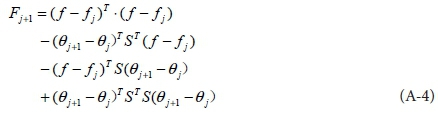
Substitute Eq. 9 into Eq. A-2:
then:
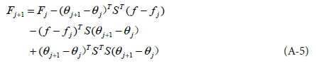
Substitute Eq. 12 into Eq. A-5:
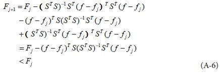
It can be observed that the new parameter vector θj+1 of any step determined by Eq. 12 satisfying the relation:

According to Eq. A-7, every searching step will get less sum-squared. As the iterative process continues, the sum-squared error approaches the minimum value and the optimal parameter will be obtained. So the searching direction determined by Eq. 12 is correct.

